Analysis of the Energy Efficiency Improvement in a Load-Sensing Hydraulic System Built on the ISO Plate

Abstract

The article presents a proposal to reduce energy consumption in a hydraulic system with a single pump and multiple receivers. The proposed Load-Sensing Basic (LSB) solution consists of expanding a typical hydraulic system by using additional logic valves and a dedicated differential valve. The modification is aimed at decrease in operating pressure and, thus, reduction in energy consumption. The LSB system is compact as all components are built on a single ISO plate. A detailed mathematical model of the system was formulated, then a simulation model was built and numerical tests were carried out in the Matlab/Simulink environment. The obtained results indicate that the use of the proposed LSB system for the implementation of typical working cycles with three actuators may reduce energy consumption by 4–30%, and under certain conditions even up to 70%.

1. Introduction

Heavy-duty machines and working equipment often use hydraulic drives consisting of a single fixed-delivery pump which supplies multiple receivers. This solution is economically viable, as the system is relatively simple and constructed of typical low-cost components. Hence, it is commonly used in heavy duty machines and industrial systems. In the case when the pump’s delivery is higher than the total demand of all receivers, the excessive flow is discharged through the relief valve to the tank. Appropriate control of the hydraulic elements makes it possible to obtain even complex working movements of receivers, thus automating the operation process. In particular, solenoid-operated proportional valves offer great possibilities for fast and precise control. The main disadvantage of throttling systems supplied with a single pump of a constant capacity, when the pump’s output is not fully utilized, is significant energy loss. The loss results from the fact that the excessive fluid flow rate is drained back to the tank at the pressure set on the relief valve. This wasted energy is converted into heat, which in turn may require the use of additional oil coolers.

The issue of reducing energy losses in hydraulic systems is taken up in scientific works. The research covers various solutions, including structural modifications to the pump, the use of control valves, a converter or a compensator, the storage of excess energy with accumulators, etc. A load-sensing design for a pump in the electro-hydraulic actuator system (EHA) was designed by Chao et al. [1] in order to reduce energy waste. The solution consisted in the use of a specially designed spool valve in order to decrease the volumetric displacement of the pump automatically as the load pressure increases. As a result, the motor torque and heat generation are reduced. Shang et al. [2] proposed a novel integrated Load-Sensing Valve-Controlled Actuator (LSVCA) with high efficiency and low energy consumption, which can reduce the overflow loss by the intermittent operation of the motor and reduce the throttling loss by the variation of the supply pressure. Numerical and experimental studies showed the 1.75-fold throttling efficiency improvement. Analysis of a directional control valve for load-sensing application using CFD numerical modelling was carried out by Bigliardi et al. [3]. Discharge coefficient, efflux angle, flow forces, pressure and velocity distributions in the critical region were estimated based on the simulation results. A wide research on energy saving by means of improvement hydraulic system efficiency was carried out by Gradl and Scheidl. As a result, a hydraulic stepper converter consisting of a hydraulic cylinder piston unit and a fast-switching valve was developed [4] and oscillating mass converter (OMC) with a pure hydraulic control [5] was proposed. Similarly, fast-switching valves were used by Pan et al. [6] in a novel approach for increasing energy efficiency in the fluid power systems, that resulted in an approximately one-seventh reduction in power loss compared to a conventional system based on throttle valves. Another proposal of an energy saving strategy for an electrohydraulic servo valve system was proposed by W. Wang and B. Wang [7]. The strategy, based on the use of load-sensing pump, proportional relief valve together with adaptive backstepping sliding mode control, allowed energy savings of 62% in harmonic tests and up to 90% in multi-step tests. In the field of research on hydraulic systems of heavy-duty machines, solutions for improving the energy efficiency of excavators or manipulators are often presented. Bedotti et al. described several different methods to reduce losses, improve fuel-saving and energy recovery [8] as well as presented energy comparison of system layouts for a hydraulic excavator [9]. The results obtained led to the development of a new hybrid excavator concept with a 15% reduction in fuel consumption. Moreover, minimizing the energy demand of a heavy-load mobile manipulator using a novel electro-hydraulic drive system was the subject of research by Ding et al. [10], while Cheng et al. [11] developed a load-sensing system for an excavator based on two switching valves for controlling flow and pressure separately. A proposal to further improve the efficiency of a typical load-sensing system by reducing inherent pressure losses (SIPL) was formulated by Siebert et al. [12]. The carried out simulations showed that pressure loss may be reduced by up to 44%.

Research on these types of systems is usually carried out with the use of numerical simulation. The principles and methods of hydraulic equipment modelling were summarized in the book by Novak et al. [13]. This methodology was then successfully applied in a number of studies, including research on an adjustable flow control valve by Kuehnlein et al. [14], electro-hydraulic proportional valve by Rybarczyk et al. [15], excavator hydraulic system by Casoli et al. [16] or proportional flow control valve by Lisowski et al. [17]. Moreover, Naseradinmousavi and Nataraj [18] described a non-linear modelling method of solenoid-driven butterfly valves, while Du and Nydal [19] formulated numerical schemes for transient flow in one dimension. A comparison of various numerical modelling approaches related to water hydraulic systems was presented by Antelmi et al. in [20].

This article proposes a method of reducing energy consumption in a Load-Sensing Basic (LSB) system, adapted for installation on a standard ISO 4401 plate. Typical components designed for mounting on the plate were used, including proportional and logic valves and a differential valve. The introduction of an additional differential valve resulted in a pressure drop and hence some energy loss. However, taking into account the global energy demand of the system, it has been significantly reduced in typical practical applications. Using the Matlab/Simulink environment, model of the LSB system with three actuators was built. The carried out simulation tests took into account the implementation of different work cycles by actuators under various loads. The energy demands for the base system and the LSB system were determined and compared.

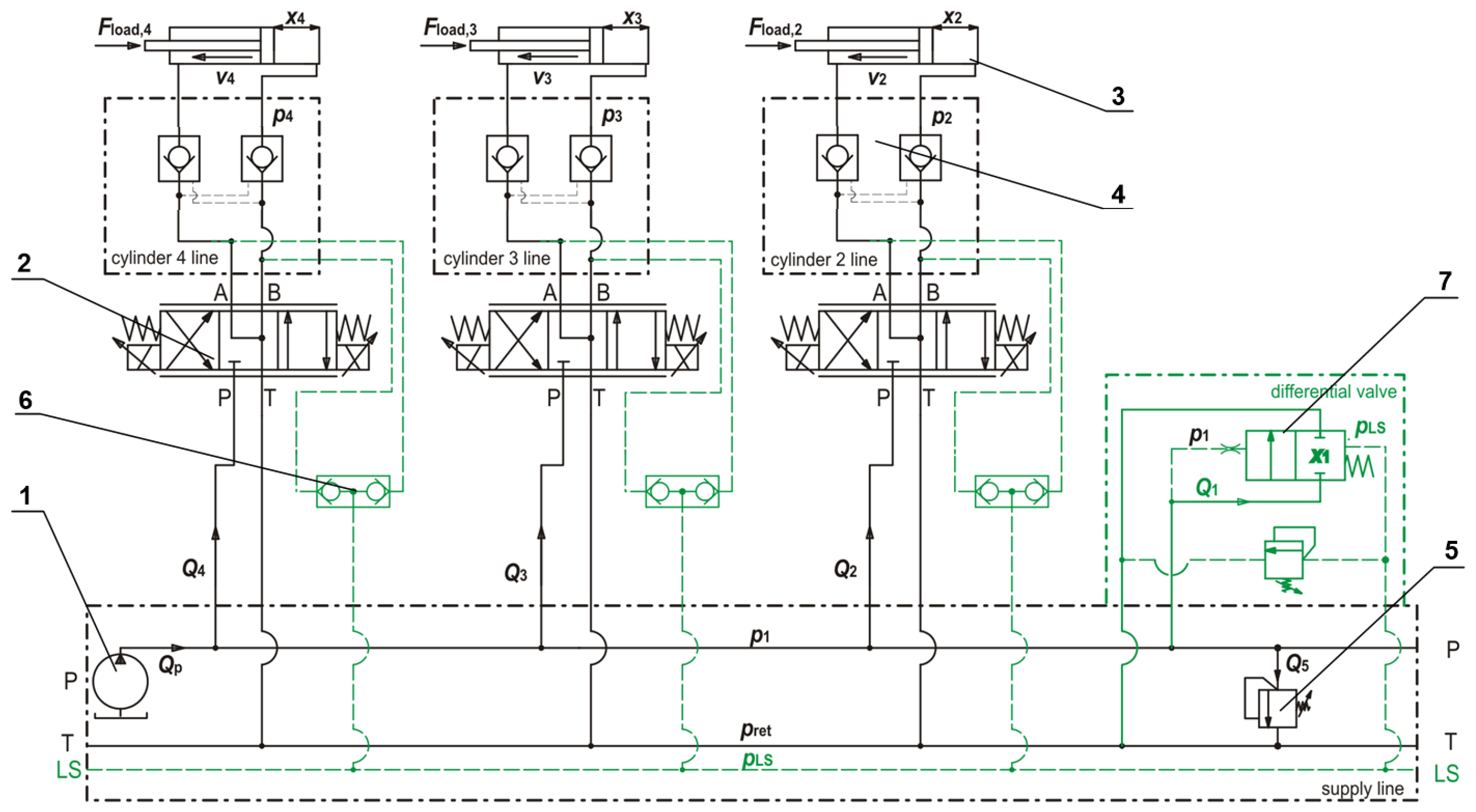
2. Working Principle of the Analysed System

The subject of the analysis is a hydraulic system which is shown in Figure 1. The valve block has been mounted on a standard ISO 4401 plate with a nominal size of DN 6. There are three lines with hydraulic actuators in the system. The lines are powered from a fixed delivery pump (1) of nominal flow rate $Q_{nom}=80$ dm³ min⁻¹, with maximum outputs to the receivers $Q_{max,i}=40$ dm³ min⁻¹ at a maximum pressure of $p_{max}=32$ MPa. Relief valve (5) provides protection against overpressure. The flow to individual receivers (3) is controlled by means of three proportional valves (2), and the tightness is ensured by hydraulic locks (4). The presented system is simple, reliable in operation and hence often used in practice. However, in the event that not all actuators are running simultaneously or the total flow requirement of the actuators is less than the pump delivery, significant energy losses may occur in the system. The loss is related to keeping the high supply line pressure, which is only limited by the operation of the relief valve.

In order to reduce energy losses, it was proposed to modify the system by adding the LSB module, which is shown in green in Figure 1. For economic and practical reasons, the same ISO connection plate and control valves with hydraulic locks were used in the extended system. The LSB module contains three sets of logic valves (6) which receive load signals from individual actuator lines and a differential valve (7) to decrease supply line pressure. All the included elements are typical hydraulic components with known flow characteristics and connection dimensions. This ensures low costs and short expansion time. The LSB control signals are taken directly from the outputs of the proportional control valves in the proposed system. Plate mounted control valves were used in accordance with ISO 4401-03-03 which, in the neutral position, provide an open connection between the actuator lines and the return line. Thus, when all control valves are in neutral position, no pressure appears on the LSB line, so the differential valve opens and the supply line is discharged. Similarly, when the total flow requirement of all actuators is lower than the pump output, and the pressure in the line of the most loaded actuator is lower than that set on the relief valve (5), the required power supplied to the pump is reduced compared to the classic system without LSB. This study uses the results of previous work on flow calculations and determining the characteristics of proportional distributors, e.g., [21,22]. For the special needs of this system, however, a dedicated differential valve adapted to be mounted on an ISO plate with an integrated safety relief valve was developed.

A key element for the correct operation of the LSB system is the differential valve. The view of the created 3D model of the valve is shown in Figure 2, while the cross-section by a plane passing through the spool axis is presented in Figure 3. The flow through the differential valve takes place between the P and T ports. In the considered design, the A and B ports are not used and both should be plugged. However, in industrial applications there is a possibility to mount, for example, one of the control valves directly on top of the differential valve, since all the channels are pass-through.

The valve consists of a body (1) in which a spool (2) is placed. The stability of the valve operation is achieved by means of a damping nozzle (4) and a spring (3). All connection ports are pass-through, which enables the potential installation of other valves in the sandwich system. The position of the spool $x_1$ is determined by the $F_{p1}$ and $F_{pLS}$ forces resulting from the $p_1$ and $p_{LS}$ pressures, respectively, the $F_t$ viscous friction force, the $F_{h}d$ flow force and the $F_s$ spring force. In the case when $F_{p1}$ value exceeds the sum of $F_{pLS}$ and $F_s$, the $Q_1$ flow is opened and thus the supply line is discharged.

3. Formulating a Mathematical Model

Mathematical model of the studied system was built in accordance with the methodology of modelling hydraulic components, which was introduced by Novak et al. [13]. The created mathematical model consists of a system of differential equations and algebraic formulas. It includes the pump flow rate function, equations of fluid mass conservation formulated for the distinguished volumes, equations of motion of valve spools and hydraulic cylinder pistons, flow equations through throttle gaps based on Bernoulli’s law and geometrical relations. The pump was modelled as an ideal source of flow rate. The flow rate $Q_p$ is assumed to be constant at $Q_{nom}=80$ dm³ min⁻¹ except for a short start-up time $t_s$ when it rises linearly from 0:

$$Q_p\left(t\right)=\left\{\begin{array}{cc}{Q}_{nom}·\frac{t_s}{t}\hfill & \mathrm{for}{t}_s<t\hfill \\ Q_{nom}\hfill & \mathrm{otherwise}\hfill \end{array}\right.$$

(1)

The mass conservation equation formulated for the supply line has the following form:

$$\frac{d{p}_1\left(t\right)}{dt}=\frac{B_f}{V_1}·(Q_p\left(t\right)-Q_1\left(t\right)-Q_2\left(t\right)-Q_3\left(t\right)-Q_4\left(t\right)-Q_5\left(t\right)),$$

(2)

where $Q_1$ refers to the differential valve, $Q_5$ to the relief valve, and $Q_2,Q_3,Q_4$ to the lines of actuators, respectively. The supply line volume $V_1$ and the fluid bulk modulus $B_f$ were assumed to be constant. Analogous equations have been formulated for three lines of actuators based on the flow rates of control valves $Q_i$ as well as positions $x_i$ and velocities $v_i$ of the actuator pistons:

$$\frac{d{p}_i\left(t\right)}{dt}=\frac{B_f}{V_{0,i}+x_i\left(t\right)·A_{C,i}}·(Q_i\left(t\right)-\frac{d{x}_i\left(t\right)}{dt}·A_{C,i}),\mathrm{where}i=\{2,3,4\},$$

(3)

where the output flow rates of three control valves $Q_i$ were calculated on the basis of characteristics obtained within the previous research (Figure 21 in [22]). The flow rates were determined based on the current pressure drop $\mathsf{\Delta }{p}_i=p_1-p_i$ and the percentage value of the control signal $I_i$:

$$Q_i=f(\mathsf{\Delta }{p}_i,I_i),\mathrm{where}i=\{2,3,4\}.$$

(4)

The $p_i$ pressures generate hydrostatic forces acting on the pistons of hydraulic cylinders. The equations take into account the hydrostatic forces acting on both sides of the piston, the viscous friction force and the load force. The following equations of motion were formulated for the pistons:

$$m_{p,i}·\frac{d^2{x}_i\left(t\right)}{d{t}^2}=p_i\left(t\right)·A_{C,i}-p_{ret}·A_{R,i}-{\phi }_i·\frac{d{x}_i\left(t\right)}{dt}-F_{load,i},\mathrm{where}i=\{2,3,4\}.$$

(5)

Protection against overpressure is provided by a relief valve $RV5$. The valve ensures that the pressure is limited to $p_{1,max}=30$ MPa. Flow rate through the relief valve gap of the $A_5$ area is described by the following equation:

$$Q_5\left(t\right)={\mu }_5·A_{g,5}\left(x_5\right)·\sqrt{\frac{2·(p_1-p_{ret})}{\rho }}.$$

(6)

where the poppet position $x_5$ can be determined from the equation of motion:

$$m_5·\frac{d^2{x}_5\left(t\right)}{d{t}^2}=(p_1\left(t\right)-p_{ret})·A_5-{\phi }_5·\frac{d{x}_5\left(t\right)}{dt}-C_5·(x_5\left(t\right)+x_{5,start}).$$

(7)

The proposed solution for reducing energy consumption required the installation of a logic valve system that ensured the determination of the maximum pressure occurring in the actuator lines. The pressure signal $p_{LS}$ is the maximum value of all actuator lines which, however, is limited to the relief valve pressure $p_{1,max}$:

$$p_{LS}\left(t\right)=MIN(MAX(p_2,p_3,p_4),p_{1,max}).$$

(8)

The obtained $p_{LS}$ signal is directed to the differential valve. Flow through the valve depends on the pressure difference acting on both sides of the valve spool: $\mathsf{\Delta }{p}_1=p_1-p_{LS}$. The complete spool motion equation, based on Figure 3, has the following form:

$$m_1·\frac{d^2{x}_1\left(t\right)}{d{t}^2}=F_{p1}-F_{pLS}-F_t-F_s+F_{hd}.$$

(9)

After substituting the expressions which define the individual forces, respectively, $F_{p1}$, $F_{pLS}$, $F_t$, $F_s$, the equation can be written as follows:

$$m_1·\frac{d^2{x}_1\left(t\right)}{d{t}^2}=p_1\left(t\right)·A_1-p_{LS}·A_1-{\phi }_1·\frac{d{x}_1\left(t\right)}{dt}-C_1·(x_1\left(t\right)+x_{1,start})+F_{hd}\left(t\right),$$

(10)

and the flow force was estimated based on previous research by Valdes [23] and Lisowski et al. [21]:

$$F_{hd}\left(t\right)=Q_1\left(t\right)·{\lambda }_1\left(x_1\right)·\sqrt{2·\rho ·(p_1\left(t\right)-p_{ret})}.$$

(11)

Having determined the valve spool position $x_1\left(t\right)$, the gap area can be calculated on the basis of geometrical relations, taking into account the spool overlap $x_{1,ovr}=0.5$ mm and the opening angle ${\alpha }_1=60$°:

$$A_1\left(x_1\right)=\left\{\begin{array}{cc}0\hfill & \mathrm{for}{x}_1<x_{1,ovr}\hfill \\ \pi ·[d_1-\frac{(x_1-x_{1,ovr})}{2}·sin\left({\alpha }_1\right)]·(x_1-x_{1,ovr})·sin\left(\frac{{\alpha }_1}{2}\right)\hfill & \mathrm{otherwise}.\hfill \end{array}\right.$$

(12)

Finally, the main flow through the differential valve $Q_1$ can be calculated as:

$$Q_1\left(t\right)={\mu }_1·A_{g,1}\left(x_1\right)·\sqrt{\frac{2·(p_1-p_{ret})}{\rho }}.$$

(13)

The presented system of Equations (1)–(13) constitutes mathematical model, which is the basis for the simulation model created in the Matlab-Simulink environment.

4. Structure and Parameters of Simulation Model

A general scheme of the LSB system simulation model in the Simulink environment is presented in Figure 4. The diagram shows the supply line, the load-sensing subsystem and three actuator lines. The $MS1$ manual switch allows the operator to simply change over between the base system and the LSB system. The percentage signal value of the proportional control valves can be set using the $I2$, $I3$ and $I4$ fields, while the load force acting on the actuators should be entered into the $F2\_cyl$, $F3\_cyl$ and $F4\_cyl$ fields. It should be noticed that previous studies have proved that the practically applicable range of control signals is between 50% and 100%. The blocks representing the individual hydraulic components and lines are connected by signals of pressure, flow, as well as displacement and velocity of the movable parts.

As previously mentioned, one of the most important hydraulic components in terms of the proper operation of the system is the differential valve. The contents of the valve subsystem are shown in Figure 5.

The diff_valve_spool panel contains a block diagram of the spool motion Equation (Equation (10)) which includes a block for calculating the flow forces according to Equation (11). Similarly, the diff_valve_gap panel represents an implementation of the equation of flow through the spool gap (Equation (13)), where the $A1$ block is used to determine the gap area as a function of the spool position $A_1=f\left(x_1\right)$ (Equation (12)). The values of the physical model parameters are summarized in

Table 1. Physical model parameters.

Name	Denotation	Value	Unit
Nominal pump delivery	$Q_p$	80	dm3 · min−1
Fluid density	$\rho$	840	kg · m−3
Fluid bulk modulus	$B_f$	$1000.0$	MPa
Relief valve pressure	$p_5$	$30.0$	MPa
Return line pressure	$p_{ret}$	$0.1$	MPa
Differential valve spool diameter	$d_1$	$10.0$	mm
Differential valve spool movement range	$x_{1,max}$	$3.5$	mm
Differential valve spring stiffness	$C_1$	$20.9$	N · mm−1
Differential valve damping coefficient	${\phi }_1$	$0.95$	N · s · mm−1
Hydraulic cylinder piston diameter	$d_{c,2}$, $d_{c,3}$, $d_{c,4}$	$80.0$	mm
Hydraulic cylinder rod diameter	$d_{r,2}$, $d_{r,3}$, $d_{r,4}$	$40.0$	mm

, while the solver configuration settings are presented in

Table 2. Solver configuration.

Name	Denotation	Value	Unit
Solver type and name	variable-step, ode45 (Dormand-Prince)	-	-
Initial time step size	$\mathsf{\Delta }{t}_0$	${10}^{-5}$	s
Max and min time step size	$\mathsf{\Delta }{t}_{max}$, $\mathsf{\Delta }{t}_{min}$	${10}^{-4}$, ${10}^{-8}$	s
Relative tolerance	$r_t$	${10}^{-3}$	-

.

5. Results of Numerical Simulation and Discussion

The system can operate at the maximum load force exerted on the actuators $F_{i,max}=150$ kN. All simulations were carried out for both the base system and for the proposed LSB extension. Time series of system parameters were obtained, and the total energy consumption per each operating cycle was determined as:

$$E_{total}={\int }_{t_{sim}}{p}_1\left(t\right)·Q_p\left(t\right)dt.$$

(14)

The research plan covers three main cases of system operation:

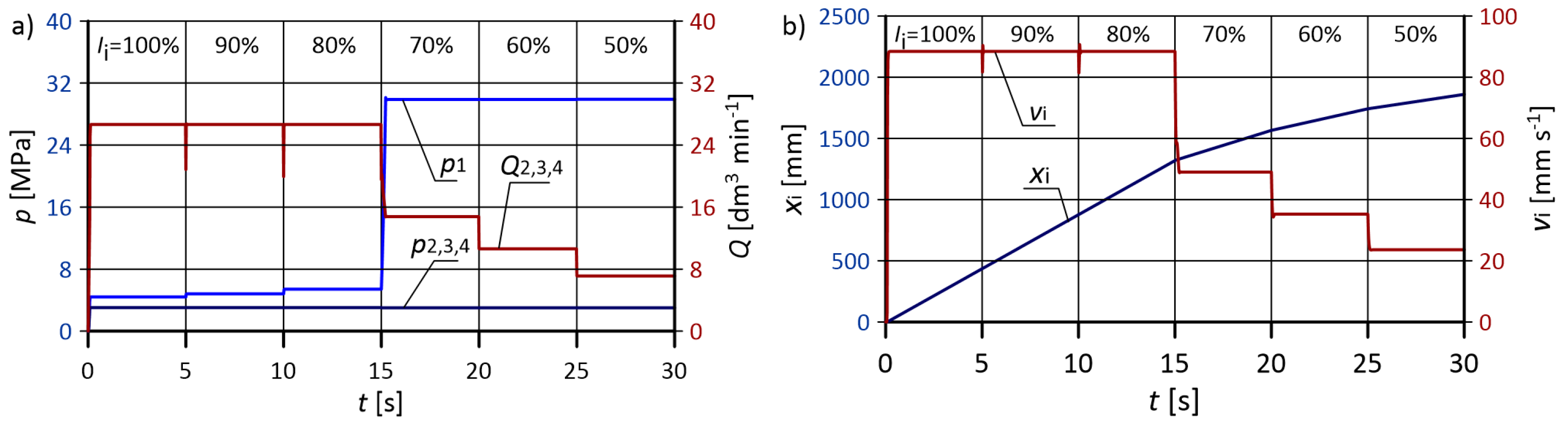
• equal actuator loads and fixed control signals for proportional valves,
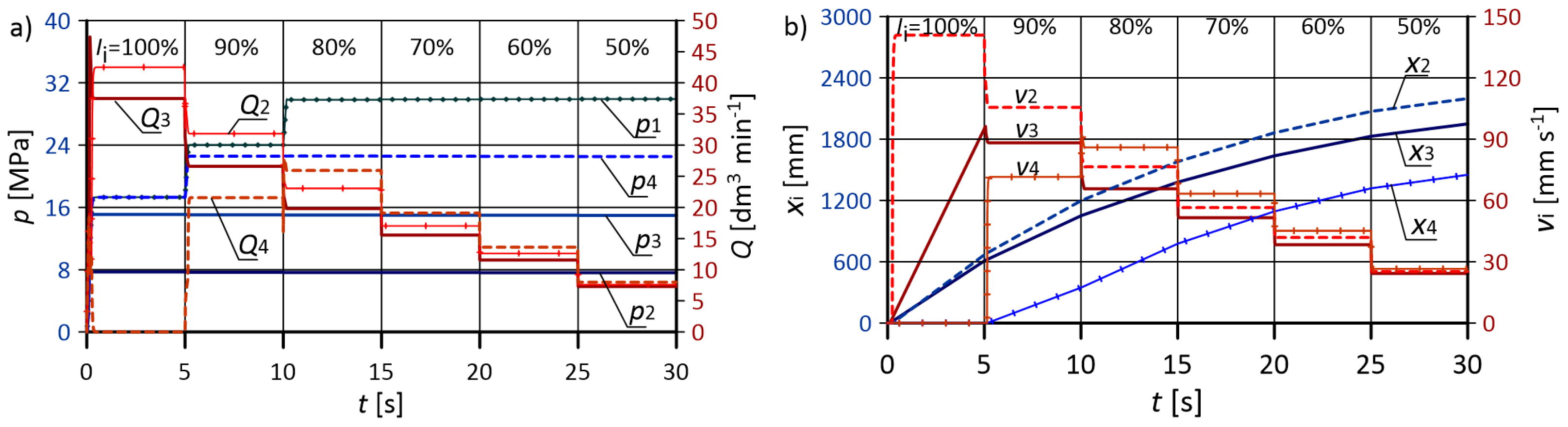
• various actuator loads and fixed control signals for proportional valves,
• proportional valve control for obtaining equal speeds of actuators with different loads.

In the first case, it was assumed that each actuator is loaded with the same force, while control signals for proportional valves, according to their characteristics obtained during the previous works [22], may vary in the range from $I_{min}=50$% to $I_{max}=100$% every $\mathsf{\Delta }I=10$%. Time series of parameters such as pressure, flow rate, displacement of actuator pistons were obtained and the total energy demand for each cycle was calculated for the load force: $F_{load,i}=15$, 50, 75, 100, 135 kN, which corresponds to the percentage values 10, 33, 50, 66, 90%, respectively. Exemplary results for the load $F_{load,i}=15$ kN are shown in Figure 6 (base system) and Figure 7 (LSB system). Analogous results for $F_{load,i}=135$ kN are presented in Figure 8 and Figure 9. The summary of total energy consumption determined for all considered cases is shown in

Table 3. Energy consumption, equal load force.

Load Force $F_{load,i}$ kN	15	50	75	100	135
Energy consumption—base, kJ	691.1	830.9	930.1	1028.7	1165.7
Energy consumption—LSB, kJ	183.3	457.7	654.3	850.9	1125.8
Relative reduction, %	73.5	44.9	29.6	17.3	3.4

.

As shown in Figure 6, if the load force in the base system is relatively low, and control signal $I_i$ is higher than the threshold value (70%), the whole pump flow rate is directed to the actuators and $p_1$ pressure is slightly higher than pressures in actuator lines. However, if the signal falls below the threshold, the supply line pressure is significantly increased to the value set on the relief valve. The energy loss is increasing and the flow rate is dropping rapidly. A similar phenomenon occurs at a high load force (Figure 8), however, in this case the energy losses are relatively lower due to the higher pressure in the actuator lines.

In contrast, the supply line pressure in the LSB system is slightly higher than the actuator line pressure regardless of the load force. Thus, energy loses are reduced. Additionally, the flow rate can be regulated throughout the range provided by the proportional valves. Thus, energy loses are reduced. Additionally, the flow rate can be regulated throughout the range provided by the proportional valves. The comparison presented in Table 3 shows that the LSB system allows a significant energy saving. The greatest savings, up to 70% may be achieved when the system operates at a minimum load. However, even with typical work cycles, a 20–30% reduction can be obtained.

In the second stage, the system with different actuator loads was tested. Figure 10 and Figure 11 show exemplary results obtained for $F_2=37.5$ kN, $F_3=75$ kN and $F_4=112.5$ kN (25%, 50% and 75% of the maximum load, respectively) in both the base system and the LSB system. The energy consumption for the different load cases is summarized in

Table 4. Energy consumption, different load forces.

Loads: $F_{load,2}$-$F_{load,3}$-$F_{load,4}$, kN	10-50-50	10-50-100	30-60-90	37.5-75-112.5	100-100-135
Energy consumption—base, kJ	828.5	1018.2	1014.3	1067.2	1124.3
Energy consumption—LSB, kJ	455.1	791.1	738.4	911.0	1084.0
Relative reduction, %	45.0	22.3	27.2	14.6	3.6

.

It can be noticed, that the courses of most parameters over time has similar form in both systems, except that the LSB ensures reduction in $p_1$ supply line pressure. Besides, if the proportional valve control signal is above 90%, the entire pump delivery is used by the less loaded actuators, while the most heavily loaded one is stationary. The comparison in Table 4 shows that during the execution of work cycles under typical loads (20–80% of maximum force), the LSB system can reduce the energy consumption up to 27%. Savings can be even higher in the case of low loads on all the actuators.

To date, the simulations have been carried out with the assumption of the same control signals for all proportional valves at a given time. As a result, the pistons under different loads moved at different speeds. In order to obtain equal speeds of all the actuators, it was necessary to appropriately adjust the values of the $I_i$ control signals. Hence, the third stage of the simulations consisted in obtaining the equal speed of the actuators at different loads by setting the control signals of the proportional valves. Load cases analogous to those used in the previous stage were studied. Figure 12 and Figure 13 show results for the case 4: $F_{load,2}=37.5$ unit kN, $F_{load,3}=75$ kN and $F_{load,4}=112.5$ unit kN and the expected piston speed $v_r=$ 60.0 mm/s.

Table 5. Energy consumption, different loads, equal speeds of all actuators.

Loads $F_{load,2}$-$F_{load,3}$-$F_{load,4}$, kN	10-50-50	10-50-100	30-60-90	37.5-75-112.5	100-100-135
Control signals $I_2$, $I_3$, $I_4$—base, %	79, 74, 74	78, 74, 70	77, 73, 71	76, 72, 68	70, 70, 66
Energy consumption—base, kJ	189.7	191.9	191.2	191.4	191.8
Control signals $I_2$, $I_3$, $I_4$ - LSB, %	70, 82, 82	71, 68, 82	72, 68, 83	73, 70, 83	69, 69, 84
Energy consumption—LSB, kJ	75.3	138.3	126.2	155.1	182.6
Relative reduction, %	60.3	28.1	34.0	18.8	4.7

presents the values of control signal set on the individual proportional valves and the energy consumption received.

The obtained results shown in Figure 12 and Figure 13 indicate that the assumed speed of the actuators was achieved in both, base and LSB system. In steady state, the maximum speed difference does not exceed $1.0$ mm · s⁻¹ However, the supply line pressure $p_1$ in the LSB system is approximately 20% lower and reaches the value of 24 MPa. Table 5 summarizes all the tested load cases with percentage values of the individual control signals and the energy consumption. The obtained results show that the reduction in energy consumption obtained by the LSB system compared to the base one is from $4.7$% to 60%, with an average value of 29%.

The presented solution is an innovative design of a load-sensing hydraulic system with respect to the state of the art. A comparison with other approaches to load-sensing systems is shown in

Table 6. Comparison of the features of load-sensing solutions.

Name, Publication	Additional Components	Geometrical Modifications	Advanced Control System	Hydraulic System Redesign	Avg/Max Energy Saving Ratio (%)
L-S for EHA pump [1]	Yes	Yes	No	No	n.a.
LSVCA [2]	Yes	No	Yes	Yes	efficiency improved $1.75$ times
L-S proportional valve [3]	No	Yes	No	No	n.a.
Stepper converter [4]	Yes	No	No	Yes	30%/60%
L-S for EHSS [7]	Yes	No	Yes	No	$62.5$%/90%
LS for excavator [9]	No	No	Yes	Yes	fuel saving over 20%
multi-DOF manipulator [10]	Yes	No	Yes	Yes	$25.8$%/$35.3$%
LS with reduced SIPL [12]	Yes	No	No	Yes	SIPL reduced by 44%
the studied LSB	Yes	No	No	No	29%/70%

. In particular, the following features indicate the novelty:

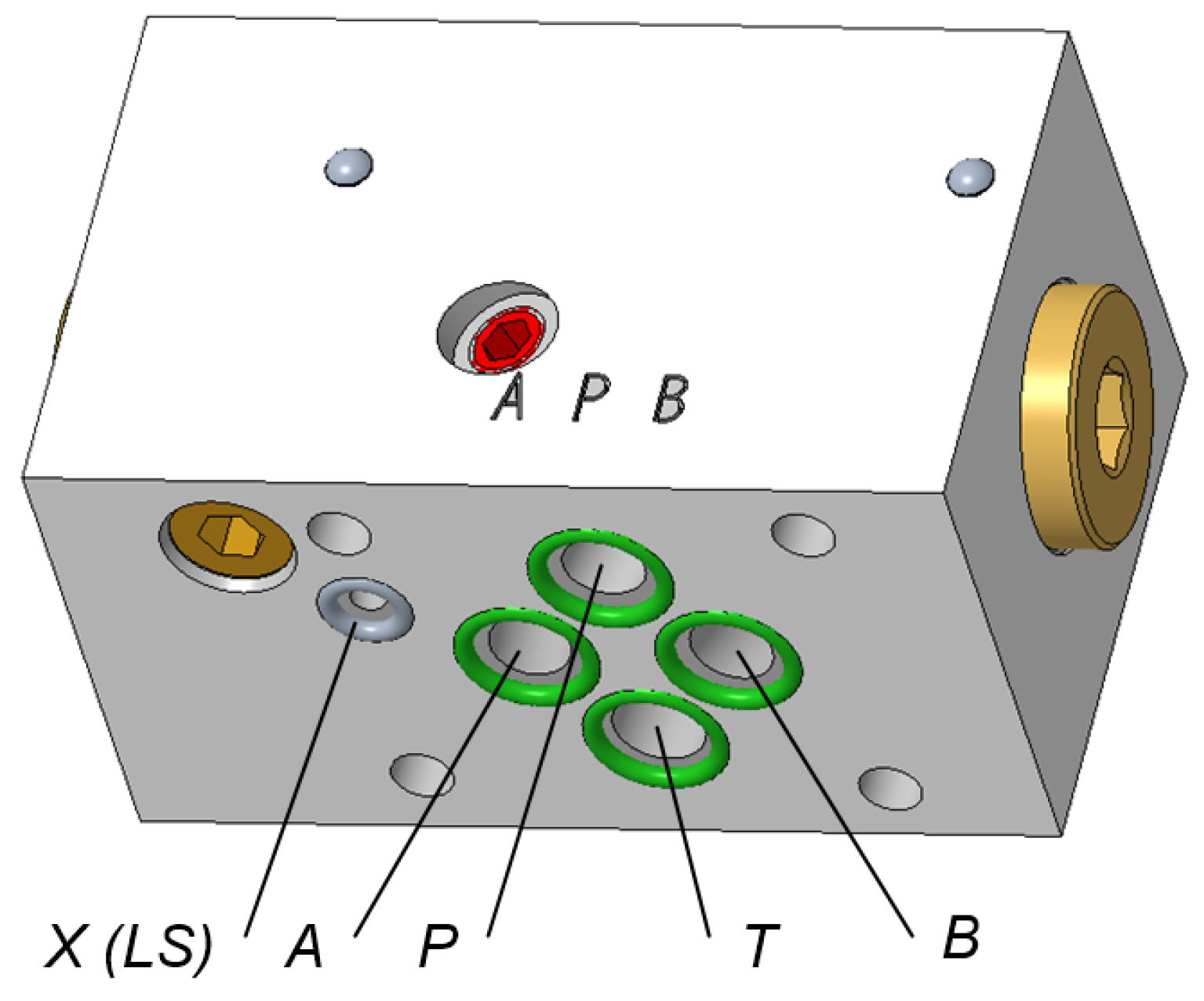
• although the load-sensing technique is generally well known, it has so far not been used industrially with ISO 4401 (formerly the CETOP standard) in a modular (sandwich) arrangement. Thus, the presented solution is an innovative application in industrial technology,
• the presented system is more universal than the currently used section valves due to the wide possibilities of expansion in a sandwich system by installing various types of valves and advanced configuration of individual sections,
• the number of actuators can be arbitrarily large, limited only by the pump capacity,
• unlike other solutions, only standard, typical hydraulic components were used. There is no need to modify them or use advanced electronic systems and control algorithms, which is crucial for the possibility of practical applications.

As arises from Table 6, the proposed LSB system needs additional hydraulic components, however, neither geometrical modifications, nor advanced control systems nor base system redesign are required. However, in practical applications some certain limitations must also be taken into account. The most important restrictions are:

• practical use is limited to components with ISO 4401 connectors (which means that it is dedicated to a specific type of connection according to the standard),
• the system can only work with distributors which, in their neutral position, relief A and B channels in order to send a proper signal to the load-sensing line (as shown in Figure 1).
• there is a necessity to use a hydraulic lock (double pilot-operated check valve) in the case when the actuator is loaded with force in the neutral position.

6. Conclusions

In typical industrial applications there are many simple, throttle-operated hydraulic systems controlled by directional or relief valves installed on a standard plate according to ISO 4401. It is a technologically feasible and relatively inexpensive solution. However, if multiple actuators are supplied from a single pump, significant energy losses can occur, particularly in the case when the actuators are loaded unequally. The article shows that the proposed load sensing system (LSB) composed of typical elements can be a beneficial solution ensuring significant energy savings. The LSB system, compared to conventional solutions, requires the use of an additional differential valve and information about the current load of the actuators. Typical logic valves and the ‘X’ port of the ISO plate were used to provide load information, based on the pressures in the individual actuator lines. The reduction of energy consumption was achieved by using a differential valve, also mounted on the plate. An important issue affecting the dynamical aspects of the system’s operation was the appropriate selection of the spring stiffness and the damping coefficient of the differential valve spool. In order to compare the LSB system parameters with a typical throttling solution, an appropriate model was built in the Simulink environment, taking into account the flow and motion equations, and a number of numerical analyses were carried out. Based on the obtained results, the following final conclusions were formulated:

• the presented solution is universal, the LSB system can be easily implemented as well as disconnected,
• the use of standard ISO plates is a convenient solution because it allows interchangeability of components from different manufacturers and easier configuration of control elements,
• the proposed system, depending on the load conditions of the actuators, allowed for energy savings from several to even 60–70%,
• the formulated mathematical model and the developed simulation model make it possible to quickly define various work cycles and assess the dynamics of the system and energy consumption in a given cycle,
• to obtain stable operation of the system, it is necessary to carefully select the spring stiffness and the damping coefficient of the spool in the differential valve,
• the use of an additional differential valve is associated with the appearance of some pressure losses, however, the benefits obtained from its use exceed this cost significantly,
• the proposed LSB system uses the currently available industrial design of a differential valve. In the future, research is planned to reduce pressure losses across the differential valve by optimizing the geometry of the spool and flow paths.

References

1. Chao, Q.; Zhang, J.; Xu, B.; Shang, Y.; Jiao, Z.; Li, Z. Load-Sensing Pump Design to Reduce Heat Generation of Electro-Hydrostatic Actuator Systems. Energies 2018, 11, 2266. [Google Scholar] [CrossRef] [Green Version]
2. Shang, Y.; Liu, X.; Jiao, Z.; Wu, S. An integrated load sensing valve-controlled actuator based on power-by-wire for aircraft structural test. Aerosp. Sci. Technol. 2018, 77, 117–128. [Google Scholar] [CrossRef]
3. Bigliardi, E.; Francia, M.; Milani, M.; Montorsi, L.; Paltrinieri, F.; Stefani, M. Multi-phase and Multi-component CFD Analysis of a Load—Sensing Proportional Control Valve. IFAC-PapersOnLine 2015, 48, 421–426. [Google Scholar] [CrossRef] [Green Version]
4. Gradl, C.; Scheidl, R. Performance of an Energy Efficient Low Power Stepper Converter. Energies 2017, 10, 445. [Google Scholar] [CrossRef] [Green Version]
5. Scheidl, R. The Hydraulically Controlled Oscillating Piston Converter. Energies 2021, 14, 2156. [Google Scholar] [CrossRef]
6. Pan, M.; Plummer, A.; El Agha, A. Theoretical and Experimental Studies of a Switched Inertance Hydraulic System in a Four-Port High-Speed Switching Valve Configuration. Energies 2017, 10, 780. [Google Scholar] [CrossRef] [Green Version]
7. Wang, W.; Wang, B. An Energy-Saving Control Strategy with Load Sensing for Electro-Hydraulic Servo Systems. Stroj. Vestn./J. Mech. Eng. 2016, 62, 709–716. [Google Scholar] [CrossRef]
8. Bedotti, A.; Campanini, F.; Pastori, M.; Riccò, L.; Casoli, P. Energy saving solutions for a hydraulic excavator. Energy Procedia 2017, 126, 1099–1106. [Google Scholar] [CrossRef]
9. Bedotti, A.; Pastori, M.; Casoli, P. Modelling and energy comparison of system layouts for a hydraulic excavator. Energy Procedia 2018, 148, 26–33. [Google Scholar] [CrossRef]
10. Ding, R.; Zhang, J.; Xu, B.; Cheng, M.; Pan, M. Energy efficiency improvement of heavy-load mobile hydraulic manipulator with electronically tunable operating modes. Energy Convers. Manag. 2019, 188, 447–461. [Google Scholar] [CrossRef]
11. Cheng, M.; Zhang, J.; Xu, B.; Ding, R. An Electrohydraulic Load Sensing System based on flow/pressure switched control for mobile machinery. ISA Trans. 2020, 96, 367–375. [Google Scholar] [CrossRef] [PubMed]
12. Siebert, J.; Wydra, M.; Geimer, M. Efficiency Improved Load Sensing System—Reduction of System Inherent Pressure Losses. Energies 2017, 10, 941. [Google Scholar] [CrossRef] [Green Version]
13. Novak, P.; Guinot, V.; Jeffrey, A.; Reeve, D.E. Hydraulic Modelling—An Introduction: Principles, Methods and Applications; CRC Press, Taylor & Francis Group: Boca Raton, FL, USA, 2010. [Google Scholar]
14. Kuehnlein, M.; Liermann, M.; Ewald, J.; Murrenhoff, H. Adjustable flow-control valve for the self-energising electro-hydraulic brake. Int. J. Fluid Power 2012, 13, 5–14. [Google Scholar] [CrossRef]
15. Milecki, A.; Rybarczyk, D. Modelling of an electrohydraulic proportional valve with a synchronous motor. Stroj. Vestn./J. Mech. Eng. 2015, 61, 517–522. [Google Scholar] [CrossRef]
16. Casoli, P.; Pompini, N.; Riccò, L. Simulation of an Excavator Hydraulic System Using Nonlinear Mathematical Models. Stroj. Vestn./J. Mech. Eng. 2015, 61, 583–593. [Google Scholar] [CrossRef] [Green Version]
17. Lisowski, E.; Filo, G. CFD analysis of the characteristics of a proportional flow control valve with an innovative opening shape. Energy Convers. Manag. 2016, 123, 15–28. [Google Scholar] [CrossRef]
18. Naseradinmousavi, P.; Nataraj, C. Nonlinear mathematical modeling of butterfly valves driven by solenoid actuators. Appl. Math. Model. 2011, 35, 2324–2335. [Google Scholar] [CrossRef]
19. Du, X.; Nydal, O.J. Flow models and numerical schemes for single/two-phase transient flow in one dimension. Appl. Math. Model. 2017, 42, 145–160. [Google Scholar] [CrossRef] [Green Version]
20. Antelmi, M.; Renoldi, F.; Alberti, L. Analytical and Numerical Methods for a Preliminary Assessment of the Remediation Time of Pump and Treat Systems. Water 2020, 12, 2850. [Google Scholar] [CrossRef]
21. Lisowski, E.; Czyżycki, W.; Rajda, J. Three dimensional CFD analysis and experimental test of flow force acting on the spool of solenoid operated directional control valve. Energy Convers. Manag. 2013, 70, 220–229. [Google Scholar] [CrossRef]
22. Lisowski, E.; Filo, G.; Rajda, J. Pressure compensation using flow forces in a multi-section proportional directional control valve. Energy Convers. Manag. 2015, 103, 1052–1064. [Google Scholar] [CrossRef]
23. Valdés, J.R.; Miana, M.J.; Núñez, J.L.; Pütz, T. Reduced order model for estimation of fluid flow and flow forces in hydraulic proportional valves. Energy Convers. Manag. 2008, 49, 1517–1529. [Google Scholar] [CrossRef]
Figure 1. Scheme of the analysed hydraulic system: 1—pump, 2—proportional control valve, 3—hydraulic cylinder, 4—hydraulic lock, 5—relief valve, 6—logic valve, 7—differential valve; black colour—base system, green colour—proposed LSB modification.
Energies 14 06735 g001
Figure 2. 3D model of the differential valve: 1—valve body, P, A, B, T, L S —connecting ports.
Energies 14 06735 g002
Figure 3. Longitudinal cross-section of the differential valve: 1—valve body, 2—spool, 3—spring, 4—damping nozzle; in, out—connecting ports, α / 2 —half of the cone opening angle, x 1 —spool position.
Energies 14 06735 g003
Figure 4. General scheme of the LSB simulation model in Simulink.
Energies 14 06735 g004
Figure 5. Differential valve subsystem in Simulink.
Energies 14 06735 g005
Figure 6. Results of the base system, equal load force F l o a d , i = 15 kN; (a) pressures and flow rates, (b) speeds and positions of actuators.
Energies 14 06735 g006
Figure 7. Results of the LSB system, equal load force F l o a d , i = 15 kN; (a) pressures and flow rates, (b) speeds and positions of actuators.
Energies 14 06735 g007
Figure 8. Results of the base system, equal load force F l o a d , i = 135 kN; (a) pressures and flow rates, (b) speeds and positions of actuators.
Energies 14 06735 g008
Figure 9. Results of the LSB system, equal load force F l o a d , i = 135 kN; (a) pressures and flow rates, (b) speeds and positions of actuators.
Energies 14 06735 g009
Figure 10. Results of the base system with variable load: F l o a d , 2 = 37.5 kN, F l o a d , 3 = 75 kN, F l o a d , 4 = 112.5 kN; (a) pressures and flow rates, (b) speeds and positions of actuators.
Energies 14 06735 g010
Figure 11. Results of the LSB system with variable load: F l o a d , 2 = 37.5 kN, F l o a d , 3 = 75 kN, F l o a d , 4 = 112.5 kN; (a) pressures and flow rates, (b) speeds and positions of actuators.
Energies 14 06735 g011
Figure 12. Results of the base system with variable load: F l o a d , 2 = 37.5 kN, F l o a d , 3 = 75 kN, F l o a d , 4 = 112.5 kN and the required piston speed v i = 60.0 mm/s; (a) pressures and flow rates, (b) speeds and positions of actuators.
Energies 14 06735 g012
Figure 13. Results of the LSB system with variable load: F l o a d , 2 = 37.5 kN, F l o a d , 3 = 75 kN, F l o a d , 4 = 112.5 kN and the required piston speed v i = 60.0 mm/s; (a) pressures and flow rates, (b) speeds and positions of actuators.
Energies 14 06735 g013