DC-Link Capacitor Diagnosis in a Single-Phase Grid-Connected PV System

Abstract

The DC-link capacitor is one of the components that are more prone to faults in energy-distributed systems based on voltage source inverters. A predictive maintenance approach should allow to foresee the risk of an unexpected system shutdown. In this study, a two-stage diagnostic approach that is aimed at determining the health status of the DC-link capacitor in a single-phase grid-connected PV system was proposed. The equivalent series resistance (ESR) and the capacitance (C) values were used as indicators in the estimation of the degradation stage. Electrochemical impedance spectroscopy (EIS) was used to estimate the impedance curve of the DC-link capacitor, and a multi-fitting algorithm allowed us to determine the ESR and C parameters. A comparison between the estimated values C and ESR and the nominal values was used to quantify the fault severity. It was demonstrated that the EIS allowed the determination of the capacitor impedance regardless of the actual operating conditions of the photovoltaic generator, such as during irradiance changes and with the maximum power point algorithm turned off. By using the capacitor simplified model and a multi-fitting algorithm, the C and ESR values were estimated with an error that was lower than 1%. An analysis of the hardware required to implement the proposed approach in real applications by achieving the desired accuracy was also proposed.

1. Introduction

Power converters are critical elements that convert the power generated from different sources to useful power to consumers in several applications. In distributed energy systems and microgrids, faults or failures in power converters could produce instabilities and affect the quality and the reliability of the energy service. The main faults occurring in power converters are related to capacitors and power switches, namely the 50% and 30% of the total, respectively [1]. The operation of such components is affected by a number of operating and exogenous factors [2]. In the former group, overvoltage stress, excess ripple current, and repeated charge/discharge cycles are the main causes of faults. For example, in photovoltaic and wind systems, the continuous changes of solar irradiance and the wind speed profiles, as well as the ambient temperature, have a significant impact on the ripple current stress of DC-link capacitors of inverters. As for the environmental factors, the high ambient temperature and humidity have the more relevant effect. Indeed, the major degradation of metallized film capacitors occurs in applications exposed to high humidity environments. The primary failure mechanism of electrolytic capacitors is due to the thermal stress [2].

Lifetime indicators play an important role to determine the health status of capacitors, thereby helping to prevent unexpected shutdowns. In the literature, equivalent series resistance ($ESR$), capacitance C, ripple voltage, volume, and temperature are the proposed lifetime indicators for capacitor monitoring. The $ESR$ is related to the AC losses; the capacitance expresses the capability to store energy; the volume relates to the electrolyte; and the temperature is the capacitor core temperature [2,3,4]. Health indicators depend on environmental and electrical conditions, and since the capacitor is essentially an electrochemical device, the different indicators are closely related. For example, in thermal overload situations, the electrolyte may evaporate, so the $ESR$ increases and C decreases. The same events happen in conditions of overvoltage stress or excessive ripple current in a continuous way. On the other hand, high temperature produces an increase in the internal pressure of capacitor, which changes the capacitor volume and/or gives rise to losses inside the electrolyte [2]. Moreover, in [5] it has been demonstrated that $ESR$ failures may have dynamics that are faster than the C ones, depending on the capacitor technology. Although in some studies only one indicator is used to study the capacitors degradation, the previous remarks put into evidence that the estimation of both indicators (C and $ESR$) provides a more accurate degradation detection. The measurement of non-electrical indicators, such as temperature and volume, requires thermography, acoustic analysis, X-ray imaging, weighing, or optical inspection approaches [6]. This makes the adoption of such indicators uncomfortable in online applications, with respect to the measurement of $ESR$ and C current values.

According to [3], the latter indicators are the best to perform online diagnosis. They are clearly linked with the capacitor life status. A significant increase in $ESR$ may indicate an incoming catastrophic event [7]. In aluminum electrolytic capacitors, the widely accepted end-of-life criterion is a 20% capacitance reduction or an $ESR$ doubling. As for film capacitors, a reduction of 2% to 5% of the capacitance value may indicate the end-of-life [8].

The frequency domain analysis is the most-used approach to measure capacitance and $ESR$ values. The impedance curve of an electrolytic capacitor at a fixed temperature is shown in Figure 1. The regions at low and at high frequency, i.e., Z${}_1$ and Z${}_2$, are dominated by the capacitive reactance and by the equivalent series resistance, respectively. Meanwhile, in the third zone, i.e., Z${}_3$, the inductive impedance of the capacitor prevails. The frequencies ($f_a$ and $f_b$) depend on the capacitor technology [6]. The black line and the dotted blue line shown in Figure 1 sketch the frequency responses of a new and of a degraded capacitor, so that the increment of ESR in the second case is made evident.

In the literature, several methods for estimating the capacitor parameters during their operation in power converters have been proposed. The main differences among these approaches are: the number of estimated parameters, the amount of measures required, and the estimating technique. Unfortunately, only a few approaches can be used online [3]. In spite of the previous described correlation among the two electrical indicators C and ESR, in some studies, e.g., in [9,10], only the $ESR$ is estimated. In [9], the $ESR$ of the DC-link capacitor of a boost converter is determined by measuring the capacitor voltage and the inductor current peak by using a suitable ripple voltage extraction circuit. Wavelet transform denoising allows to determine accurately the current peak when white, random, and repetitive pulse-shaped noises affect the signal. An acquisition system working at a high sampling frequency (10 MHz) is used. In [10], a Rogowski sensor was adopted to measure the inductor voltage and the current of a buck converter. The $ESR$ estimation also requires that the capacitance value and the sensor mutual inductance value are known.

The approaches presented in [11,12,13,14] allow the estimation of $ESR$ and C indicators, in a one-stage buck or boost converter, at the price of a high number of measured signals and of the need of computationally expensive estimation techniques. In [11,12], a buck and a boost converter for power factor correction were analyzed. In both cases, the capacitor voltage ripple measurement, in two specific instants, was required. In [11], the switching frequency, the duty cycle, and the inductance values must also be determined. In [12], the frequency and power grid values were needed. The capacitor ripple voltage affects the estimation accuracy; thus, the required hardware included an isolated amplification circuit and a trigger circuit to acquire the PWM signal, so that a transformer magnetic core is employed. Additionally, the trigger circuit must be adjusted according to duty cycle changes. The computational burden is not relevant.

More complex estimation techniques are presented in some other studies. In [13], the boost converter output capacitor diagnosis needs the measurement of the inductance current, the capacitor voltage, and the PWM signal. Moreover, the boost converter model is used to implement a particle swarm optimization algorithm to determine, in a stochastic way, the capacitor parameters. In [14], a state-observer was involved to estimate the capacitor health indicators in a buck converter. By introducing a 100-Hz perturbation of the set-point, the capacitor output voltage was perturbed as well. This affected the inductor current waveform. The capacitor C was estimated by integrating the difference between the estimated and the measured capacitor voltage. The $ESR$ was determined by measuring the capacitor voltage, while the current was calculated by using the measured load and the inductor current.

Besides, in distributed energy systems and microgrids, a cascade of converters is typically required. Moreover, LCL filters and synchronization circuits are often used in grid-connected solutions. Consequently, significant circuit-to-circuit correlations, at different operating and environmental conditions, arise. In PV DC/DC converters used for battery charging and in general DC applications, the capacitors mainly adsorb the switching ripple, with an amplitude that is a fraction of the converter nominal current. Instead, the DC-link capacitor used in single phase grid-connected power processing systems absorbs a large current, allowing it to compensate the fluctuating power injected into the grid [15]. Such greater stressing operating conditions lead to accelerated DC-link capacitance degradation. Therefore, in grid-connected systems, because of the large number of phenomena or elements affecting the capacitor operation, the online estimation of the C and $ESR$ values has to be performed more carefully, if a reliable capacitor state-of-health is desired. The online estimation of the capacitor degradation, during its normal operation, requires the acquisition of some voltage and current waveforms, including the ripple and the noise affecting them. In [16], the online estimation of the capacitance value of the output capacitor in a phase-shifted H-bridge converter was performed through the injection of a signal at 50 Hz. The method requires the measurements of the output voltage, of the load current, and of the secondary-side DC-link current. In [17], a perturbation signal was added to the current control of the inverter stage in a cascaded AC/DC/AC scheme. The injected perturbation signal was at 30 Hz, thus at a frequency that is lower than the line one. The technique allows the estimation of the current capacitor from measured line currents, by determining the midpoint of those ones in a switching period. The measured voltage and the estimated current capacitor are used to obtain the $ESR$ value. In [18] a capacitance estimation scheme in a PV H5 inverter by using a 30-Hz perturbation signal was proposed. This online method requires specific values of DC-link voltage and PV-current during the zero-state of the inverter.

In [19], a capacitor impedance estimation scheme in a grid-connected single-phase H bridge inverter was proposed. This online method measures the DC-link voltage and reconstructs the capacitor current by using the inverter output current and the PWM signal. Then, the second harmonic ripple current and the capacitor voltage are extracted by using the SOGI filter. Finally, the capacitor impedance is estimated by using the filtered signals. In [20], the estimation of $ESR$ and C indicators of the DC-link capacitors in a bank of an on-grid PV system is presented. By measuring the PV current, the grid side current, and the PWM signal, the current of the bank was determined. An LCR meter was required to calibrate the initial C and $ESR$ values of the bank and each capacitor therein. A physics-of-failure-based degradation model was proposed to determine the core temperature of each capacitor, assuming that each one exhibited the same degradation rate. An extended Kalman filter algorithm was used to update that model. Finally, the $ESR$ and C of each capacitor were estimated by using a least-mean-square optimization algorithm.

The estimation error affecting both C and $ESR$ indicators when the previously described techniques are used is presented in

Table 1. Features of the methods proposed in literature.

Reference Number	{C, ESR} Estimation Error	Comments
[16]	C: 2.5–4%	Technique customized for a phase-shift full-bridge DC–DC converter.
[17]	ESR: 3.2%	Needs the injection of a current stimulus. Operates in no-load condition.
[18]	C: 1.5%	Technique customized for the H5 inverter.
[19]	Z: 17.2%	Does not provide C and ESR separate estimations.
[20]	ESR: 2.14% C: 0.19%.	Requires LCR meter to provide initial values of C and ESR of each capacitor of a bank.

. In the literature, studies [16,17,18,19] propose methods to estimate one indicator only, where the best precision achieved was 1.5% in the capacitance. The technique described in [20] is the only one estimating both the parameters but with a higher $ESR$ estimation error and by requiring special equipment to determine the initial value of C and $ESR$. Some diagnosis techniques of the capacitor have been proposed for specific topologies of converters, such as [16,18]. The technique proposed in [16] works exclusively for a DC/DC conversion topology, which is without inversion stage. Another aspect to highlight in diagnosis methods is related to the impact in the normal operation of the system. The method proposed in [19] does not require to stop the system—even a current sensor of capacitor is not needed—but only the whole impedance of the capacitor is estimated with a large error. In contrast, the method proposed in [17] provides a better estimation error, but that technique affects the normal operation of the system, because a current injection in a no-load condition is required. A comparison analysis of those results in the literature with the ones obtained through the proposed approach is included in Section 5 of this article.

In this study, a method for the online diagnosis of the DC-link capacitor in a single-phase grid-connected PV system was proposed. The proposed approach consists of two stages: the estimation of the degradation indicators and the threshold comparison procedure. In the former step, the capacitor impedance is estimated through the EIS. Afterwards, a multifitting algorithm allows to identify the $ESR$ and C values. Finally, the diagnosis is based on the comparison of the identified values with the corresponding nominal values, thus enabling an alarm produce. The proposed approach shows a good trade-off between the computational burden and the parameters’ identification accuracy. It requires a simple system for the acquisition of signals needed for its implementation. The proposed EIS-based method allows to estimate the capacitor state-of-health during the normal operating conditions of the PV generator, thus also during irradiance transients and by switching off the maximum power point tracking algorithm. The technique was implemented by using standard voltage and current sensors and a low-cost processor, e.g., the BeagleBone Black. Thus, the high performance and expensive hardware required for implementing other techniques presented in the literature was not needed. Additionally, the computational burden of the proposed technique fits with low-cost processors that are actually available on the market.

In Section 2, the model of the electrolytic capacitor employed in this article is presented and two different methods for estimating the parameters of the capacitor are summarized. In Section 3 the proposed electrochemical impedance spectroscopy (EIS)-based diagnostic method is described. In Section 4, the proposed diagnostic method is applied to the selected case of study, and validation and implementation issues are analyzed. Section 5 discusses the results obtained by means of the proposed EIS method, by taking into account the hardware requirements. Finally, conclusions and perspectives for future activities end the article.

2. Electrolytic Capacitor Modeling

Electrolytic capacitors are used in PV systems to filter noises, to smooth the converters switching’ frequency ripple, and to stabilize the DC bus voltage [21]. The higher energy density and the lower cost with respect to film capacitors make them suitable for many applications [22]. Consequently, in this study, an electrolytic DC-link capacitor used in a single-phase grid-connected PV system was considered as the subject of the study.

In the literature, some models representing the behavior of electrolytic capacitors are presented. Some examples are presented in Figure 2. The estimation of their parameters requires that the following three issues must be kept into account: manufacturer capacitor circuit model, temperature dependence, and frequency dependence [23]. They are briefly summarized here below.

Manufacturer Capacitor Circuit Model: the aluminum electrolytic capacitors models presented in Figure 2 include the following parameters:

• $C_i$ is the ideal capacitance.
• $R_P$ is the parallel resistance, which represents all the losses in the dielectric and the leakage between the two electrodes.
• $R_S$ is the connection and electrode serial resistance.
• $L_S$ is the connection and winding equivalent series inductance.
• D diode represents the rectifying property of the oxide dielectric, which is similar to the PN junction in semiconductor devices.
• $C_D$ is the inherent dielectric absorption.
• $R_D$ is the dielectric loss due to dielectric absorption and molecular polarization.

Temperature Dependence: temperature affects the parameter values of a capacitor. The $ESR$ decreases as the operating temperature increases, because of the increased conductivity of the electrolyte [23]. Instead, the capacitance value increases. A temperature decrease leads to the capacitance reduction; frequency characteristics of the $ESR$, impedance, and capacitance are also affected [26].

Frequency Dependence: the capacitor impedance (1) puts into evidence the dependence from the operating frequency $\omega$. In power converters, the switching frequency usually can vary from tens of kilohertz to a few megahertz [27]. Therefore, in Equation (1), the equivalent series inductance ($ESL$) is very small compared to $ESR$, so usually it is neglected [28]. Consequently, as it is shown in Figure 3, the model of electrolytic capacitors used in power converters can be simplified by including two parameters only, i.e., capacitance (C) and ESR.

$$\left|Z\left(\omega \right)\right|=\sqrt{ES{R}^2+{\left(ESL\omega -\frac{1}{C\omega }\right)}^2}$$

(1)

In this study, the simplified capacitor model shown in Figure 3, in which the temperature effect is neglected, was considered. Therefore, the capacitor health state was assessed through the estimation of the $ESR$ and of the capacitance C values.

Capacitor Parameters Estimation Methods

In the literature, some methods to estimate capacitor parameters have been proposed [29,30,31]. They are aimed at measuring and then processing the voltage ripple and the capacitor current. In the following, the two main used methods are briefly introduced.

Ohmic frequency range method. The $ESR$ parameter is calculated by evaluating the voltage/current relationship [30], thus by measuring the capacitor voltage ($V_{out}$) and current $I_{ESR}$. The estimation is done in the capacitor’s ohmic frequency range, i.e., around the switching frequency of the power converter. $V_{out}$ and $I_{ESR}$ signals are filtered by using a band-pass filter; then, the RMS to DC block (integrated circuit) converts the $V_{out}$ and the $I_{ESR}$ signals into a equivalent DC current. The ratio of the processed signals gives the $ESR$ value. In this approach, the capacitance value is not calculated, although it is a useful parameter for assessing the capacitor state of health.

Capacitor power losses method. This approach [29] avoids an extensive filtering action by calculating power losses in AC. Signals $V_{out}$ and $I_{ESR}$ are measured, even by employing a Rogowski coil as a current sensor. The ripple affecting the signals is extracted and processed to calculate the power $P_C$, thus determining the $ESR$ value as it is indicated in Equation (2). Unfortunately, this method does not allow to estimate the capacitance value.

$$ESR=\frac{P_C}{{I_{ES{R}_{AC}}}^2}$$

(2)

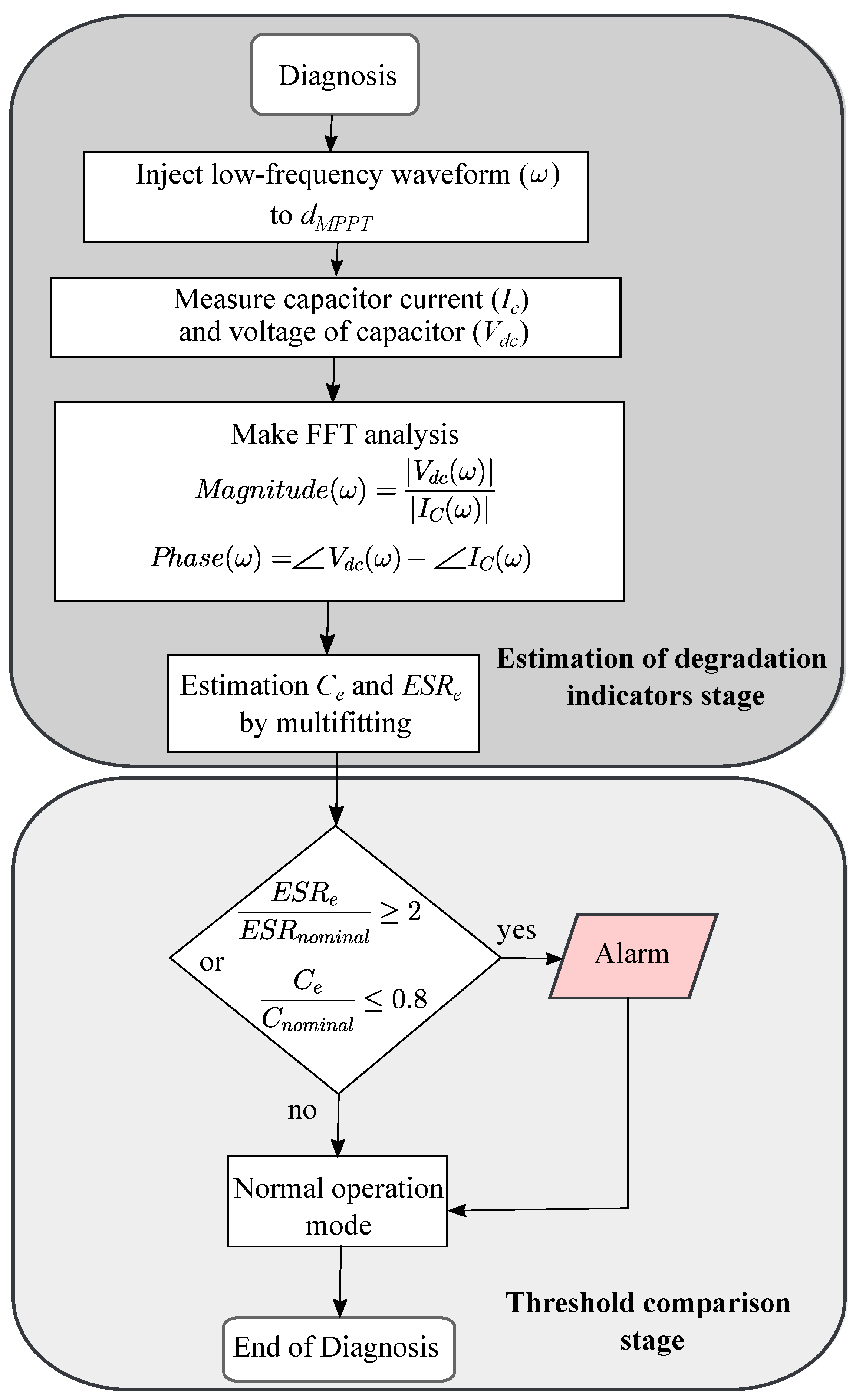
3. DC Link Capacitor Diagnosis by Means of Electrochemical Impedance Spectroscopy (EIS) and Data Multi-Fitting

EIS is a widely used approach [31] that allows to calculate the impedance value by using the relation (3) between current and voltage signals measured.

$$Z\left(\omega \right)=\frac{V\left(\omega \right)}{I\left(\omega \right)}$$

(3)

In the PV context, the EIS method has been used to determine the model of a PV panel, which is connect at a boost converter input to perform the maximum power point tracking (MPPT) function [32]. A small sinusoidal perturbation of a controlled amplitude and frequency is applied, and the current and voltage signals at the PV generator are measured. In [32], the frequency injection is performed online by operating through the PWM control of the boost converter, which operates in continuous-conduction mode. The switching frequency is 100 kHz, and frequency injection runs from 500 Hz until 90 kHz. To inject low-frequency pulses in conjunction with the normal higher frequency pulses associated with the boost converter operation, the duty cycle is modified according to (4).

$$d\left(t\right)=d_{MPPT}+A_{d}sin\left(\omega t\right)$$

(4)

where:

• $d_{MPPT}$ is the duty cycle of the MPPT control.
• $A_d$ is the perturbation amplitude.
• $\omega =2\pi f_{EIS}$ is the low-frequency component.

The proposed diagnostic method uses the EIS approach, and it consists of two stages, which are named estimation of degradation indicators and threshold comparison. The indicators used to assess the capacitor state-of-health are its ESR and its capacitance C. If the capacitance value is decreased by 20% of the nominal value and/or the ESR is doubled with respect to the nominal value, the capacitor is considered damaged and must be changed [4]. In the following, the two stages of the proposed diagnostic procedure are described.

Estimation of degradation indicatorsCandESR. In Figure 4, the procedure for estimating the values of the two indicators is described. The first step aims at estimating the capacitor impedance plot, i.e., magnitude and phase, by using the EIS. In the second step, a multi-fitting algorithm is used to determine the values C and $ESR$ by fitting the capacitor model with the online measured magnitude and phase curves. The perturbation signal needed to perform the EIS is injected through the converter modulator at different frequencies $\omega$. The DC-link voltage and the capacitor current are measured; thus, their magnitude and phase at each injected frequency value are calculated by performing an FFT operation.

Threshold comparison. In this stage, the current values of the estimated indicators $C_e$ and $ES{R}_e$ are compared with the nominal values $ES{R}_{nominal}$ and $C_{nominal}$, which are available in the capacitor datasheet. That comparison is made by calculating the relationships $\frac{ES{R}_e}{ES{R}_{nominal}}$ and $\frac{C_e}{C_{nominal}}$, which must be lower to 2 or higher to 0.8, respectively, for a non-degraded condition of capacitor. The selected thresholds, i.e., 2 and 0.8, are the recommended values taken from the literature [4].

4.  Validation and Implementation Issues

In this section, the proposed technique, which has been described previously, is validated by referring to the DC-link capacitor of an on-grid PV system. The case of study is firstly described in detail. Then, the configuration of the perturbation signal to be injected into PWM is discussed. Afterwards, the capacitor frequency domain model and the fitting procedure to determine C and ESR indicators are presented. Finally, in this section, the hardware requirements for implementing the proposed technique are explained in depth.

4.1. System Description and Parameters Configuration

In Figure 5, the DC-link capacitor of a single-phase grid-connected PV system is put into evidence. A boost converter running the perturb and observe MPPT technique is the first stage shown in Figure 5. The converter connects a 1800-W PV array to an inverter connected to the 240-V grid. The inverter control consists of current and voltage control laws and of an inner feedforward loop, as it is shown in Figure 6.

The PV array is formed by seven series-connected Trina Solar TSM-250 modules. The specifications of each module are: 60 series-connected cells, open-circuit voltage $V_{oc}$ of 37.6 V, short-circuit current $I_{sc}$ of 8.55 A, and voltage and current at maximum powers ($V_{mpp},I_{mpp}$) of 31 V and 8.06 A, respectively.

Table 2. Boost converter and inverter parameters.

Parameter	Variable	Value	Units
Switching frequency of boost	$F_{sw}$	20	kHz
Carrier frequency of inverter	Fc	3780	Hz
Inductor	L	5	mH
Output capacitor	C	2200	$\mathsf{\mu }$F
Equivalent series resistor	$ESR$	114.5	m$\mathsf{\Omega }$
Input capacitor	$C_{input}$	100	$\mathsf{\mu }$F
Resistor of inductance (LCL filter)	$r_f$	8.23	m$\mathsf{\Omega }$
Inductor (LCL filter)	$L_f$	2.18	mH
Resistor of capacitance (LCL filter)	$r_c$	2.193	$\mathsf{\Omega }$
Capacitor (LCL filter)	$C_f$	24	$\mathsf{\mu }$F

lists the parameters of the boost converter, of the inverter, and of the LCL filter. The parameters of the boost converter are those ones of the same converter available at the test-rig microgrid developed at Laboratorio de Accionamientos Electricos and Electronica de Potencia of Universidad del Valle. The switching frequency of the boost converter was 20 kHz; the parameters $\delta D$ and $T_a$ of the Perturb and Observe algorithm were settled according to the recommendations given in [33].

The single-phase inverter converts 400VDC to 240VAC and uses the PWM bipolar modulation method at a carrier frequency of 3780 Hz. Figure 6 shows the inverter control scheme, where the voltage control loop regulates the DC link voltage at 400 V and determines the reference Id (active current) required by the current regulator. The reference Iq (reactive current) was set to zero. Besides, LCL filter parameters and grid current and voltage signals were used by the feed-forward control loop. Figure 7 shows the phasel-Locked loop (PLL) synchronization unit of the inverter with the grid and the single-phase dq transform. The grid was modeled using an ideal AC source of 240 V RMS nominal voltage at 60 Hz.

At first, the whole system was simulated in order to show its ordinary operating conditions without applying the diagnostic action. The PV array operated at (25 °C, 400 W/m²). Figure 8 shows the following waveforms: the DC-link voltage (green line), the duty-cycle of MPPT of the boost converter (black line), the PV array power (brown line), and irradiance (blue line). The sequence of events are:

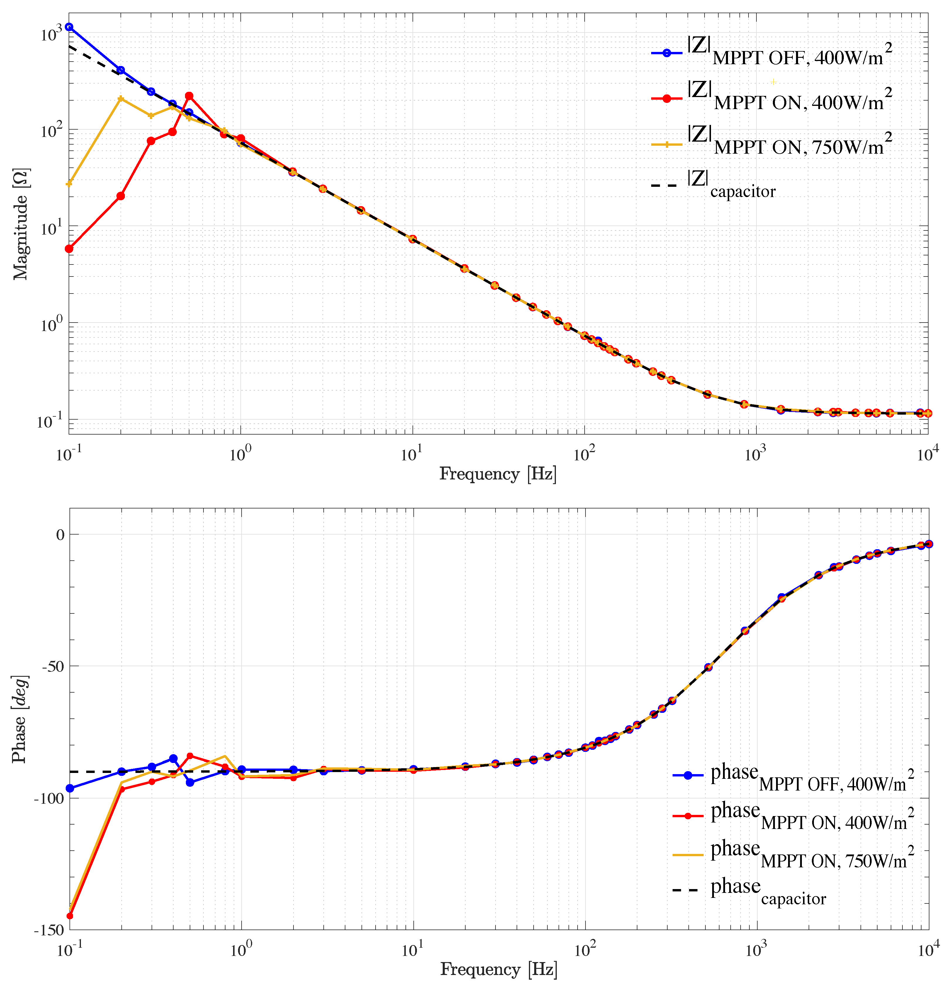
• From t = 0 s to t = 0.5 s, the duty-cycle of the boost converter was fixed at D = 0.4. In order to ensure a stable state of DC-link, the MPPT algorithm was disabled.
• At t = 0.5 s, MPPT was enabled. The MPPT algorithm varies the duty-cycle to extract maximum power. The PV array output power was 694 W at 400 W/m² and 25 °C. It observed the regulation of DC-link voltage.
• At 2.5 s, the irradiance was changed to 750 W/m², and the temperature remained at 25 °C. The power developed by the system was increased to 1312 W. The DC-link voltage and the duty-cycle, which are controlled by the MPPT algorithm, were subjected to a transient.

4.2. Injection of Sweep-Frequency into PWM of Boost Converter to Develop the EIS Test

The EIS method presented in Section 3 was applied to the previously simulated system in order to determine the impedance of the DC-link capacitor. It was measured at two different irradiance values, i.e., 400 W/m² and 750 W/m², by turning off the MPPT algorithm in the former case. The temperature was fixed at 25 °C. The EIS perturbation amplitude was set to 5% of the nominal duty cycle value (i.e., $A_d=0.022$), and the perturbation frequency was swept between 0.1 Hz and 10 kHz. Voltage and current sensors were used to measure $Vdc$ and $I_C$ at the DC-link capacitor. Then, the magnitude and the phase of $Vdc$ and $I_C$ were obtained by using the FFT Matlab function for each one of the perturbation frequencies ($f_{EIS}$).

In order to perform a suitable FFT analysis, the sampling frequency and the number of data must be balanced. In general, high sampling frequencies are preferable, but the cost is a high number of data to be stored and processed, so more memory and computation time are required. The problem is more critical in the low frequency range, where more time is required to obtain enough data and where the harmonics have a very small amplitude due to the high impedance of the capacitor [34].

At the first stage, limitations concerning the sensors and the acquisition systems were neglected. Their optimization is described more later in this article. Thus, initially, the sampling frequency was settled at 756 kHz, which corresponds to 200 times the carrier frequency of the inverter. Using ten values per decade between 10 Hz and 10 kHz, and other well-spaced values at frequencies lower than 10 Hz, a total of 44 different sinusoidal stimuli at 44 $f_{EIS}$ frequencies were injected through the converter PWM control. Figure 9 shows the results of the estimated magnitude and phase of the capacitor impedance in different operating conditions. In order to allow the comparison between the estimated impedance and the real behavior, the known curve of the impedance capacitor was added as a dotted black line. The blue line corresponded to the calculated impedance when the MPPT was disabled and the irradiance value was 400 W/m². Meanwhile, the red and yellow lines are the results when the MPPT was enabled and the irradiance value was equal to 400 W/m² and 750 W/m², respectively. It is evident that the EIS method allowed us to estimate the magnitude and phase of the DC-link capacitor impedance in those different operating conditions, at least for frequencies that were higher than 1 Hz. Nevertheless, this first simulation demonstrates that the injection of stimuli at frequencies ranging from 1 Hz until the half of the switching frequency $F_{sw}$ allowed us to correctly estimate the impedance of the DC-link capacitor.

4.3. Multiple Curve Fitting Algorithm to Determine C and ESR

The magnitude and phase curves that are measured through the EIS are used to estimate the two parameters, C and $ESR$, through a multi-fitting algorithm, i.e., the NLINMULTIFIT function, which operates a NonLinear Least Squares Regression of multiple data sets [35]. The NLINFIT Matlab function operates the simultaneous fitting of multiple non-linear curves with shared parameters. Equations (5) and (6) show the magnitude ($|Z_{EIS}|$) and the phase (${\theta }_{EIS}$) equations of capacitor that have been used in the fitting procedure, where $\omega =2\pi f_{EIS}$. The data measured at frequencies that are lower than 1 Hz have been excluded from the fitting procedure because of their inaccuracy (see Figure 9).

$$\left|Z_{EIS}\right|=\sqrt{ES{R}^2+{\left(-\frac{1}{\omega C}\right)}^2}$$

(5)

$${\theta }_{EIS}={tan}^{-1}\left(\frac{-1}{\omega CESR}\right)$$

(6)

The output of the multi-fitting procedure is presented in

Table 3. Estimation of C and ESR indicators for non-degraded and degraded capacitor cases.

	Nominal			Degraded
	ESReN (mΩ)	CeN (μF)	MSEN	ESReD (mΩ)	CeD (μF)	MSED
MPPT OFF, 400 W/m2	114.07 ± 0.719	2188 ± 10.99	1.030	228.78 ± 0.709	1759 ± 4.69	1.028
MPPT ON, 400 W/m2	114.80 ± 0.767	2183 ± 11.64	1.0301	228.76 ± 1.25	1758 ± 8.28	1.0281
MPPT ON, 750 W/m2	114.66 ± 0.036	2201 ± 5.57	1.0308	228.96 ± 1.20	1757 ± 7.97	1.030
Expected Values	114.5	2200		229	1760

. Degraded and non-degraded capacitor cases were considered. In order to simulate the degraded capacitor case, the $ESR$ and C values were changed by 80% and 100%, respectively. Both the operating conditions with different irradiance levels, i.e., 400 W/m² and 750 W/m², and the turning off of the MPPT algorithm were also considered in this case. The DC-link capacitor installed in the experimental test bed was a Nippon U36D series at 450 V, and its nominal $ESR$ and C values provided by the manufacturer were 114 m$\mathsf{\Omega }$ and 2200 $\mathsf{\mu }$F, respectively [36]. The guess conditions used for the multi-fitting algorithm in the non-degraded case were fixed at $ES{R}_{0_N}=50$ m$\mathsf{\Omega }$ and $C_{0_N}=1500$ $\mathsf{\mu }$F; thus, they are far from the nominal values. Instead, the nominal values $ES{R}_{0_D}=114$ m$\mathsf{\Omega }$ and $C_{0_D}=2200$ $\mathsf{\mu }$F were used as a guess solution for the fitting in the degraded case. The parameters of the multifitting algorithm were settled as it is shown in

Table 4. Parameterization of multifitting algorithm.

Parameter	Type or Value
Method	NonLinearLeastSquares
Weight function for robust fitting	Bisquare
DeviStep	$ep{s}^{1/3}$
MaxIter	200
TolFun	$1\times {10}^{-8}$
TolX	$1\times {10}^{-8}$

: the termination tolerance on estimated coefficients (TolX) and the residual sum of squares (TolFun) were set to $1\times {10}^{-8}$. The maximum number of iterations to stop the estimation (MaxIter) was settled at 200. The value $epsilo{n}^{1/3}$ was used for the relative difference for the finite difference gradient parameter (DeviStep). From Table 3, it results that the mean square error (MSE) of the fitting process was close to 1; so, a very good estimation accuracy was reached. For determining the parameters’ confidence intervals at 95%, the non-linear regression function (NLPARCI) from Matlab was used. The confidence bounds obtained for each parameter are also shown in Table 3.

It is worth noting that the same processing might be performed in Octave and Python. Octave has a nonlinear regression model function called nlinfit, the parameterization of the algorithm being similar to the one shown in Table 4. In Python, the curve-fitting function scipy.optimize performs nonlinear curve-fitting with parameter confidence intervals.

Figure 10, Figure 11 and Figure 12 show the prediction of the impedance curves, with the magnitude in a solid blue line and the phase in solid green line, for the nominal values of the capacitor parameters and in different operating conditions. The red dots correspond to the magnitude and phase values measured through the EIS.

4.4. Hardware Requirements for Implementing the EIS Method

The previous results were obtained at the high sampling frequency of 756 kHz, which might require high-performance hardware. In this subsection, an analysis of the hardware requirements allowing the implementation of the proposed diagnostic method through real components is proposed. Two aspects are taken into account for the EIS method implementation: the perturbation signal and the signals’ processing.

As for the former issue, the EIS method requires to add a sinusoidal signal to the control signal $d_{MPPT}$, as it was presented in Section 3 and in Equation (4). The sinusoidal signal has a perturbation amplitude $A_d$ and a frequency value $f_{EIS}$. The $A_d$ value must be suitably smaller than the steady state component, so that a small-signal analysis is performed. Indeed, when using values higher than 10% of the nominal duty cycle, the system non-linearity prevails, or even instabilities may arise. As for the $f_{EIS}$, it ranges from a few Hz up to the switching frequency $F_{sw}$ of the boost converter.

The signal acquisition requires a bandwidth that matches the EIS frequency range. The analog–digital converter (ADC) and the available memory supplying the signals’ fast-Fourier transform (FFT) are the main issues. Thus, the number of samples, $N_{FFT}$, is a function of the number of periods $N_p$ and of the samples per period $N_{sp}$ acquired for each signal, i.e., current and voltage.

Therefore, in order to determine the hardware requirements to develop the EIS method, a four-step procedure is formalized here below:

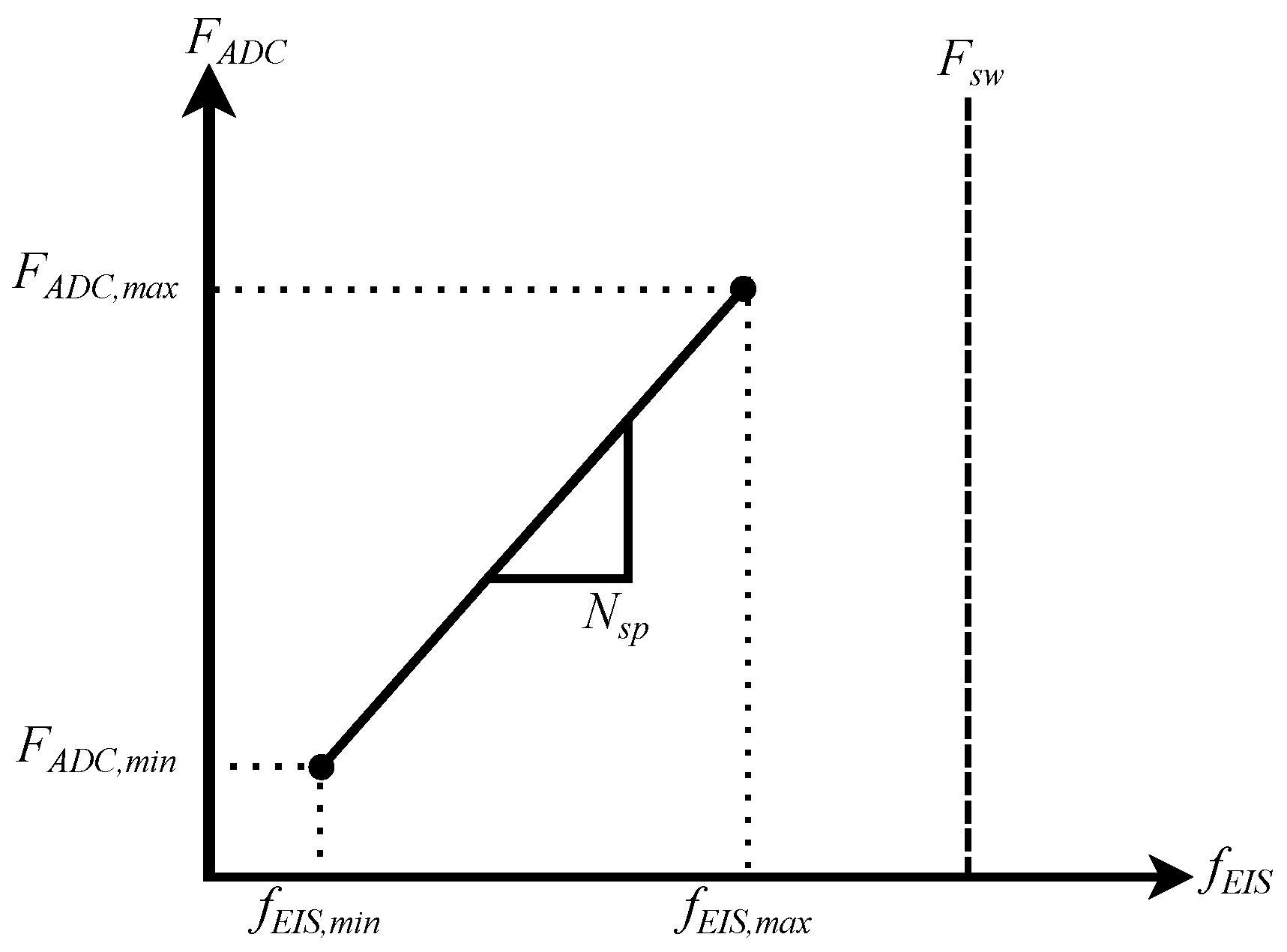
• First step: to define the number of samples $N_{FFT}$.
• Second step: to establish the $f_{EIS}$ range limited by the switching frequency $F_{sw}$, the ADC capabilities, and the samples per period $N_{sp}$.
• Third step: to define the number of periods $N_p$ to be acquired.
• Fourth step: using the previous results, to verify that the $f_{EIS}$ range, the $N_{sp}$, and the $N_p$ are within the ADC range.

As for the $N_{FFT}$ value, a large amount of data influences positively the quality of frequency analysis results but increases the memory requirements. The $N_{FFT}$ value should be in base-2 for an efficient signal processing. Indeed, in [37,38], the performance of the efficient calculation of the FFT with a different $N_{FFT}$ is described. The typical values of $N_{FFT}$ are 1024, 2048, 4096, and 8192, which correspond to the most common capacities found in different chips and values reported in studies available in the literature, e.g., in [37,38]. In order to analyse the effect of small, medium, and large $N_{FFT}$ values over the EIS method result, all these typical values were considered.

As for the perturbation frequency range $f_{EIS}$, three elements have to be kept into account: the switching frequency $F_{sw}$, the acquisition frequency range of the signals, which is limited by the ADC capabilities, and the number of samples per period $N_{sp}$, which must be chosen above a minimum value to have a correct representation of the analog signal.

The number of samples per period $N_{sp}$ has an impact on the frequency analysis. In theory, the Nyquist–Shannon sampling theorem indicates the minimum $N_{sp}$ value is 2 per period. However, in practical applications that value should be higher, so that the requirements concerning the memory capacity become more critical. In [39], an analysis about the impact of $N_{sp}$ value is presented. Typical values of $N_{sp}$, ranging from 8 until 512, were considered. The analysis was performed by considering the Texas Instruments ADS1274 24-bit analog–digital converter. It allows to configure the acquisition frequency in the range of $F_{ADC,max}$ = 144 kHz and $F_{ADC,min}$ = 0.039 kHz. Therefore, the maximum and minimum perturbation frequencies were calculated: $f_{EIS,max}=F_{ADC,max}/N_{sp}$ and $f_{EIS,min}=F_{ADC,min}/N_{sp}$, respectively. The calculation of $f_{EIS}$ in the mentioned different cases of $N_{sp}$ and $F_{ADC}$ is presented in

Table 5. Maximum and minimum perturbation frequency limited by ADC.

	FADC,max = 144 kHz	FADC,min = 0.039 kHz
Nsp	fEIS,max	fEIS,min
8	18,000	4.87
16	9000	2.43
32	4500	1.21
64	2250	0.60
128	1125	0.30
256	562.5	0.15
512	281.2	0.076

.

An acquisition frequency 144 kHz and $N_{sp}=8$ are a good choice to reach the EIS test close to switching frequency $F_{sw}$ = 20 kHz, but the precision of the impedance estimation must be studied.

On the other hand, the accuracy of frequency analysis depends also on the number $N_p$ of periods acquired for each signal, which has a direct relationship on the time needed to perform the entire acquisition, called hereafter the time window ($T_w$). Equation (7) reveals the relationship between $T_w$, the number of samples to do the FFT analysis $N_{FTT}$, and the ADC frequency $F_{ADC}$. The relationship $f_{EIS}=F_{ADC}/N_{sp}$ was used:

$$T_w=\frac{N_p}{f_{EIS}}=\frac{N_{FFT}}{F_{ADC}}$$

(7)

where $N_{FFT}=N_p{N}_{sp}$

The third step is to establish the number of periods of the signals $N_p=N_{FFT}/N_{sp}$. By considering the previously discussed set $N_{FFT}=\{1024,2048,4096,8192\}$,

Table 6. Number of periods $N_p$ and maximum time window $T_{w,max}$ for different $N_{FFT}$ and $N_{sp}$ with $F_{ADC,min}$.

	Nsp = 8	Nsp = 64	Nsp = 128
NFFT	Np			Tw,max [s]
1024	128	16	8	26.25
2048	256	32	16	52.51
4096	512	64	32	105.02
8192	1024	128	64	210.05

shows the $N_p$ required to perform the FFT analysis with different accuracy levels. Three values $N_{sp}=\{8,64,128\}$ were used. The $T_w$ required for the worst-case frequency in the EIS test, i.e., at low frequency, is also presented. At the lower ADC frequency and with the largest amount of data, the acquisition procedure takes 210.05 s.

The fourth step is to verify that the $f_{EIS}$ range is within the ADC range by using the constraints of $N_p$, $N_{sp}$, and $N_{FFT}$. Due to the wide range of possibilities of such parameters, an interception range was obtained. Figure 13 shows that the ADC range corresponds to a linear equation, where the slope is $N_{sp}$. Additionally, the $f_{EIS,max}$ must be kept below $F_{sw}$. The ADC range must be within the operating limits of the selected ADC.

Table 5 provides ranges of $f_{EIS}$ for different values of $N_{sp}$ and limited by $F_{ADC}$. Moreover, Table 6 provides the $N_p$ depending on the $N_{FFT}$ and $N_{sp}$ values. By using the relationship shown in Figure 13, and by choosing the values $N_{sp}=\{8,64,128\}$, the resulting $f_{EIS}$ ranges to be used were (4.87–18,000) Hz, (0.60–2250) Hz, and (0.30–1125) Hz, respectively. In order to keep in each experiment the same number of data, the range of $f_{EIS}$ = (10–1000) Hz was selected for the cases $N_{sp}=\{64,128\}$. With $N_{sp}=8$, the $f_{EIS,max}$ limit was the larger one, and thus an extended sweep-frequency experiment was possible. Therefore, for $N_{sp}=8$, $f_{EIS,max}$ is settled to 10,000 Hz. In all the experiments, ten values per decade are used for the estimation procedure. Additionally, in the experiment two perturbation amplitudes, 5%, and 10%, of the nominal duty cycle are tested. Therefore, a total of 24 experiments were done.

Table 7. Parameters and ranges of EIS experiments.

Parameters	Value or Range
Samples per period and $N_{FFT}$
$N_{sp}$	{8, 64, 128}
$N_{FFT}$	{1024, 2048, 4096, 8192}
Frequency range
$f_{EIS}$ range	$(10-10k)$ Hz for $N_{sp}=8$ $(10-1k)$ Hz for $N_{sp}=\{64,128\}$
$F_{ADC}$	$(80-8k)$ Hz for $N_{sp}=8$ $(640-64k)$ Hz for $N_{sp}=64$ $(1280-128k)$ Hz for $N_{sp}=128$
$F_{ADC}$ total range	{80 Hz to 128 kHz}

summarizes the main parameters of the experiments used in simulation with different $F_{ADC}$ values in terms of $N_{sp}$, $N_{FFT}$, and perturbation frequencies $f_{EIS}$ range.

5. Discussion

5.1. Analysis of Estimation Errors of C and ESR Indicators by Using the EIS Approach

The results obtained from using the proposed EIS method described in Section 4, and taking into account the previous hardware requirements, are shown in

Table 8. Percentage error estimating C and $ESR$ with $A_d=5\%$ of the nominal duty cycle.

${\mathit{N}}_{\mathit{F}\mathit{F}\mathit{T}}$		1024	2048	4096	8192
$N_p$		128	256	512	1024
$N_{sp}=8$	ESR	2.98	1.65	1.92	1.13
	C	5.13	9.18	10.18	10.04
$N_p$		16	32	64	128
$N_{sp}=64$	ESR	24.52	3.49	3.49	1.05
	C	30.31	0.18	0.50	5.18
$N_p$		8	16	32	64
$N_{sp}=128$	ESR	20.32	15.80	6.46	5.58
	C	26.40	19.09	10.68	10.36

and

Table 9. Percentage error estimating C and $ESR$ with $A_d=10\%$ of the nominal duty cycle.

${\mathit{N}}_{\mathit{F}\mathit{F}\mathit{T}}$		1024	2048	4096	8192
$N_p$		128	256	512	1024
$N_{sp}=8$	ESR	6.15	5.81	2.53	2.80
	C	9.77	9.24	6.39	7.60
$N_p$		16	32	64	128
$N_{sp}=64$	ESR	21.28	3.93	0.53	2.29
	C	19.86	3.99	0.37	2.39
$N_p$		8	16	32	64
$N_{sp}=128$	ESR	3.78	11.01	4.42	2.37
	C	2.32	11.72	3.88	0.11

. Table 8 shows capacitance and $ESR$ estimation errors for the selected values of $N_{FFT}$ and $N_p$, where the perturbation amplitude was 5%. For $N_{sp}=64$ with $N_{FFT}=2048$, the capacitance estimation error was less than 0.2%. For $N_{sp}=64$ with $N_{FFT}=8192$, the $ESR$ estimation error was less than 1.1%. The largest errors in the parameters estimation were obtained using the lower number of samples $N_{FFT}=1024$, in particular taking $N_{sp}=64$. It is worth noting that the better estimation of both parameters was not achieved by taking the largest amount of data $N_{FFT}=8192$, because of the influence of the perturbation amplitude, which is revealed in Table 9.

Table 9 shows the capacitance and the $ESR$ estimation errors when the perturbation amplitude was settled at 10% of the nominal duty cycle, which is in the limit of small-signal analysis. Unfortunately, it appeared to be too large for ensuring a stationary and stable converter operation. For $N_{sp}=8$, the estimation error decreased when more periods of signals were acquired. For $N_{sp}=64$ with $N_{FFT}=4096$, the error percentages were less than 0.6%, in contrast to the case of $N_{FFT}=1024$, where the errors were close to 20%. In the case of $N_{sp}=128$ with $N_{FFT}=8192$, capacitance and ESR estimation errors were less than 2.4% and 0.2%, respectively.

The ADC configuration of $N_p=64$, $N_{sp}=64$, and $N_{FFT}=4096$ exhibited the lower estimation error of both parameters, which was 0.6%. Moreover, the selected configuration spends lower computation time than cases with higher $N_p$ values. In terms of memory, the selected configuration requires a lower capacity store than the cases where $N_{FFT}=8192$ are used. However, the perturbation amplitude was 10%, which is in the limit of the small-signal analysis.

5.2. Analysis of Measurement Requirements

The bandwidth of sensors have to be in the frequency range of current and voltage signals to be acquired. Therefore, voltage and current sensors must have a time response ($t_r$) faster than the period of injected frequency, i.e., $t_r<1/f_{EIS,max}$. These values are fulfilled by commercial sensors such as the LEM LV25-P voltage transducer, which has a time response of $t_{r,voltage}=40$ μs [40]. In the case of the current sensor, the ACS37002 exhibited a time response of $t_{r,current}=1.1$ μs [41]. So, those kind of sensors keep the requirements of $t_{r,current}$ and $t_{r,voltage}$ lower than $1/f_{EIS,max}=100$ μs. Moreover, the conditioning stage of voltage and current signals must have high-pass filters to eliminate frequencies lower than the $f_{EIS,min}$. After, those signals are amplified to the input levels of the data-processing system.

5.3. Analysis of Signal Processors to Develop the FFT

Many applications are based on the FFT analysis, in which the processing signals’ capabilities of hardware define a part of its development. In fact, memory range and processor capacity are key features to select devices where FFT is executed. For example, in [38], Texas Instrument developed a system-on-chip, which includes FFTCs coprocessors dedicated to running an FFT algorithm; DSPs and ARMs cores to develop the other tasks required for a modern radar system. In that work, a high performance of the proposed FFTCs coprocessors was demonstrated by making a comparison among FFTCs and C66x DSP cores for developing a FFT algorithm. Features such as the capacity of operations and the signal-to-noise-ratio, in different cases of FFT sizes (up to 8192) were analyzed. However, the cost of the proposed system-on-chip board can avoid its massive commercial implementation for other applications.

Nevertheless, low-cost systems like the ARM-microcontroller STM32f427VGT6 and the BeagleBone development platform, equipped with an Arm Cortex-A8 processor, have seen significant growth in recent years. The former is able to generate the perturbation signal and develop the data processing. An FFT procedure up to 4096 samples, using the STM32f427VGT6, has been confirmed in [42]. Besides, its C programming availability allows the use of libraries to make the fit procedure and then to estimate the proposed indicators [43,44]. Meanwhile, some features like a Linux-based OS, processor speed, memory, as well as the availability of other resources on the board make the BeagleBone a more flexible solution in a wide-ranging applications. In [39], an experimental setup to model a fuel-cell by using an FFT analysis was presented by using a BeagleBone Black board. That system has a capacity to store up to twenty thousand samples for two different signals, using an FFT size up to 8192. Due to its low cost and its high-performance features, a ARM-microcontroller STM32f427VGT6 is considered to be used to develop the proposed EIS method for DC-link capacitors of fault-diagnosis.

5.4. Comparison of the Proposed EIS Technique with Online Diagnostic Methods Proposed in the Literature

Table 10. Implementation aspects of the methods proposed in literature.

Reference Number	Number and Type of Sensors	Signal Processor	Fundamental Strategy	Type of Processing Algorithm
[16]	Two current sensors and one voltage sensor, unspecified reference.	DSP, unspecified reference	Perturbing capacitor  voltage reference at 50 Hz	None. Estimation of C based on measurements and analytical expression.
[17]	Three current sensors LA-25 NP and one voltage sensor LV-25 NP.	DSP TMS320VC33	Perturbing AC current reference at 30 Hz	Estimation of ESR by RLS method
[18]	One current and one voltage sensors, unspecified reference.	Unspecified reference	Estimation of capacitor current and measuring voltage variation in zero state of transistor.	None. Estimation of C by analytical expression
[19]	Two current sensors LA-25P and one voltage sensor, unspecified reference.	DSP TMS320F2808	Extracted the second harmonic ripple of current, and voltage appeared in DC-link capacitor.	None. Estimation of Z by reconstructing capacitor current and measuring capacitor voltage
[20]	Two current sensors and one voltage sensor, unspecified reference.	DSP TMS320F2808	Estimation of current capacitor during switching period, and temperature estimation.	Estimate C and ESR, in a PoF model, by LMS and extended Kalman filter
Proposed method	One current sensor ACS37002 and one voltage sensor LV25-P.	ARM-microcontroller STM32f427VGT6	Perturbing PWM signal by sweep frequency	Estimation of C and ESR by Multifitting

presents a comparison among some recent online diagnostic methods available in the literature and the proposed EIS approach, by looking at the implementation aspects. The number and type of sensors, the signal processor technology, and the fundamental strategy and type of algorithm to process measurement data were selected as the most relevant features to compare. The estimation errors resulting by the application of the same methods were compared in Table 1 of the introduction. The only technique estimating both indicators C and ESR is the one in [20]. The estimation errors achieved by [20] were 2.14% and 0.19% for ESR and C indicators, respectively. Instead, the technique proposed in this study provided ESR and C estimation errors equal to 0.53% and 0.37%, respectively, thus improving the ESR estimation by 75.3%.

On the other hand, the determination of the capacitor current and voltage values, both RMS and ripple amplitudes at particular or different frequencies, to be used in analytical expressions or numerical algorithms, is the base of the different diagnostic methods in the literature. In [18,20], the capacitor voltage was measured; meanwhile, its current was reconstructed by using other measurements, this having an impact on the number of required sensors, as it is shown in Table 10. In the topology proposed in [18], the fact that the current capacitor was equal to the PV source current, when the input transistor of the converter was in the zero state, was exploited. Unfortunately, the measurement of the capacitor voltage in that zero state period is required, this being one of the main challenges of that technique, since the zero state period might be very short. In [20], the reconstruction of capacitor current is given by the AC side’s measured current and a particular relation among the current capacitor and the switching states. Meanwhile, the approach presented in [19] takes advantage of the fact that the DC-link experiment has a high harmonic component at a frequency that is the double that of the grid one. In that case, the capacitor voltage is directly acquired and the current capacitor and is reconstructed by measuring the grid side and PV source currents. The fundamental strategy of the methods proposed in [16,17] is to inject a perturbation signal. For the DC/DC converter presented in [16], a perturbation signal at 50 Hz was added to a reference signal of capacitor voltage, in a voltage control loop, which produces perturbed signals of currents and voltage in the capacitor. The capacitor voltage was directly measured, but the capacitor current was calculated by using the load and secondary DC-link currents; thus, three sensors were required. In the same way, a signal at 30 Hz was added in the AC-side current control loop of the on-grid system presented in [17]. Additionally, in that three-phase system, more than two sensors were required, because each line current has to be measured. In the last column of Table 10, the type of processing algorithm to determine ESR and C is highlighted. The diagnostic techniques proposed in [16,18,19] use analytical expressions, while [17,18,19,20] use algorithms, to determine ESR and C or only one of them for the DC-link capacitor. In [20], two processing algorithms were required. An extended Kalman filter allows to update a physics of failure (PoF) model, and a least mean square method allows to determine the C and ESR values. Meanwhile, in [17], only a recursive least square (RLS) method was used, but only ESR was determined. The technique proposed in this study, instead, employed a multifitting algorithm allowing to estimate both C and ESR. Contrary to the technique of [17], the proposed method was able to work without affecting the normal operation of the PV system, which operates with a varying PV input power and with an operating point that is periodically perturbed by the MPPT algorithm. The performance of the proposed diagnostic method is not affected by the normal operation of the PV system, such as the MPPT and the inverter controllers.

Finally, Table 10 allows to put into evidence that many techniques proposed in the literature use DSP platforms, such as [17,19,20], in which TMS320VC33 and TMS320F2808 boards have been employed, respectively. Meanwhile, the technique proposed in this study, which also have the lower estimation errors, requires $N_{FFT}=4096$ and $N_p=64$, which give better results than $N_{FFT}=8192$ and $N_p=128$ (see Table 9), can be implemented in a low-cost system, such as the ARM-microcontroller STM32f427VGT6 board.

6. Conclusions

This study proposed a diagnosis aging method of the DC-link capacitor in a single-phase grid-connected PV system. In the first stage of estimation of degradation indicators, the EIS approach was used to inject low-frequency signals in the PWM of the boost converter, avoiding turn-off of the converter or changing the operating point of the system. An FFT analysis was required to obtain the phase and magnitude impedance curves of the capacitor to be diagnosed. A multifitting algorithm based on simultaneous fitting of multiple non-linear curves with shared parameters allowed us to obtain mean square errors close to 1. An analysis of the ADC requirements demonstrated that a maximum acquiring frequency should be close to 128 kHz, which is provided by common commercial chips. A capacitor model of the two parameters capacitance and equivalent series resistance were adopted. In order to reach good accuracy in the estimation of those indicators of degradation, the number of samples per period and the periods should keep a trade-off. The developed experiments reveal that samples per period and period values higher than 32 and 64, respectively, meet errors in estimation lower than 3%. Additionally, the magnitude of perturbation must be in the range of small signals, but 10% of that magnitude concerning the operating point produces fewer errors in the estimation of C and $ESR$ than using 5% because the excitation of the system is lower. The second stage develops a comparison of estimated degradation indicator values that respect those nominal values. Because of the literature recommendation, a degradation of 80% of C and an increment of 200% in $ESR$ were set as thresholds. For implementing a FFT algorithm in a development system, two main technical aspects should be considered: system memory capacity to establish the maximum number of samples able to be stored and processed and computing capacity to execute the FFT analysis. A cost feature also determines a selection of processor signal, but a ARM-microcontroller STM32f427VGT6 is a promising solution for the proposed EIS method.

References

1. Qaedi, R.; Samet, H. Evaluation of Various Fault Detection Methods in non-Isolated Single Switch DC-DC Converters. In Proceedings of the 2018 IEEE International Conference on Environment and Electrical Engineering and 2018 IEEE Industrial and Commercial Power Systems Europe (EEEIC/I&CPS Europe), Palermo, Italy, 12–15 June 2018; pp. 1–5. [Google Scholar] [CrossRef]
2. Gupta, A.; Yadav, O.P.; DeVoto, D.; Major, J. A Review of Degradation Behavior and Modeling of Capacitors. In Proceedings of the ASME 2018 International Technical Conference and Exhibition on Packaging and Integration of Electronic and Photonic Microsystems, Taipei, Taiwan, 24–26 October 2018. [Google Scholar] [CrossRef] [Green Version]
3. Soliman, H.; Wang, H.; Blaabjerg, F. A Review of the Condition Monitoring of Capacitors in Power Electronic Converters. IEEE Trans. Ind. Appl. 2016, 52, 4976–4989. [Google Scholar] [CrossRef]
4. Wang, H.; Blaabjerg, F. Reliability of Capacitors for DC-Link Applications in Power Electronic Converters—An Overview. IEEE Trans. Ind. Appl. 2014, 50, 3569–3578. [Google Scholar] [CrossRef] [Green Version]
5. Jano, R.; Pitica, D. Accelerated ageing tests for predicting capacitor lifetimes. In Proceedings of the 2011 IEEE 17th International Symposium for Design and Technology in Electronic Packaging (SIITME), Timisoara, Romania, 20–23 October 2011; pp. 63–68. [Google Scholar] [CrossRef]
6. Zhao, Z.; Davari, P.; Lu, W.; Wang, H.; Blaabjerg, F. An Overview of Condition Monitoring Techniques for Capacitors in DC-Link Applications. IEEE Trans. Power Electron. 2021, 36, 3692–3716. [Google Scholar] [CrossRef]
7. Lipnicki, P.; Lewandowski, D.; Orkisz, M.; Tresch, A. The effect of change in DC link series resistance on the AC/AC converter operation: Power converters embedded diagnostics. In Proceedings of the 2013 IEEE 1st International Conference on Condition Assessment Techniques in Electrical Systems (CATCON), Kolkata, India, 6–8 December 2013; pp. 122–127. [Google Scholar] [CrossRef]
8. Wang, H.; Nielsen, D.A.; Blaabjerg, F. Degradation testing and failure analysis of DC film capacitors under high humidity conditions. Microelectron. Reliab. 2015, 55, 2007–2011. [Google Scholar] [CrossRef]
9. Ren, L.; Gong, C.; Zhao, Y. An Online ESR Estimation Method for Output Capacitor of Boost Converter. IEEE Trans. Power Electron. 2019, 34, 10153–10165. [Google Scholar] [CrossRef]
10. Farjah, E.; Givi, H.; Ghanbari, T. Application of an Efficient Rogowski Coil Sensor for Switch Fault Diagnosis and Capacitor ESR Monitoring in Nonisolated Single-Switch DC–DC Converters. IEEE Trans. Power Electron. 2017, 32, 1442–1456. [Google Scholar] [CrossRef]
11. Kai, Y.; Wenbin, H.; Weijie, T.; Jianguo, L.; Jingcheng, C. A novel online ESR and C identification method for output capacitor of buck converter. In Proceedings of the 2014 IEEE Energy Conversion Congress and Exposition (ECCE), Pittsburgh, PA, USA, 14–18 September 2014; Volume 2, pp. 3476–3482. [Google Scholar] [CrossRef]
12. Yao, K.; Tang, W.; Bi, X.; Lyu, J. An Online Monitoring Scheme of DC-Link Capacitor’s ESR and C for a Boost PFC Converter. IEEE Trans. Power Electron. 2016, 31, 5944–5951. [Google Scholar] [CrossRef]
13. Sun, Q.; Wang, Y.; Jiang, Y.; Wu, Y. On-line component-level soft fault diagnostics for power converters. In Proceedings of the 2016 Prognostics and System Health Management Conference (PHM-Chengdu), Chengdu, China, 19–21 October 2016; pp. 1–5. [Google Scholar] [CrossRef]
14. Meng, J.; Chen, E.X.; Ge, S.J. Online E-Cap Condition Monitoring Method Based on State Observer. In Proceedings of the 2018 IEEE International Power Electronics and Application Conference and Exposition (PEAC), Shenzhen, China, 4–7 November 2018; pp. 1–6. [Google Scholar] [CrossRef]
15. Ertasgin, G.; Whaley, D.M.; Ertugrul, N.; Soong, W.L. Analysis of DC Link Energy Storage for Single-Phase Grid-Connected PV Inverters. Electronics 2019, 8, 601. [Google Scholar] [CrossRef] [Green Version]
16. Hannonen, J.; Honkanen, J.; Ström, J.P.; Korhonen, J.; Silventoinen, P.; Räisänen, S. Capacitance measurement method using sinusoidal voltage injection in isolating phase-shifted full-bridge DC–DC converter output stage. IET Power Electron. 2016, 9, 2543–2550. [Google Scholar] [CrossRef]
17. Pu, X.S.; Nguyen, T.H.; Lee, D.C.; Lee, K.B.; Kim, J.M. Fault Diagnosis of DC-Link Capacitors in Three-Phase AC/DC PWM Converters by Online Estimation of Equivalent Series Resistance. IEEE Trans. Ind. Electron. 2013, 60, 4118–4127. [Google Scholar] [CrossRef]
18. Agarwal, N.; Ahmad, M.W.; Anand, S. Condition monitoring of dc-link capacitor utilizing zero state of solar PV H5 inverter. In Proceedings of the 2016 10th International Conference on Compatibility, Power Electronics and Power Engineering (CPE-POWERENG), Bydgoszcz, Poland, 29 June–1 July 2016; pp. 174–179. [Google Scholar] [CrossRef]
19. Arya, A.; Ahmad, M.W.; Agarwal, N.; Anand, S. Capacitor impedance estimation utilizing dc-link voltage oscillations in single phase inverter. IET Power Electron. 2017, 10, 1046–1053. [Google Scholar] [CrossRef]
20. Gupta, Y.; Ahmad, M.W.; Narale, S.; Anand, S. Health Estimation of Individual Capacitors in a Bank With Reduced Sensor Requirements. IEEE Trans. Ind. Electron. 2019, 66, 7250–7259. [Google Scholar] [CrossRef]
21. Miao, W.; Lam, K.H.; Pong, P.W.T. Online Monitoring of Aluminum Electrolytic Capacitors in Photovoltaic Systems by Magnetoresistive Sensors. IEEE Sens. J. 2020, 20, 767–777. [Google Scholar] [CrossRef]
22. Ahmad, M.W.; Agarwal, N.; Kumar, P.N.; Anand, S. Low-Frequency Impedance Monitoring and Corresponding Failure Criteria for Aluminum Electrolytic Capacitors. IEEE Trans. Ind. Electron. 2017, 64, 5657–5666. [Google Scholar] [CrossRef]
23. Aeloiza, E.; Jang-Hwan, K.; Enjeti, P.; Ruminot, P. A Real Time Method to Estimate Electrolytic Capacitor Condition in PWM Adjustable Speed Drives and Uninterruptible Power Supplies. In Proceedings of the IEEE 36th Conference on Power Electronics Specialists, Dresden, Germany, 16 June 2005; pp. 2867–2872. [Google Scholar] [CrossRef]
24. Wang, G.; Guan, Y.; Zhang, J.; Wu, L.; Zheng, X.; Pan, W. ESR estimation method for DC-DC converters based on improved EMD algorithm. In Proceedings of the IEEE 2012 Prognostics and System Health Management Conference (PHM-2012 Beijing), Beijing, China, 23–25 May 2012; pp. 1–6. [Google Scholar] [CrossRef]
25. Yu, Y.; Zhou, T.; Zhu, M.; Xu, D. Fault Diagnosis and Life Prediction of DC-link Aluminum Electrolytic Capacitors Used in Three-phase AC/DC/AC Converters. In Proceedings of the 2012 Second International Conference on Instrumentation, Measurement, Computer, Communication and Control, Harbin, China, 8–10 December 2012; pp. 825–830. [Google Scholar] [CrossRef]
26. Dubilier, C. Aluminum Electrolytic Capacitor Application Guide; Technical Report 864; Cornell Dubilier: South Plainfield, NJ, USA, 2011. [Google Scholar]
27. Czarkowski, D. DC-DC Converters. In Power Electronics Handbook, 4th ed.; Rashid, M.H., Ed.; Elsevier: Amsterdam, The Netherlands, 2018; Chapter DC-DC Conv; pp. 275–288. [Google Scholar] [CrossRef]
28. Abdennadher, K.; Venet, P.; Rojat, G.; Retif, J.M.; Rosset, C. A Real-Time Predictive-Maintenance System of Aluminum Electrolytic Capacitors Used in Uninterrupted Power Supplies. IEEE Trans. Ind. Appl. 2010, 46, 1644–1652. [Google Scholar] [CrossRef] [Green Version]
29. Vogelsberger, M.A.; Wiesinger, T.; Ertl, H. Life-Cycle Monitoring and Voltage-Managing Unit for DC-Link Electrolytic Capacitors in PWM Converters. IEEE Trans. Power Electron. 2011, 26, 493–503. [Google Scholar] [CrossRef]
30. Venet, P.; Perisse, F.; El-Husseini, M.; Rojat, G. Realization of a smart electrolytic capacitor circuit. IEEE Ind. Appl. Mag. 2002, 8, 16–20. [Google Scholar] [CrossRef]
31. Lasia, A. Electrochemical Impedance Spectroscopy and its Applications; Springer: New York, NY, USA, 2014. [Google Scholar] [CrossRef]
32. Varnosfaderani, M.A.; Strickland, D. Online Electrochemical Impedance Spectroscopy (EIS) estimation of a solar panel. Vacuum 2017, 139, 185–195. [Google Scholar] [CrossRef] [Green Version]
33. Femia, N.; Petrone, G.; Spagnuolo, G.; Vitelli, M. Optimization of Perturb and Observe Maximum Power Point Tracking Method. IEEE Trans. Power Electron. 2005, 20, 963–973. [Google Scholar] [CrossRef]
34. Abo-Khalil, A.; Lee, D.-C. DC-Link Capacitance Estimation in AC/DC/AC PWM Converters Using Voltage Injection. IEEE Trans. Ind. Appl. 2008, 44, 1631–1637. [Google Scholar] [CrossRef]
35. Chen. Multiple Curve Fitting with Common Parameters Using NLINFIT. Available online: https://www.mathworks.com/matlab-central/fileexchange/40613-multiple-curve-fitting-with-common-parameters-using-nlinfit (accessed on 7 July 2020).
36. United Chemi-Con, I. U36D Series Capacitor. Available online: https://www.micro-semiconductor.com/datasheet/de-E36D750HPN682QA79M.pdf (accessed on 7 October 2020).
37. Texas Instruments. Using DSPLIB FFT Implementation for Real Input and Without Data Scaling; Technical Report; Texas Instruments: Dallas, TX, USA, 2019. [Google Scholar]
38. Roh, J.C.; Aridhi, S. Optimizing Modern Radar Systems Using Low-Latency, High-Performance FFT Coprocessors; Texas Instruments: Dallas, TX, USA, 2016. [Google Scholar]
39. Petrone, G.; Zamboni, W.; Spagnuolo, G.; Dessi, R. EIS Method for the On-Board Evaluation of the Fuel Cell Impedance. In Proceedings of the 2018 IEEE 4th International Forum on Research and Technology for Society and Industry (RTSI), Palermo, Italy, 10–13 September 2018; pp. 1–6. [Google Scholar] [CrossRef]
40. LEM International SA. Voltage Transducer LV 25-P. Available online: https://www.lem.com/en/lv-25p (accessed on 5 February 2019).
41. Allegro MicroSystems. ACS37002 High Accuracy Current Sensor. Available online: https://www.allegromicro.com/en/product-s/sense/current-sensor-ics/zero-to-fifty-amp-integrated-conductor-sensor-ics/acs37002 (accessed on 2 October 2021).
42. STMicroelectronics. Library 62- Fast Fourier Transform (FFT) for STM32F4xx. Available online: www.ST.com (accessed on 2 October 2021).
43. Silicon Labs. CMSIS DSP Software Library. Available online: https://docs.silabs.com/cmsis/latest/dsp/api-index (accessed on 2 October 2021).
44. STMicroelectronics. Digital Signal Processing for STM32 Microcontrollers Using CMSIS. Available online: https://www.st.com/co-ntent/ccc/resource/technical/document/application_note/group0/c1/ee/18/7a/f9/45/45/3b/DM00273990/files/DM002739-90.pdf/jcr:content/translations/en.DM00273990.pdf (accessed on 2 October 2021).
Figure 1. Impedance characteristics of a degraded and non-degraded capacitor.
Energies 14 06754 g001
Figure 2. Models of aluminum electrolytic capacitors. (a) Model 1 [24]. (b) Model 2 [25]. (c) Model 3 [4].
Energies 14 06754 g002
Figure 3. A simplified equivalent model of capacitors [24].
Energies 14 06754 g003
Figure 4. Flowchart of the proposed diagnosis method.
Energies 14 06754 g004
Figure 5. Grid-connected single-phase PV system.
Energies 14 06754 g005
Figure 6. Feedforward and cascaded control of inverter.
Energies 14 06754 g006
Figure 7. Basic schemes of PLL and dq transform.
Energies 14 06754 g007
Figure 8. Output voltage of boost converter, duty-cycle, PV power, and irradiance.
Energies 14 06754 g008
Figure 9. Impedance of DC-link capacitor by using the EIS approach in different operating conditions.
Energies 14 06754 g009
Figure 10. Multiple curve-fitting for magnitude and phase with MPPT OFF at 400 W/m2. (a) Magnitude. (b) Phase.
Energies 14 06754 g010
Figure 11. Multiple curve-fitting for magnitude and phase with MPPT ON at 400 W/m 2 . (a) Magnitude. (b) Phase.
Energies 14 06754 g011
Figure 12. Multiple curve-fitting for magnitude and phase with MPPT ON at 750 W/m 2 . (a) Magnitude. (b) Phase.
Energies 14 06754 g012
Figure 13. Interrelation of the different frequencies.
Energies 14 06754 g013