Abstract
Having a photovoltaic (PV) system raises the question of whether it runs as expected. Measuring its energy yield takes a long time and the result still contains uncertainties from varying weather conditions and possible shading of the modules. Here, a free software PVcheck to measure the peak power of the system is announced, using the power data of a single sunny day. The software loads a data file of the generated power as a function of time from this day. This data file is provided by typical inverters. The software then simulates this power curve using known parameters like angle and location of the PV system. The assumed peak power of the simulation can then be adjusted so that the simulated curve matches the measured one. The software runs under Microsoft Windows™ and makes use of the free library pvlib python. The simulation can be refined by importing weather data like temperature, wind speed, and insolation. Furthermore, curves describing the nominal module efficiency as a function of the illumination intensity as well as the power-dependent inverter efficiency can be included in the simulation. First results reveal a good agreement of the simulation with experimental data. The software can be used to detect strong problems in PV systems after installation and to monitor their long-time operation.
1. Introduction
The amount of annual PV installations worldwide reached more than 135 GWp in 2020 [1], while the total amount of PV power capacity grew by about 29% yearly during the last decade [2]. It is important to be able to check whether a new installation is working as expected. Furthermore, monitoring system efficiency over time is necessary to detect and remedy possible PV system problems.
Comparing the energy yield of the PV system with the predicted value is a possibility, but requires an extended period of time, while the result continues to suffer from weather variations. Online databases can help to calculate the yield of a PV system. The free online service PVGIS [3] can give estimated hourly power production based on weather databases, but no actual data from recent years was available for many countries at the time of writing this paper. It mainly provides an estimated (yearly or monthly) yield of a PV system whose parameters can be given as an input. The PVWatts Calculator by the National Renewable Energy Laboratory also calculates the expected energy yield for a given month or the full year as a free service [4]. In addition, there are commercial software packages that mainly calculate typical energy yields for an average month or year. In all of these cases, measurement data for a long period of time is needed for a good estimate if the PV system in question is working as expected.
The power of a PV system is mainly dependent on its peak power (as defined under standard test conditions), the irradiation hitting its surface, the module temperature, and the efficiency of the inverter. There exist models for the calculation of the clear sky solar radiation incident on an inclined surface [5,6,7], as well as of the solar cell temperature [8].
The aim of this paper is to announce a software to check if a PV system is running as expected and to demonstrate typical results and limitations. The software mainly needs the power data from a sunny day and a few system parameters, as well as air temperature and wind speed. It does not do any PV yield prediction [9]. Instead, it “measures” the peak power of a PV system by fitting the simulated power curve for a day with clear sky to the measured power curve, with the peak power as the fit parameter. The difference to yield predictions is that the result is obtained with data from one sunny day and that the influence of shading (for instance from trees or clouds) is excluded.
The nominal peak power of a PV module (in Watt-peak, Wp) is given for standard test conditions from its data sheet, together with data on its lowlight behavior, as well as its temperature dependency. A factor for the inverter efficiency (from its data sheet) has to be added to get the nominal PV system peak power (excluding minor losses from cables, etc.).
The interesting question is if an existing PV system matches the expectations from its data sheets and how the peak power degrades over its lifetime. Larger PV systems can have sensors logging produced power over time as well as irradiation, air temperature and maybe wind speed. In this way, the influence of the weather can be eliminated from the power data and the efficiency of the system can be monitored. The aim of the announced software is to add such possibilities to even smaller residential systems that only provide logging data for produced power over time and do not have expensive weather sensors.
The solution proposed here is to make use of the well-developed free software library pvlib python [10] in combination with a graphical user interface (GUI) written for Microsoft Windows™, in combination with precise data from professional weather stations that exist in most countries. The main goal is to make the simulation models of pvlib python accessible via the GUI to people without python programming knowledge. The software PVcheck can be used freely from its website [11].
Test measurements show that simulated and measured power curves for a sunny day are in good agreement and result in reasonable values of the peak power of the system.
2. Method
The term “PV system peak power” is used here as the power that the PV system would deliver under standard test conditions (STC)—that is, illumination with 1000 W/m² light intensity with the atmospheric mass 1.5 (AM1.5) spectrum perpendicular to the surface of the PV modules, and 25 °C module temperature. Since a real PV system practically never operates under STC, calculations are necessary to take different illumination intensities, angles, and temperatures into account.
This method is based on the measurement of the system power as a function of time for a single sunny day. Many inverters have inbuilt loggers for produced system power over time, which can be exported as an ASCII file. PVcheck can import such files even in varying formats. An acceptable file may contain some header lines, which will be automatically identified and ignored, followed by lines with measurement data. Each data line must contain a time (and optionally a date), as well as one or several measured values separated by commas, spaces, etc. A block of lines with the same number of values is considered the usable body of the file.
The software then simulates this power curve with the system peak power as the fit parameter and displays the measured and the simulated power curve in the same diagram. For the simulation, the following parameters are needed:
- Position of the PV system (latitude, longitude, and altitude)
- Angle of the system (azimuth and tilt); all modules must have the same angle
- Time-zone, and whether a daylight-saving hour is added in summer
- Air temperature (constant or time-dependent)
- Wind speed (constant or time-dependent)
- PV system type (e.g., glass/polymer open rack)
- PV temperature coefficient (power change per temperature change)
- Albedo (ground reflection)
- Inverter efficiency (constant or power dependent)
Optionally, the module lowlight behavior from its datasheet can be added as a curve giving its relative efficiency as a function of the relative illumination intensity between zero and 1000 W/m². Additionally, the temperature coefficient of the PV modules should be found in its data sheet. Solar modules based on crystalline silicon solar cells have typical values around −0.4%/K. During the day, the air temperature normally changes significantly, and the modules also heat up under insolation. Pvlib python provides a model for calculating the temperature of the solar cells from the actual insolation, air temperature, wind speed and PV system type [8,12]. To get reasonable results, time-dependent air temperature and wind speed data is decisive—this data should be imported from nearby weather stations.
Since irradiation data might not always be available, PVlib’s clearsky model is used, which calculates the irradiation components of a clear blue sky. The Linke turbidity coefficient [13] as a function of the geographical position on earth and the time of the year is imported from a database that comes with pvlib python. Using this database, combined with a model from Ineichen and Perez, the clear sky irradiation is calculated in terms of diffuse normal irradiation (DNI), global horizontal irradiation (GHI) and diffuse horizontal irradiation (DHI) [6].
The precision of these irradiation values can be improved with measured GHI data from a nearby weather station, if available. In this case, the simulated PV power is factor-corrected with the quotient of the measured GHI and the simulated GHI.
The software PVcheck calculates the simulated PV power for exactly the same points in time as measured by the inverter. If the inverter exports average power values over the time intervals and not actual values, it is important that these time intervals are sufficiently small—typically a few minutes. Otherwise, the inverter data will be lagging behind the simulated data. The error from too large time intervals in power data is approximately given by half of the value changing over the interval. (In a typical case, this error is about 1% in the interval 11h until 12h, if only one-hour steps would have been available). In the test scenario reported here, the measured GHI data was used from a weather station with only a one-hour time resolution, where each GHI value was the averaged value over the last hour. Calculating a correction factor between these GHI values and the simulated GHI values produced errors due to the lag in the measured values. In that case, the simulated GHI values could also be averaged over the same time intervals as the measured ones.
After importing the measured PV power as a function of time as obtained from the inverter, the simulated power curve is adjusted manually to the measured power curve by modifying the system peak power of the simulation. When comparing both power curves for that day, periods of shading and even short time periods with clouds are identified by eye, so that the overall fitting of the correct system peak power is not significantly disturbed. The outcome of this procedure is the actual system peak power.
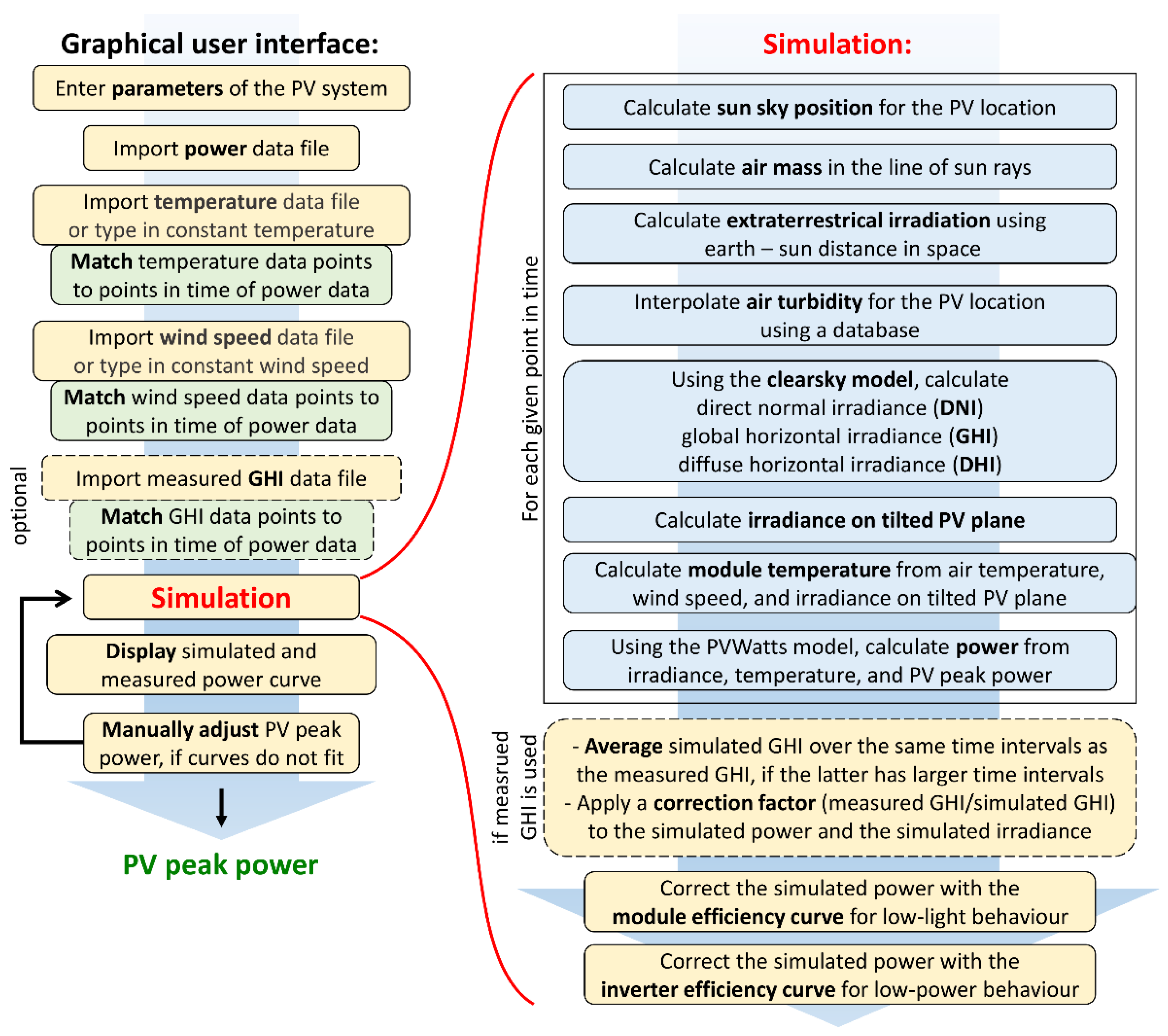
A simplified working scheme of PV check is depicted in Figure 1. The software is based on two programs running at the same time. The graphical user interface that was programmed using pascal (PVcheck.exe) is started first. This automatically loads the second program (PVlib.exe), based on python code, which is running in the background. Data transfer between the two programs is done via ASCII files.

Figure 1.
Flow diagram of PVcheck version 0.1. Pascal program parts are shown in orange and green boxes. “Matching” of temperature data points means that temperatures are only taken for the same points in time where imported power data is available. This is normally done by interpolation from the imported temperature data file. Matching of wind speed and GHI is done analogously. Python program parts using pvlib are shown in blue boxes and are enframed. Module and inverter efficiency curves are parts of the parameters of the system that have to be loaded in the beginning.
To test the software, a PV installation was evaluated that consisted of 45 multicrystalline modules with a nominal peak power of 12.8 kW located in Karlstad, Sweden. The inverter was a Sunny Tripower 10000TL from SMA. It limited the power to 10 kW to allow a cheap grid connection tariff with a nearly negligible energy yield. The system had three strings with 15 modules each—two of them connected in parallel. The modules were mounted in the summer of 2018 on a roof with an air gap of a few centimeters between the modules and the underlying concrete tiles. Such geometry is presumably best described by the “glass-polymer, open rack” setting of pvlib python. The system went into operation in January 2019 and is referred to as “PV system A” later in the text. Temperature and wind speed data came from a nearby airport (about 12 km away), as well as GHI data from another weather station (about 7 km away). Additionally, the in-plane irradiation was measured at the PV system using a calibrated detector (type Si-RS485TC-T-Tm-MB from Ingenieurbüro Mencke & Tegtmeyer GmbH, 31789 Hameln, Germany). This radiation detector consisted of a multicrystalline solar cell with an attached temperature sensor that was used to correct the irradiation measurement. Its nominal precision was 2.5% plus 5 W/m², which sums up to about 3% in this case. Additionally, the detector contains another temperature sensor that was glued to the back sheet of one the PV modules.
3. Results
3.1. Temperature Calculation
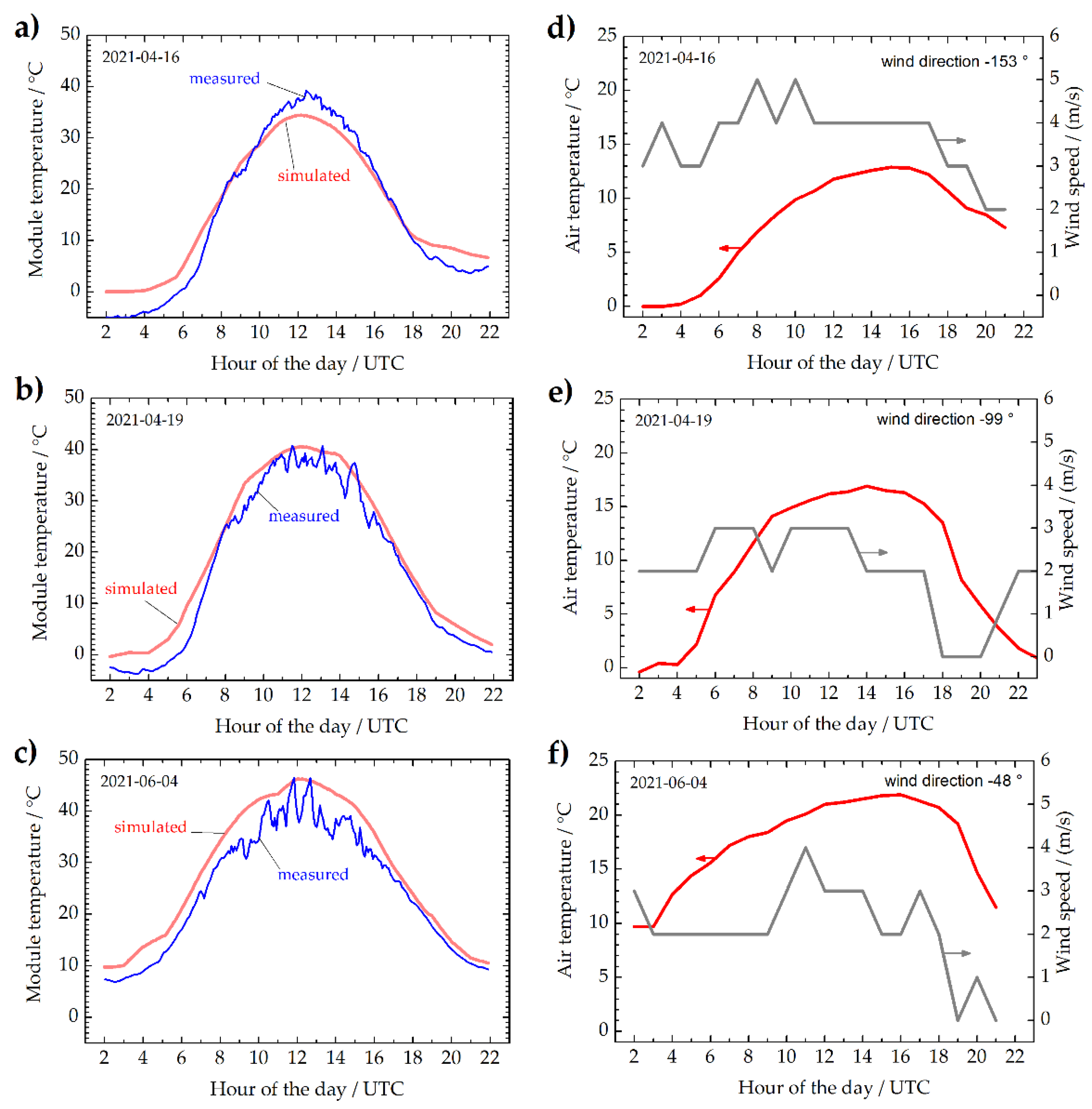
The results in Section 3.1, Section 3.2, and Section 3.3 were done using PVcheck, version 0.1. Using the test PV system, the simulated module temperatures (as calculated from measured air temperatures, wind speeds and the module type) were compared to the measured temperatures. Figure 2 shows the measured and simulated module temperatures for three sunny days. Both curves deviate by about 5 °C from each other around noon. In (a), the measured temperature was a bit higher than the simulated one. On this day, the wind speed was around 4 m/s during noon, but coming from behind the roof so that the PV system was in wind shadow. This probably led to a higher measured temperature. In (b), both temperature curves match better during noon. The wind blew nearly parallel to the surface of the modules with a little shaded component from behind. The nearly 90 ° relative wind direction represents an average case, where we here see the best correlation between simulated and measured temperature. In (c), the measured temperature was lower than the simulated one, possibly because of the stronger cooling effect of the wind which blew more towards the front of the modules. These results show an acceptable agreement between measurement and simulation. However, the wind direction could lead to a certain deviation. Temperature deviations of 5 °C typically correspond to about 2% inaccuracy of the calculated peak power of the system.
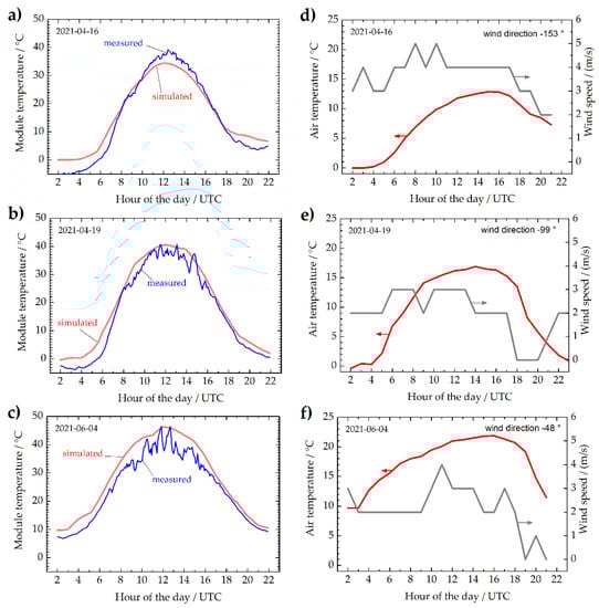
Figure 2.
Left column (a–c): Simulated and measured module temperatures on three different days (date in the upper left corner). Right column (d–f): Air temperature, wind speed, and average wind direction angle relative to the azimuth of the PV modules between 9 h and 15 h UTC on corresponding days.
3.2. Radiation Calculation
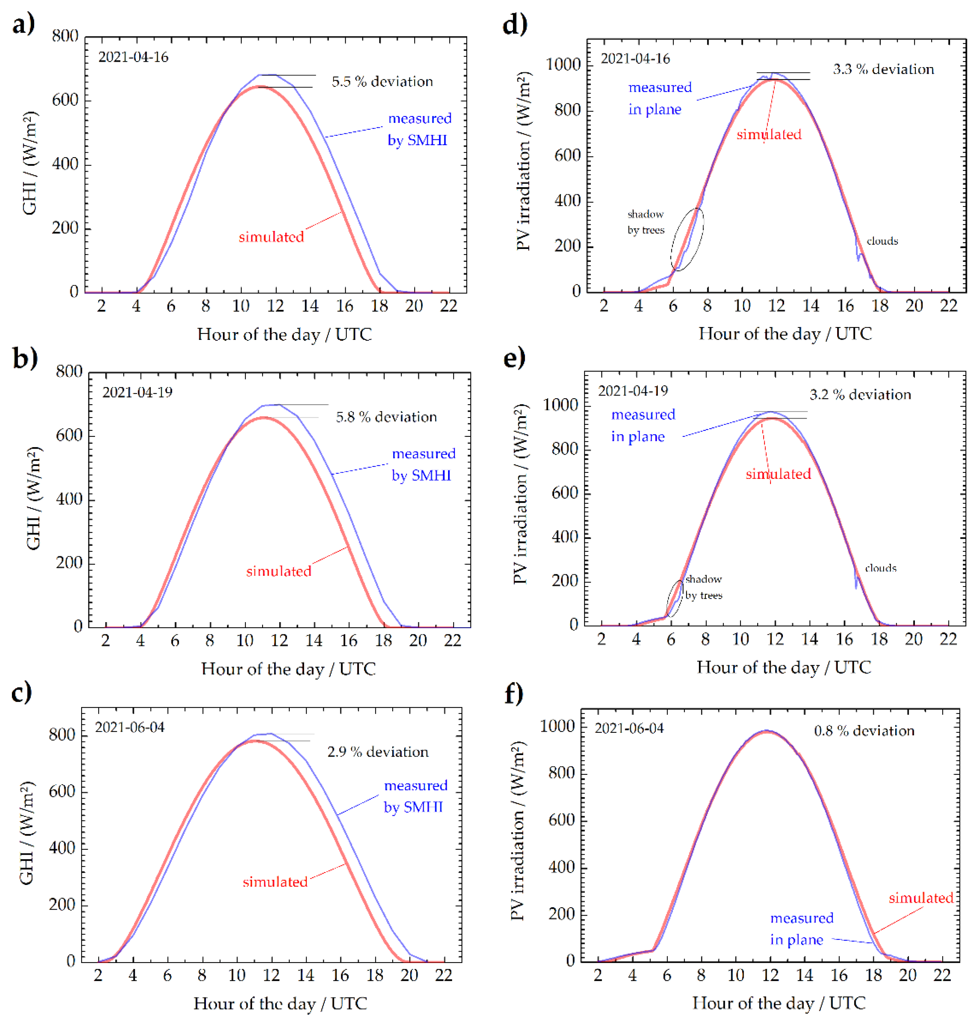
A comparison of simulated and measured irradiation curves is shown in Figure 3. The left column reveals measurements of the Swedish weather service SMHI in red, as can be downloaded from their website [14]. The data are GHI values that were averaged over all the previous hours. Since the simulation shows actual (non-averaged) values every 5 min, the values from SMHI lagged behind the simulated ones. This problem can be handled by also averaging the simulated values over full hours, which leads to two curves that deviate by a nearly constant factor (not shown here). The peak values of the measurements shown here were 2.9% to 5.8% larger than the ones of the simulation from the clearsky model.
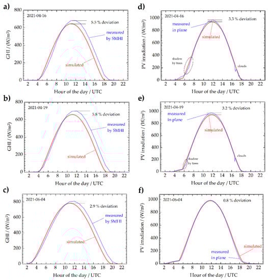
Figure 3.
Left column (a–c): Simulated and measured global horizontal irradiation (GHI) on three different days (date in the upper left corner). The measurement was done by a local weather station (Sveriges meteorologiska och hydrologiska institut, SMHI). Right column (d–f): Simulated and measured irradiation on corresponding days in the plane of the PV modules. The measurement was done using the above-named calibrated detector mounted directly near the PV modules. The simulations were done without shallow angle reflection correction (see Section 3.4).
The right column in Figure 3 shows the simulated and measured irradiation in the plane of the PV test system using the above-named radiation detector. This measurement best reflects the optical properties of the surroundings of the PV system (ground reflection and diffuse skylight shading from surrounding objects). Furthermore, the detector had a similar spectral response to the PV modules.
3.3. Simulated PV System Power
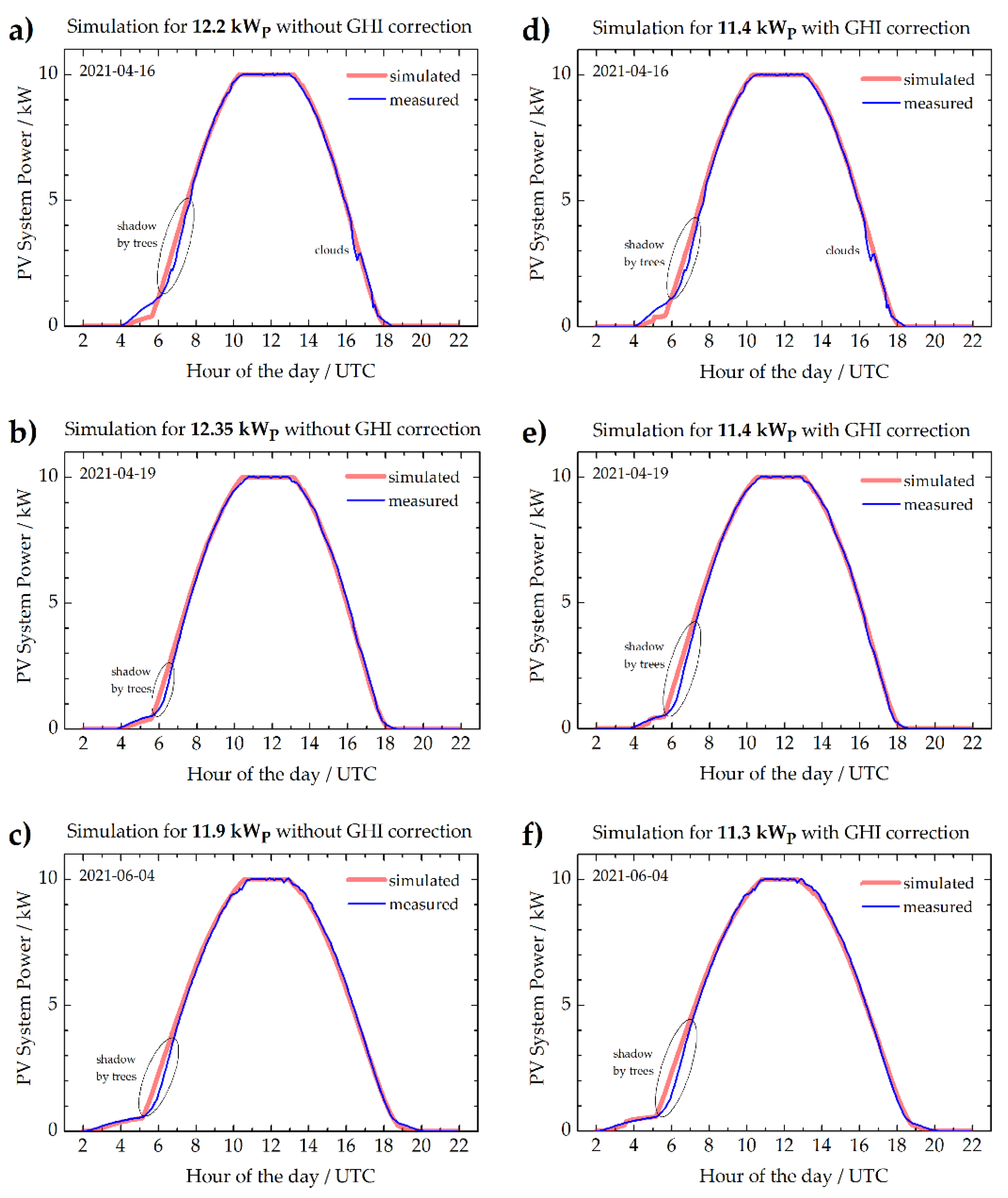
Figure 4 shows the simulated power compared to the power measured over three sunny days without incident angle modifier. For every day, a nominal power of the PV system was chosen which fit the measurement. The simulation used temperature and wind speed during these days as input data. In a first attempt, the irradiation was simulated using the clearsky model of pvlib python (Figure 4a–c). This led to a system peak power of 12.2, 12.35, and 11.9 kWp, as best fit of the simulation to the measured system power. Then, a correction factor (measured GHI/simulated GHI) was applied to the simulated system power before determining the best fitting system peak power (Figure 4d–f). On average, the system peak power was found to be 12.15 kW without using a GHI correction and 11.4 kW, including measured GHI data. This means that the correction with measured GHI data reduced the obtained system peak power of that system by 6.9%. Using the GHI correction also minimized the scatter between the three days. However, this may overestimate the diffuse light at the PV system if surrounded by other buildings.
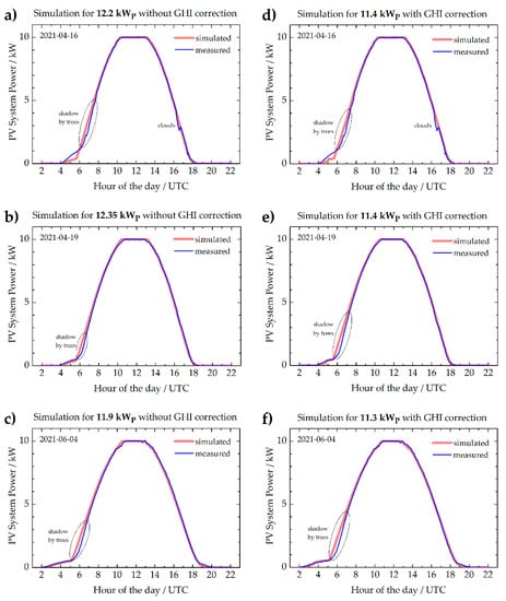
Figure 4.
Left column (a–c): Simulated and measured system power on three different days. The simulated curves using measured temperatures and wind speed, but without using measured GHI data, were fitted to the measured curves by adjusting the system peak power value to 12.2, 12.35, and 11.9 kWp. Right column (d–f): Simulated and measured system power on corresponding days, using temperature, wind speed, and measured GHI data by adjusting the system peak power value to 11.4 and 11.3 kWp. All power values were limited to 10 kW, which is the maximum inverter power. The simulations were done without shallow angle reflection correction (see Section 3.3).
3.4. Incident Angle Modifier
Light that hits PV modules with more shallow angles is reflected more strongly. This effect was included as an option in the simulation from PVcheck version 0.2 for direct, diffuse sky light, and diffuse light reflected from the ground using the incident angle modifier (IAM) from the analytical model from Martin and Ruiz [15,16]. For system A and the date 2021-04-16, the IAM reduced the radiation reaching the PV cells by 0.8% at the time of maximum power (approximately noon) and around 2% 3 hours earlier. This resulted in an increase in the determined peak power by about 1%. This effect is included in the following chapter.
3.5. Test of Different PV Systems
Typical results obtained with PVcheck are shown in Table 1 and Table 2 for five residential roof-top PV systems in Karlstad, Sweden. System A is the one already presented in the previous chapters, but now including a correction by the incident angle modifier.

Table 1.
Peak power values determined with PVcheck for five different PV systems and three sunny days each. The calculations include a correction by the incident angle modifier for direct and diffuse light. The numbers are furthermore corrected for inverter efficiency and module lowlight behaviour to show the peak power of the modules. Electrical cable losses are neglected. Part (a) shows results obtained with the Ineichen clearsky model only (without GHI correction). Part (b) includes a correction factor (measured GHI/simulated clearsky GHI) for the simulated irradiation. The nominal peak power is the given module power at standard test conditions from the datasheets, multiplied by the number of modules. For each system, the maximum allowed degradation from the datasheets is given on the right.
Table 2.
Determined peak power divided by the expected peak power of the five PV systems for three sunny days each. The expected peak power was taken as the nominal peak power that was reduced by the maximal nominal degradation over time from installation to the measurement; 100% means that the system runs as expected if the maximal allowed degradation has happened. Weather data was taken from the stations named in Section 2.
4. Discussion
The simulated cell temperatures typically deviated from the measured module temperatures by 5%, leading to an inaccuracy of about 2% in the simulated power values for typical modules based on crystalline silicon. These deviations can eventually be reduced if only days with wind directions parallel to the modules or days with low wind speeds are used.
Using the Ineichen clearsky model of pvlib python, the simulated irradiation on the tilted PV plane was somewhat lower than the measured one. The Ineichen model proved to be among the most precise [17], but still tended to underestimate the radiation during noon as well as during the first nine months of the year. A test over several locations in the USA resulted in average monthly errors between 0 and −40 W/m² in April. In general, the precision of the Ineichen model used is about 2%.
A comparison of the irradiation measurement in-plane with the modules of PV system A is shown in Figure 3d–f. The deviation to the Ineichen simulation without IAM is a little over 3% in April and 0.8% in June. This result is in agreement with the detector accuracy of 3% and the assumed Ineichen model accuracy of 2%. In agreement with [17], we saw a small underestimation of the irradiation by the Ineichen model.
If the in-plane measurement systematically gives larger values than the simulation, the lower deviation in June sticks out. One reason could be soiling due to pollen from pine trees, which typically produces a yellowish color deposit on the investigated PV modules at that time of the year if not washed away by rain. The data from surrounding weather stations show no rain during the week before 2021-06-04.
The left part of Table 2 (without GHI correction) is based on the PV power simulation without radiation measurements. If the maximum allowed degradation is taken into account, all systems performed nearly sufficiently or better. However, all obtained peak power values were a few percent lower in June, which supports the hypothesis of soiling.
The very low value of system B from June sticks out and is unexplained. Since an additional measurement about three months later gave similar peak power values to April (not shown here), the system does not seem to have been damaged. There may have been strong soiling at that specific time at that location.
The nearly identical systems D & E were located about 50 m from the coastline of a large lake (Vänern), with typical wind directions towards land. Those modules were most likely exposed to cooling from stronger wind speeds than those measured at the weather station and might therefore show overestimated peak powers.
The right part of Table 2 (with GHI correction) showed on average 6.5% lower values than the left part, which has not been sufficiently explained up to now. The GHI was measured by a high precision pyranometer positioned at a location with a very good view to the horizon (with sky shading less than 3° elevation over the horizon for almost all directions). The investigated PV systems all had buildings and trees nearby, which might reduce the diffuse sky radiation slightly. The diffuse sky light part on PV system A during noon was estimated to be 11% and 13% of the total in-plane irradiation on 2021-04-16 and 2021-06-04, respectively. A 6.5% lower obtained peak power value due to GHI correction would mean that about half of the diffuse sky light must have been shaded at the location of the PV systems compared to the place of the pyranometer, which seems unrealistic.
5. Conclusions
The software library pvlib python is a valuable tool for prediction of time-resolved power from PV systems. The free software PVcheck makes it usable for people without python programming skills. It can be applied to evaluate an existing PV system using measurement data for just a few sunny days.
Test data from five relatively new PV systems showed that they performed as expected or better, as long as there was no soiling. However, using GHI data from a nearby weather station as a correction factor, the peak powers determined reduced by 6.5% on average, which has not been sufficiently explained up to now.
The theoretical accuracy of PVcheck is hard to establish due to the uncertainties in the data used. If we assume that the systems tested here were all healthy and days of suspected soiling are not used, all peak powers determined without GHI correction deviated just a few percent from their expected values. Effects of soiling can be identified, for example, if the determined system peak power recovers after cleaning by rain.
The results roughly suggest that problems of over 10% reduced yield would probably be detectable with PVcheck. In such cases, interventions can be taken much faster, instead of evaluating the energy yield over a year or longer.
Funding
This research was funded by Region Värmland, Sweden and Tillväxtverket, Sweden under project number 20201237.
Acknowledgments
The author would like to thank Clifford Hanssen, Sandia National Laboratories, USA, for discussions and help with PVlib, Thomas Carlund, Sveriges meteorologiska och hydrologiska institut (SMHI), for discussions about correct radiation measurements and the supply of additional weather data, and Daniel Gustafsson and Tobias Pulls at Karlstad University for help with legal questions regarding the software publication.
Conflicts of Interest
The author declares no conflict of interest. The funders had no role in the design of the study; in the collection, analyses, or interpretation of data; in the writing of the manuscript, or in the decision to publish the results.
References
- Jäger-Waldau, A. Snapshot of Photovoltaics—March 2021. EPJ Photovolt. 2021, 12, 2. [Google Scholar] [CrossRef]
- International Energy Agency. Snapshot of Global Photovoltaic Markets: Report IEA PVPS T1-39:2021. Available online: https://iea-pvps.org/snapshot-reports/snapshot-2021/ (accessed on 24 June 2021).
- European Commission. Photovoltaic Geographical Information System (PVGIS). Available online: https://ec.europa.eu/jrc/en/pvgis (accessed on 24 June 2021).
- National Renewable Energy Laboratory (NREL). PVWatts Calculator. Available online: https://pvwatts.nrel.gov/ (accessed on 24 June 2021).
- Hay, J.E. Calculation of the Solar Radiation Incident on Inclined Surfaces. In Proceedings of the First Canadian Solar Radiation Data Workshop, Toronto, ON, Canada, 17–19 April 1978. [Google Scholar]
- Ineichen, P.; Perez, R. A New Airmass Independent Formulation for the Linke Turbidity Coefficient. Sol. Energy 2002, 73, 151–157. [Google Scholar] [CrossRef] [Green Version]
- Atwater, M.A.; Ball, J.T. A Numerical Solar Radiation Model Based on Standard Meteorological Observations. Sol. Energy 1978, 21, 163–170. [Google Scholar] [CrossRef]
- King, D.L.; Boyson, W.E.; Kratochvil, J.A. Photovoltaic Array Performance Model; Report SAND2004-3535; Photovoltaic System R&D Department, Sandia National Laboratories: Albuquerque, NM, USA, 2004. [Google Scholar]
- Saad Parvaiz, D.; Stefan, B.; Lukas, W.; Stefan, K. Photovoltaic Yield Prediction Using an Irradiance Forecast Model Based on Multiple Neural Networks. J. Mod. Power Syst. Clean Energy 2018, 6, 255–267. [Google Scholar] [CrossRef]
- Holmgren, W.F.; Hansen, C.W.; Mikofski, M.A. Pvlib Python: A Python Package for Modeling Solar Energy Systems. J. Open Source Softw. 2018, 3, 884. [Google Scholar] [CrossRef] [Green Version]
- Rinio, M. PVcheck Software. Available online: https://pvcheck.hotell.kau.se/ (accessed on 6 October 2021).
- Pvlib.Temperature.Sapm_cell—Pvlib Python 0.9.0+0.G518cc35.Dirty Documentation. Available online: https://pvlib-python.readthedocs.io/en/stable/generated/pvlib.temperature.sapm_cell.html (accessed on 8 October 2021).
- Linke, F. Transmissions-Koeffizient Und Trübungsfaktor. Beitrüge zur Physik der Atmosphére 1922, 10, 91–103. [Google Scholar]
- Sveriges Meteorologiska Och Hydrologiska Institut GHI Data for Karlstad, Sweden. Available online: https://www.smhi.se/data/meteorologi/ladda-ner-meteorologiska-observationer/#param=globalIrradians,stations=all,stationid=93235 (accessed on 30 June 2021).
- Martin Chivelet, N.; Ruiz, J.M. Calculation of the PV Modules Angular Losses under Field Conditions by Means of an Analytical Model (Vol 70, Pg 25, 2001). Sol. Energy Mater. Sol. Cells 2001, 70, 25–38. [Google Scholar] [CrossRef]
- Solar Energy Materails and Solar Cells. Available online: https://ur.booksc.eu/book/24106631/609401 (accessed on 4 October 2021).
- Reno, M.; Hansen, C.; Stein, J. Global Horizontal Irradiance Clear Sky Models: Implementation and Analysis; Sandia National Laboratories (SNL): Albuquerque, NM, USA; Livermore, CA, USA, 2012. [Google Scholar] [CrossRef] [Green Version]
Publisher’s Note: MDPI stays neutral with regard to jurisdictional claims in published maps and institutional affiliations. |
© 2021 by the author. Licensee MDPI, Basel, Switzerland. This article is an open access article distributed under the terms and conditions of the Creative Commons Attribution (CC BY) license (https://creativecommons.org/licenses/by/4.0/).