1. Introduction
Currently, the multifaceted phenomenon of climate change is a matter of increasing concern. Despite the fact that the rapid technological progress leads to the improvement of human well-being, some of the industrial sectors are responsible for a significant part of greenhouse gas emissions. More specifically, industry emits 37% of the total gas emissions and a significant part of this percentage represents the environmental cost of producing the required electrical energy for the operation of industrial activities [
1]. The need to meet the growing energy demand combined with the least possible environmental consequences, leads to the emergence of renewable energy plants [
2]. A challenge for Europe is the ability to generate electricity from renewable sources at high and increasing, over time, levels. Particularly, the objective of EU is to cover the 32% of the total European energy demand from renewable sources by 2030 and to reduce the greenhouse gas emissions by 40% compared to 1999 [
3]. It is necessary for various renewable energy plants to be developed in order to achieve the aforementioned objectives. Many countries are looking for an efficient way to use the ocean as a renewable energy source. Wave energy systems are characterized by high efficiency and their contribution to Europe’s energy demand is estimated to be 15% by 2050 [
4]. Towards this end, Wave Energy Converters (WEC) are systems that exploit the wave energy, converting it into electricity and they can be installed either independently or in combination with Offshore Wind Generators [
5].
Optimal positioning of WECs, is a crucial issue for the marine environment, human activities and the wave energy potential. Suitable areas for WEC installation are selected after the exclusion of points that do not meet certain restrictions. WEC planning limitations are determined by a specific set of rules included in the Marine Spatial Planning (MSP) [
6]. In this way, the negative aspect of these systems on the marine activities and the natural environment (i.e., algae, beaches, protected areas and coastal agriculture activities) is prevented. In addition, it is necessary to exclude regions in which the operation of WEC is not efficient (i.e., weather conditions and seabed morphology). Thus, WEC positioning constitutes a decision-making problem in which multiple constraints should be taken into account.
The first step for the optimal positioning of WEC devices is the assessment of the wave energy resource. The most recent research in potential wave energy characterization is based on in situ, satellite and reanalysis data or wave model simulations. Farkas et al. [
7], used the third-generation wave model (WAM) combined with altimetry data and characterised the annual, monthly and seasonal wave energy for two specific devices. Authors compared Wave Energy Potential at seven different locations. Additionally, Nilsson et al. [
8] utilized WAM evaluated by bouy data and calculated the wave energy potential of the Exclusive Economic Zone (EEZ). They performed wave energy classification in five categories comparing the energy resource of selected locations to the mean wave energy and standard deviation of other sites at similar distance to the shoreline. An additional wave model is the Simulating Waves Nearshore (SWAN) which is developed at Delft University of Technology. Veigas et al. [
9] utilized SWAN to find out the offshore wave conditions near the shoreline. Wave energy resource characterization is carried out according to the wave power matrix of the Sea Slot-cone Generator (SSG) data [
10] of an offshore bouy and the calculation of the mean annual energy values. Amarouche et al. [
11] developed a historical dataset using the SWAN model. Authors classified the potential wave energy flux through the calculation of different temporal variations of wave energy, the probability of distribution, the wave energy development index and the yearly wave energy. Fairley et al. [
12] presented a novel method for the wave energy resource characterization. One of the main results of this study are the consequences of the different temporal variability at wave power time series of two locations. Despite the fact that these time series have the same mean value, the standard deviation is different. Thus, the traditional methods for the wave energy resource assessment (i.e., Annual Wave Energy Flux) lead to inefficient results because they cannot handle temporal variability differences. The authors proposed a novel clustering-based method to evaluate wave height and period time series.
Additional to the aforementioned analysis, optimal locations for WEC installation are carried out through geospatial analysis. Researchers and practitioners use Geographic Information Systems (GIS), Multiple-criteria, or a combination of them to deal with optimal positioning of Renewable Energy Systems. Aydin et al. [
13], used a GIS-based method in order to find optimal locations for hybrid renewable energy plants in Turkey. Regarding the WEC positioning, Castro-Santos et al. [
14], proposed a GIS-based approach under which data were collected for the corresponding geospatial limitations, the seabed morphology, as well as the meteorological conditions and developed four GIS tools. After the combination of corresponding GIS layers, the final decision is made by identifying the available areas on the resulting map. Galparsoro Iza et al. [
15], developed a decision making system that combines the MSP approach and GIS. Authors calculated Suitability Index in order to find optimal locations for WEC installation. Apart from the aforementioned methods, some researchers have used Multiple-criteria decision-making (MCDM) systems. Vasileiou et al. [
16] developed a combined GIS-MCDM system to select cites for a hybrid offshore wind-wave farm in Greece. Ghosh et al. [
17] proposed a system for WEC positioning. Limitations of WEC planning are defined with the corresponding weights and the MCDM System derives the Feasibility Index (FI) for each of the potential installation regions. An Artificial Neural Network (ANN) is also used to predict the FI value according to the criteria.
The state-of-the-art methods for wave energy resource assessment and for optimal positioning of WEC including geospatial analysis are summarized on
Table 1 and
Table 2, respectively. As a rule, both geospatial and technical limitations criteria for WEC positioning can be modeled using the traditional GIS-based methods. However, in some cases it is essential to examine restrictions related to dynamically changing patterns in marine areas. This is the major limitation of the state of the art methods for WEC positioning, including geospatial analysis (
Table 2). For instance, algae are important for the environmental balance and cannot be identified using a GIS database. Geographic datasets entail only historical algae presence records for specific dates. Towards this end, Effrosynidis et al. [
18] proposed a Machine Learning (ML) based method to identify seagrass presence according to environmental variables. In addition, satellite imagery is an efficient method for seagrass mapping [
19] and Deep Neural Networks (DNN) are used to automate this process. More precisely, Li et al. [
20] trained a Convolutional Neural Network (CNN) for the seagrass segmentation of satellite images. Thus, in our study we use Deep Learning methods and remote sensing data in order to identify dynamically changing patterns such as algae in marine areas. Last but not least, relying on Fairley’s et al. [
12] study, one may highlight the major limitation of the state of the art methods for wave energy resource characterization. According to their results, traditional studies lead to inefficient results due to the difference in time variability of separated locations. In order to deal with this limitation, we expand Fairley’s et al. [
12] method for the assessment of wave energy potential through the generation of a wave energy dataset with the corresponding suitability labels of wave height and period time series, in order to implement a Deep Learning based algorithm for time series classification. Using this method, we handle differences of temporal variability and we are able to use the proposed model for other case studies.
Based on the above information, in the present study we address the optimal positioning of WEC establishments using a DNN approach. Machine learning techniques are widely used in Renewable Energy Systems in order to estimate the maximum energy production [
21], to predict production and load time series [
22,
23,
24] or to identify potential space for new installations such as photovoltaic systems [
25,
26]. The heterogeneity and dynamic nature of data and the desire for automation are the main driving forces to undertake the proposed methodology. Thus, we divide the necessary data into static (i.e., land use classes) and dynamic (i.e., algae and wave energy potential). We propose a Deep Learning-based decision system that detects dynamic geospatial limitations, while it evaluates the wave energy potential with respect to time variability. Particularly, we developed a DNN that operates on heterogeneous data fusion [
27], in this case satellite images and time series of meteorological data. This fact implies the definition of a two-branches architecture. The branch that is trained with image data provides the localization of dynamic geospatial classes in the potential installation area, whereas the second one is responsible for the classification of the region according to the potential wave energy. The proposed Neural Network is the core of the system that we implemented to automate the process of WEC optimal positioning. Our system operates in two modes: in Mode I, the image recognition branch of DNN only detects algae. The land use classes are received from a land use database and are combined with DNN predictions for the WEC optimizing positioning.
On the other hand, in Mode II, the image recognition branch classifies land use as well as the algae patterns. Thus, the potential regions classified as suitable or as not suitable for WEC installation are exclusively processed via DNN predictions. In both cases, final classification is based upon feature extraction from both image and time series datasets. Overall, the main contributions of this paper include:
Automation of WEC optimal positioning through Deep Learning algorithms.
Recognition of dynamically changing patterns—geospatial WEC planning constraints.
Wave energy potential assessment using time series classification.
Recognition of dynamic spatial constrains and characterization of wave height and period time series simultaneously via Data Fusion DNN.
In the next section, the methodology and architecture of both implementation modes are described, along with the data used.
Section 3 presents the results of both methodological modes and concludes with a real-life case study paradigm.
Section 4 discusses the findings of the proposed work and suggests further development paths.
2. Methodology
In this section, we present the proposed methodology for WEC positioning. At first, we describe how we developed our heterogeneous dataset. More precisely, we created a Geographic Information Tool with the usage of which we receive satellite imagery and time series data. In addition, we present the labeling method, in order to develop the training, validation and test dataset for Deep Learning models. The Deep Learning algorithm consists of two modes and for each of them two different DNN architectures are shown. In conclusion, we can use this algorithm after the training process to develop a decision-making system for WEC positioning. All procedure was carried out with the use of our code written in Python programming language and GeoPandas, GDAL and Tensorflow libraries.
2.1. Dataset Generation—Geographic Information Tool
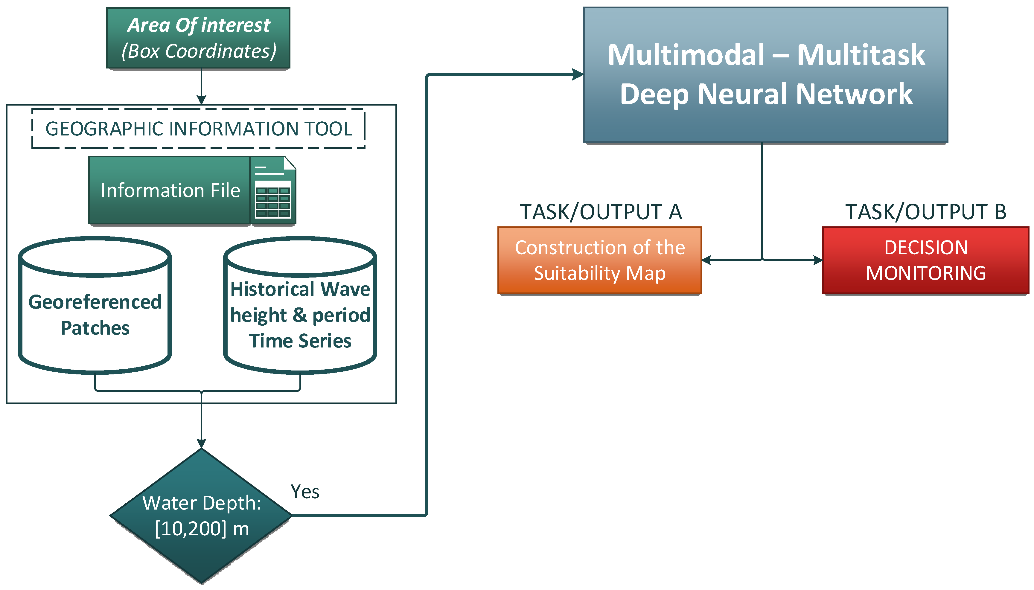
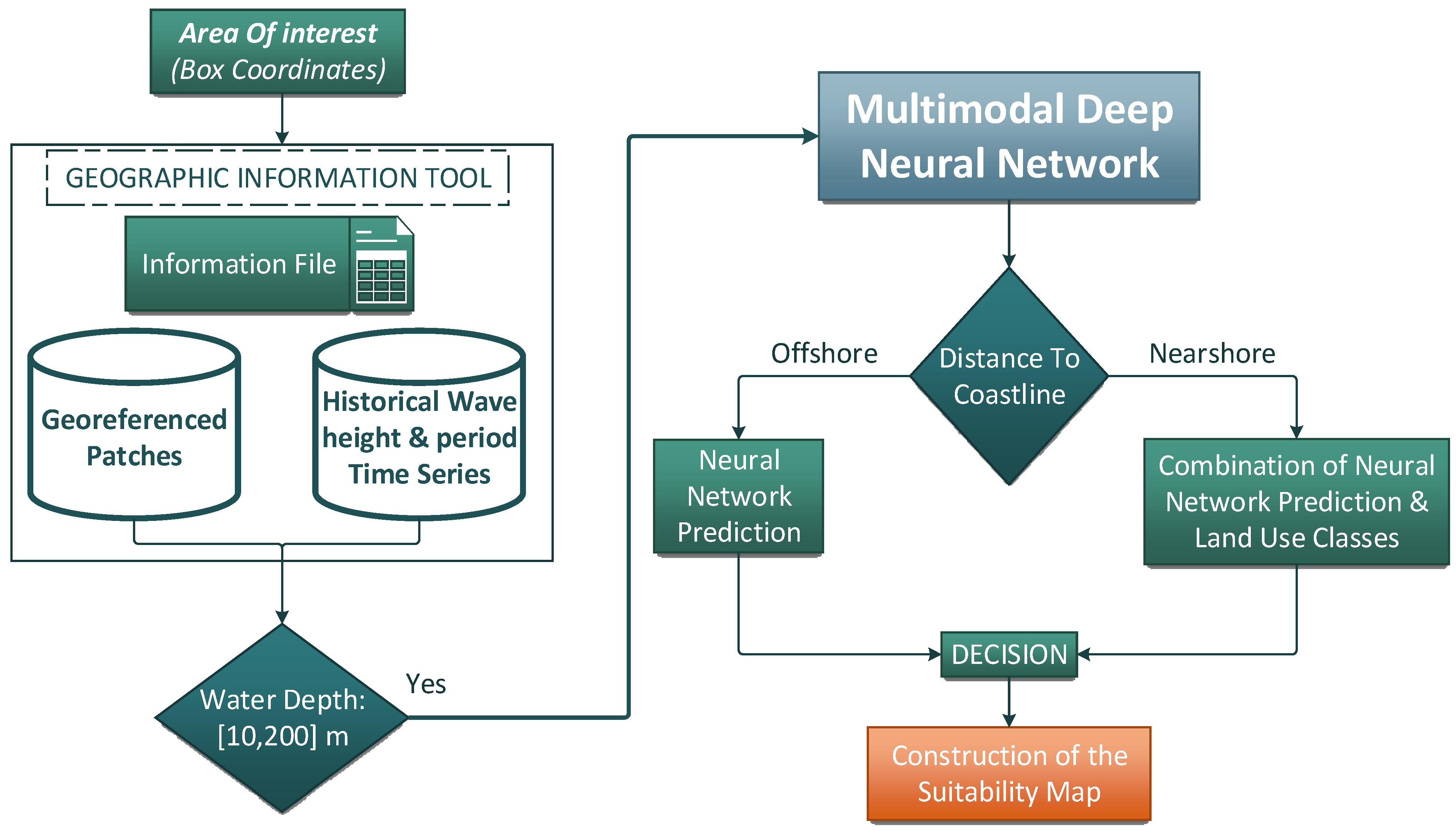
The extraction of specific geographic datasets is necessary in order to implement the proposed method. We developed a Geographic Information Tool, which is necessary to generate the training dataset and apply the methodology to the selected area of interest. In its general form, this tool uses bounding box coordinates of the area of interest as an input and defines the grid of the potential WEC installation points, as well as it incorporates the necessary data. The flowchart of this tool is shown in
Figure 1. Initially, we acquire the Sentinel-2 Tile [
28] for the corresponding geographical coordinate using the Open Access Hub API. Then, we define the grid of the potential points for WEC installation and we create the georeferenced patch of Sentinel-2 images for each of the patches using the geometric buffer operation. We receive bathymetric data from GEBCO [
29] and 12-year Wave Height and Period time series using 3 h time-step from ERA-5 dataset [
30] via the Climate Data Store (CDS) API. In addition, we interpolate bathymetric and time series data to our grid, via the CDS Toolbox. For nearshore potential regions we extract land use classes and their polygons from Corine Land Cover (CLC) dataset [
31].
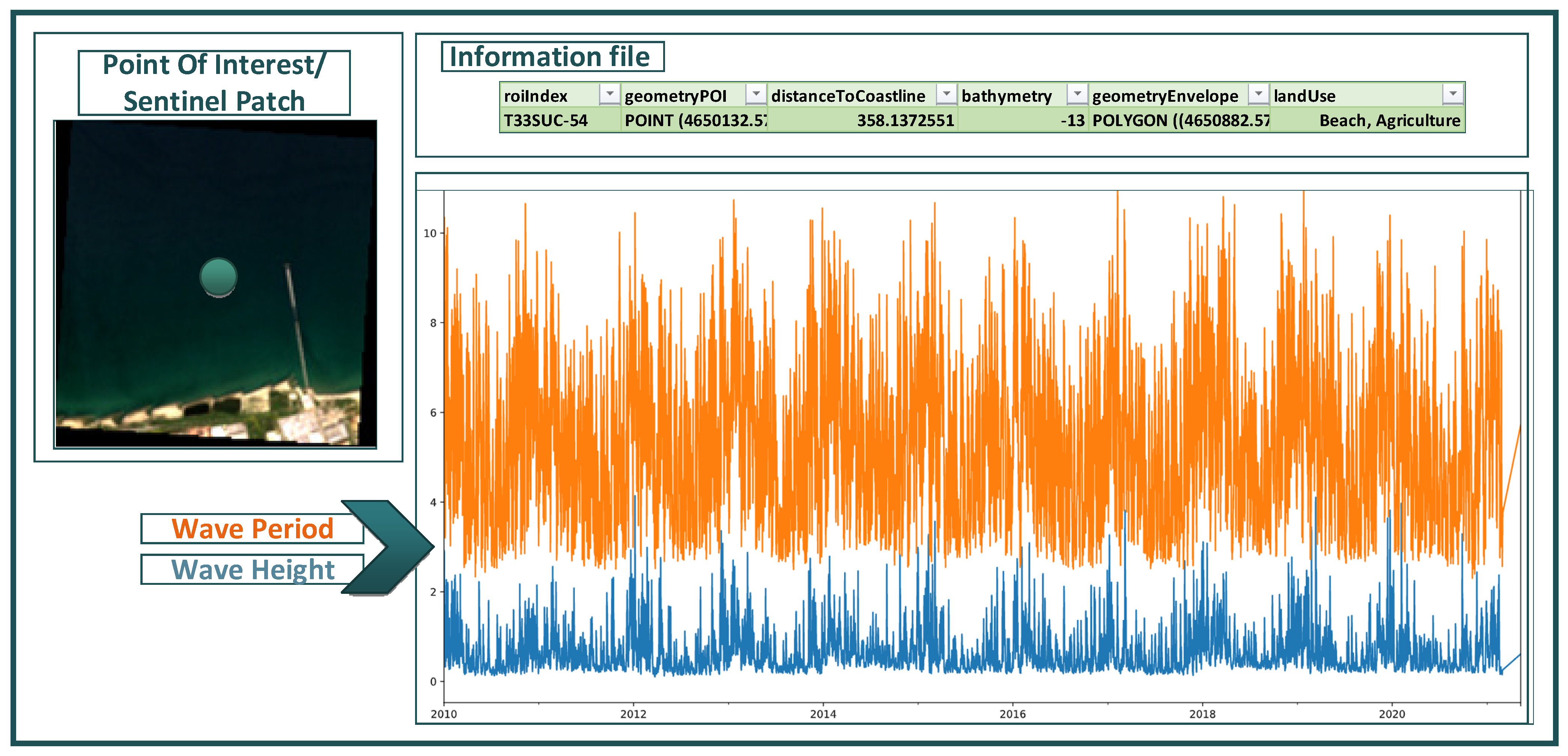
The output of our Geographic Information Tool is two databases connected via an information file. The first database contains the georeferenced image patches and the other one the historical wave height and period time series. In
Figure 2, an example of a potential WEC installation point is shown. In time series plot the
x-axis represents the 3-h time step for the past 12 years and
y-axis represents the values of Significant Wave Height (meters) and Peak Wave Period (seconds). Despite the fact that image patches and time series are stored to the corresponding database, the water depth and land use classes are stored in the information file.
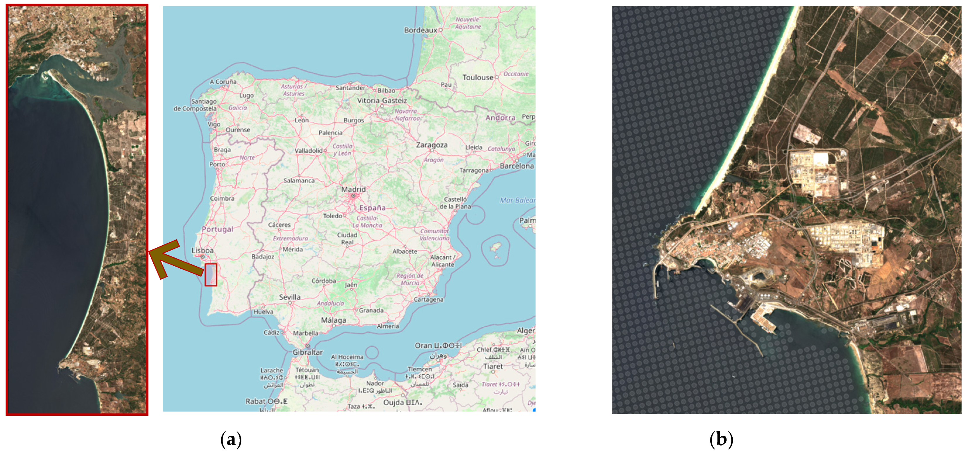
Generation of training dataset involves the labeling process of both satellite images and time series. More precisely, we must assign labels to image patches according to algae presence or absence. For this purpose, we use the algae presence observations from UNEP-WCMC dataset [
32,
33]. By extracting the potential WEC installation points with the aforementioned tool, the event dates from UNEP-WCMC records are used for the region of South Italy to acquire the corresponding Sentinel images. In this way, we used spatial intersection operation between seagrass and patches polygons to assign labels to potential WEC installation regions. On the other hand, time series labeling process is crucial for the assessment of the wave energy potential. In this paper, the novel method of Fairley et al. [
12] is used to assign labels about the wave energy. Particularly we implemented the W-based approach. Considering the Significant Wave Height (
Hs) and Peak Wave Period (
Tp) we calculate the Coefficient of Variation (
CV) of
,
. Precise,
CV is the ratio of standard deviation of a variable and its mean value. For each of the time series the following variables are calculated:
The aforementioned variables are used to cluster time series using K-Means (K = 6). According to Significant Wave Height cluster-mean we can sort clusters from 1 to 6 or low wave energy to high wave energy potential, respectively. Thus, we define the clusters 1 to 3 as unsuitable for WEC installation and the clusters from 4 to 6 as suitable. Finally, we can combine the above information in order to assign labels to potential WEC installation points as follows:
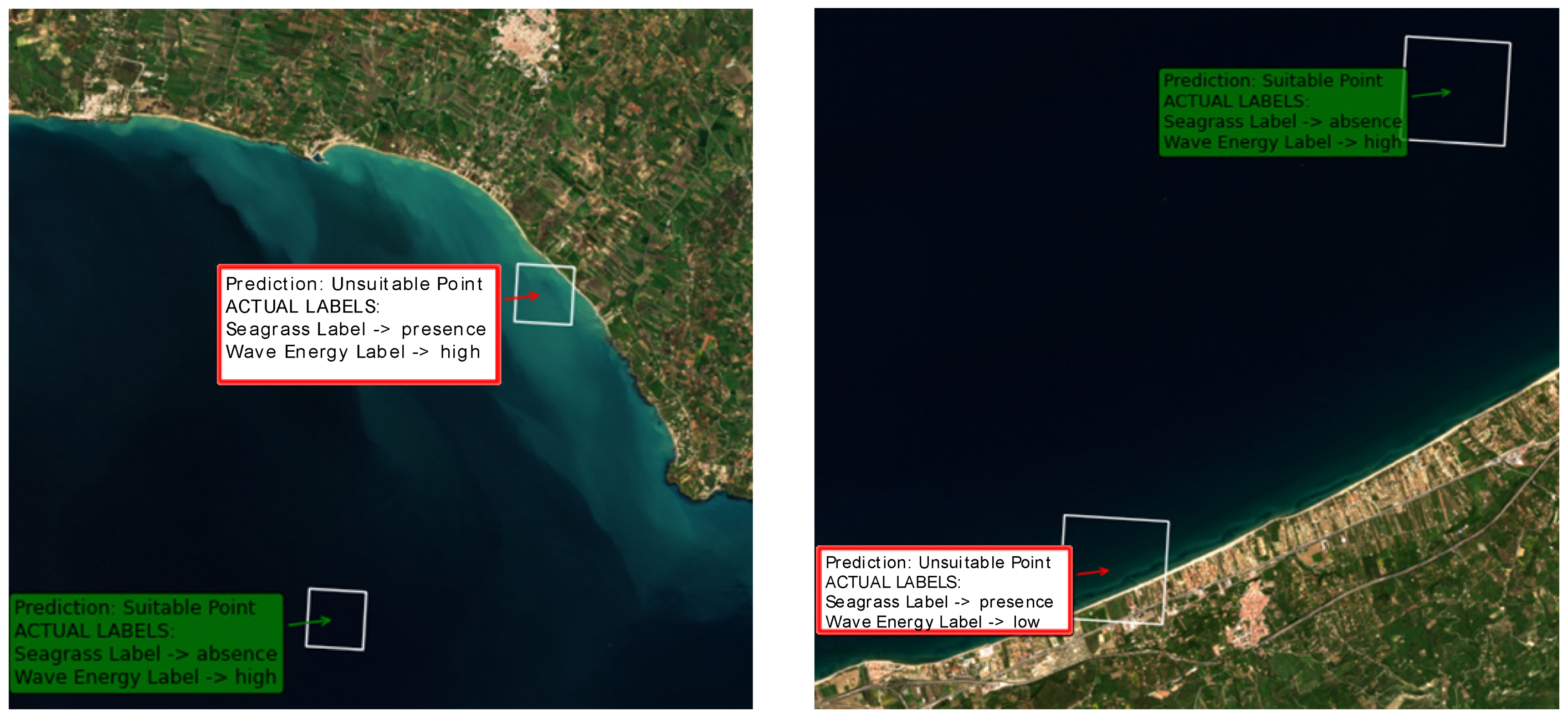
High Wave energy potential and Algae Absence means Suitable Area;
High Wave energy potential and Algae Presence means Unsuitable Area;
Low Wave energy potential and Algae Absence means Unsuitable Area;
Low Wave energy potential and Algae Presence means Unsuitable Area.
2.2. Deep Learning Algorithm
The proposed Deep Learning algorithm is the core of the system that we implemented to automate the process of WEC optimal positioning. As mentioned above, our system operates in two modes: In Mode I, we developed a Data Fusion based Neural Network. The image recognition branch only detects algae. The land use classes are received from a land use dataset. On the other hand, in Mode II, the image recognition branch classifies land use as well as the algae patterns. Thus, the potential regions classified as suitable or as not suitable for WEC installation is performed exclusively via DNN predictions. In this mode, we have implemented a Multitask Data Fusion based Neural Network. In both modes, we used heterogeneous data fusion techniques because the second branch of proposed architecture classifies wave height and period time series.
The Deep Learning model that we implemented is a Convolutional Neural Network (CNN), which is widely used for image recognition and is trained using the Backpropagation algorithm like the traditional ANN [
34,
35,
36,
37]. Besides this, CNN are efficient for time series classification [
38,
39]. Consequently, we developed a Convolutional architecture for each of two branches.
2.2.1. Data Fusion Based Neural Network
Consequently, we developed a Convolutional architecture for each of two branches. In order to create Multimodal DNN, its two branches are developed as individual Neural Networks. The reason leading to the specific implementation is to find the optimal architecture for each branch. One of the popular neural networks that work efficiently in the process of identifying marine algae in satellite imagery is the U-Net [
20]. This architecture is used for the Semantic Segmentation of an image. However, since we aim to classify images on the presence or absence of algae, an architecture inspired by the Encoder of U-Net is created, due to its efficiency in extracting features from images.
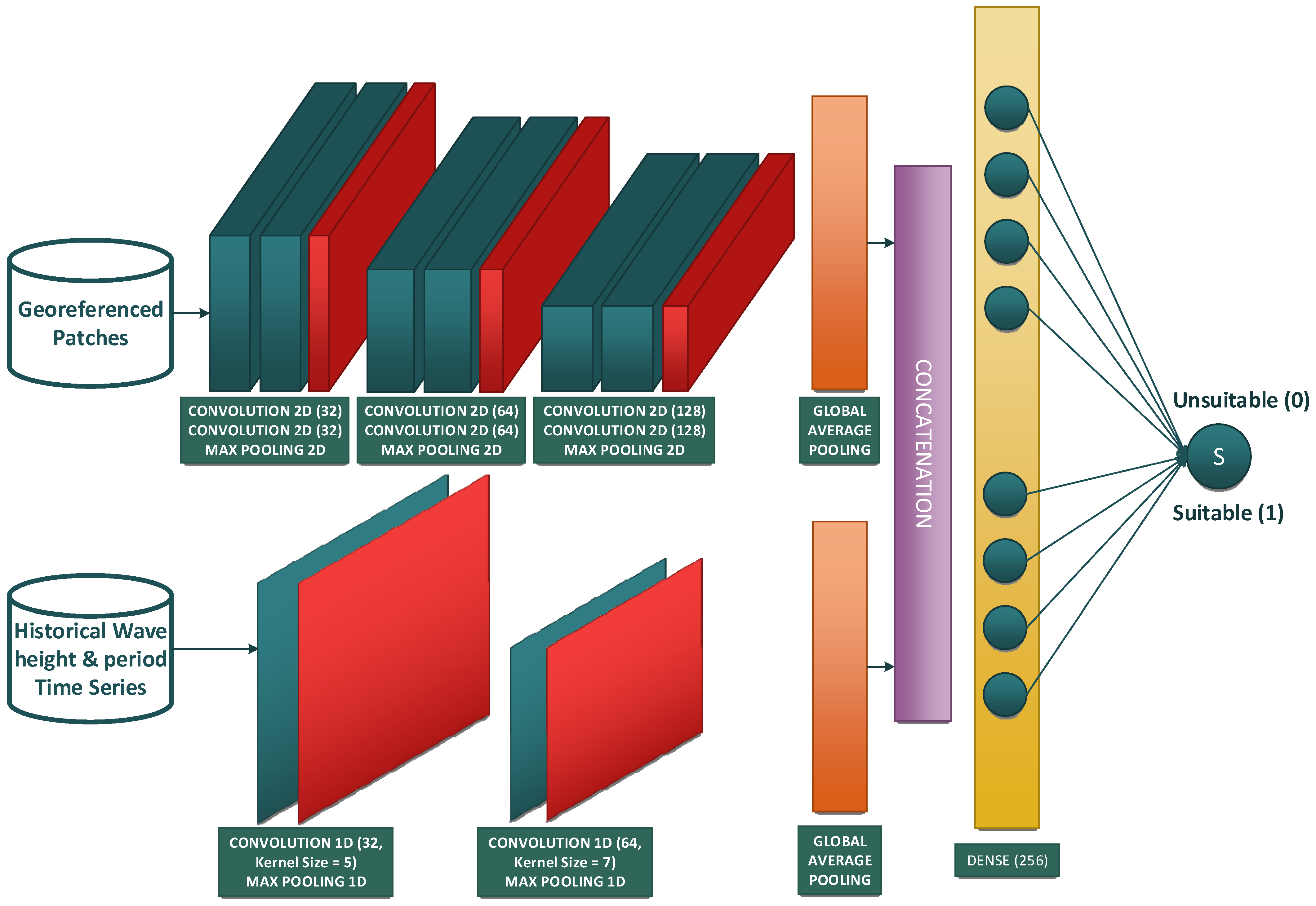
According to
Figure 3, the image recognition branch of the Neural Network has three convolutional blocks, in each of which two consecutive Convolutional Layers with the Relu activation function followed by Max Pooling are placed. The number of feature Maps defined per block is 32–64–128, respectively with a 3 × 3 filter. The Max Pooling process runs in 2 × 2 regions. At the final step, a Global Average Pooling (GAP) layer is used instead of the flatten operation. In this way, the average value is extracted from each feature map of the last convolutional node. GAP can replace the Fully Connected Layer, while helping to avoid overfitting because it reduces the number of training parameters. The time series branch of DNN consists of 1-D Convolutional and Pooling Layers. As it is shown in
Figure 3, this branch has one Convolution of 32 feature maps with a kernel size 5, followed by Max Pooling and then another Convolutional Layer with Filter size 7 from which 64 Feature Maps are extracted, followed again by Max Pooling of size 2. GAP Layer is used instead of Dense Layer too. The extracted features of the two branches are merged via the Concatenation Layer and this layer is fed to a Fully Connected Layer of 256 neurons which are activated via ReLU. Because the task is a Binary Classification problem, the Activation Function that is defined for the final neuron is the Sigmoid. The DNN is implemented on the Tensorflow and Keras Python libraries.
During the training process we need a heterogeneous-data fetching tool, which is developed using the Custom Data Generator of Keras and its input is the information file that connects the two databases (
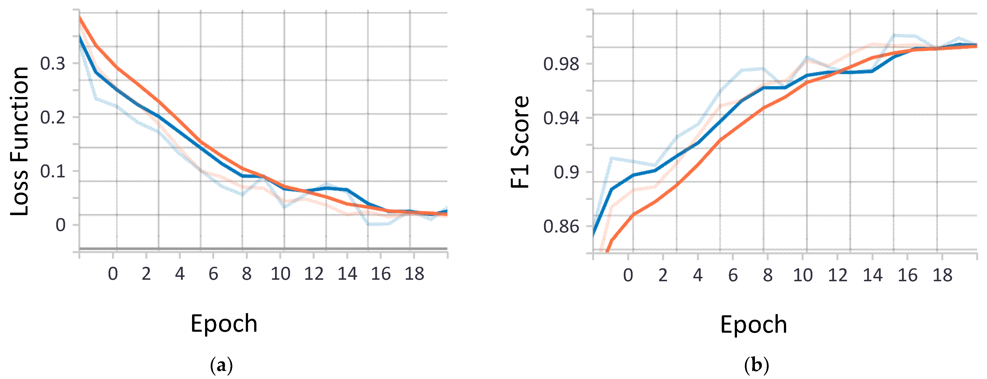
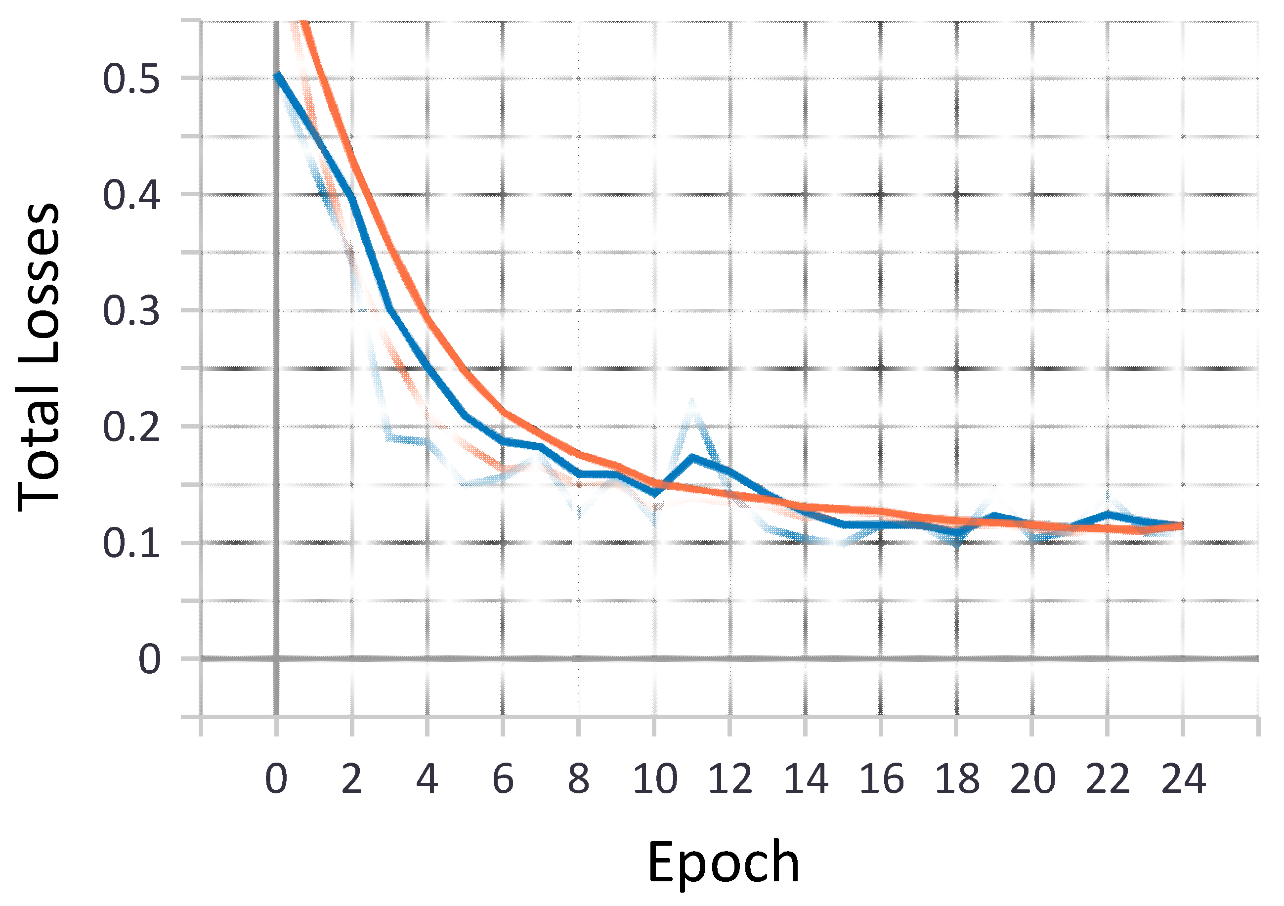
Section 2.1). Satellite images are normalized, dividing each pixel value with 255. The secondary input of Neural Network is a multivariate time series, in particular with two variables, for wave height and period, respectively. Thus, time series are modeled as a 2-D matrix, which consists of two columns, while the number of rows corresponds to the time-steps. Before starting the training process, we split the dataset using 60% for training, 20% for validation and 20% for testing. The validation dataset is fed to the Neural Network at the end of each epoch and when the value of the loss function during the prediction of the data does not improve further, Early Stopping occurs. The Dataset Test is used after the end of the training in order to verify the ability of Neural Network to be generalized. Finally, we use the Adam optimizer [
40], 16 batch size, Binary Cross Entropy (BCE) loss function and we estimate model performance according to Accuracy, Precession, Recall and F1 metrics. This Neural Network represents Mode I.
2.2.2. Multitask Data Fusion Based Neural Network
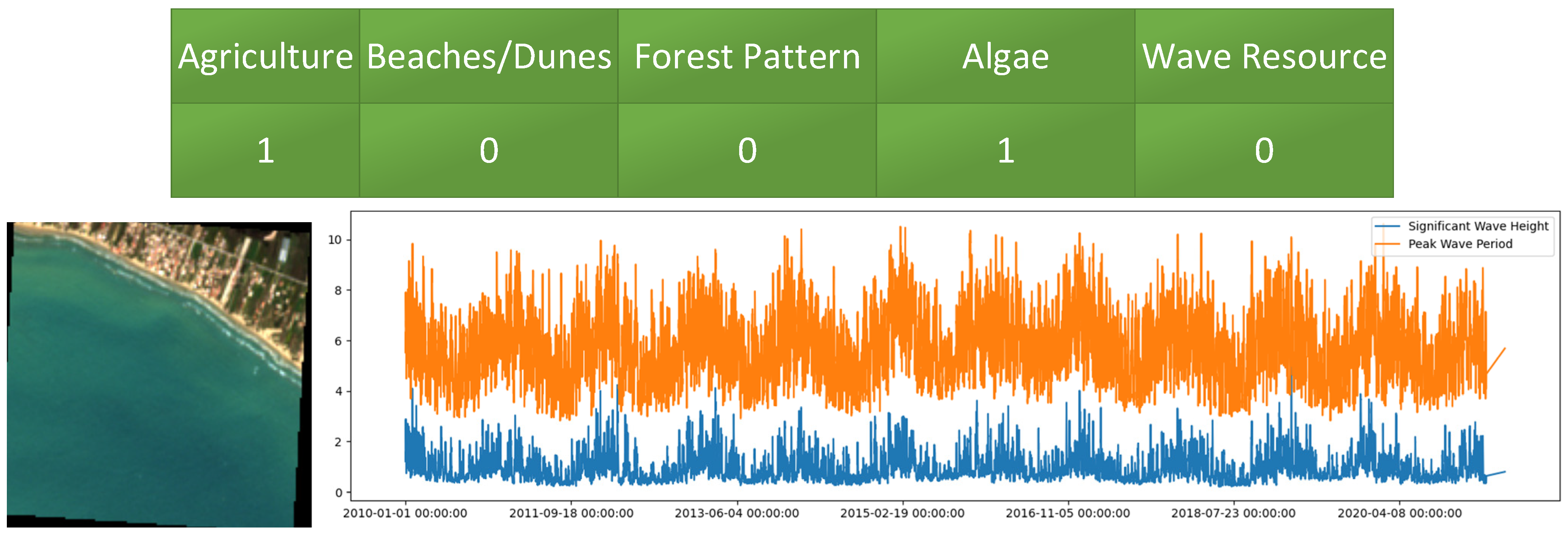
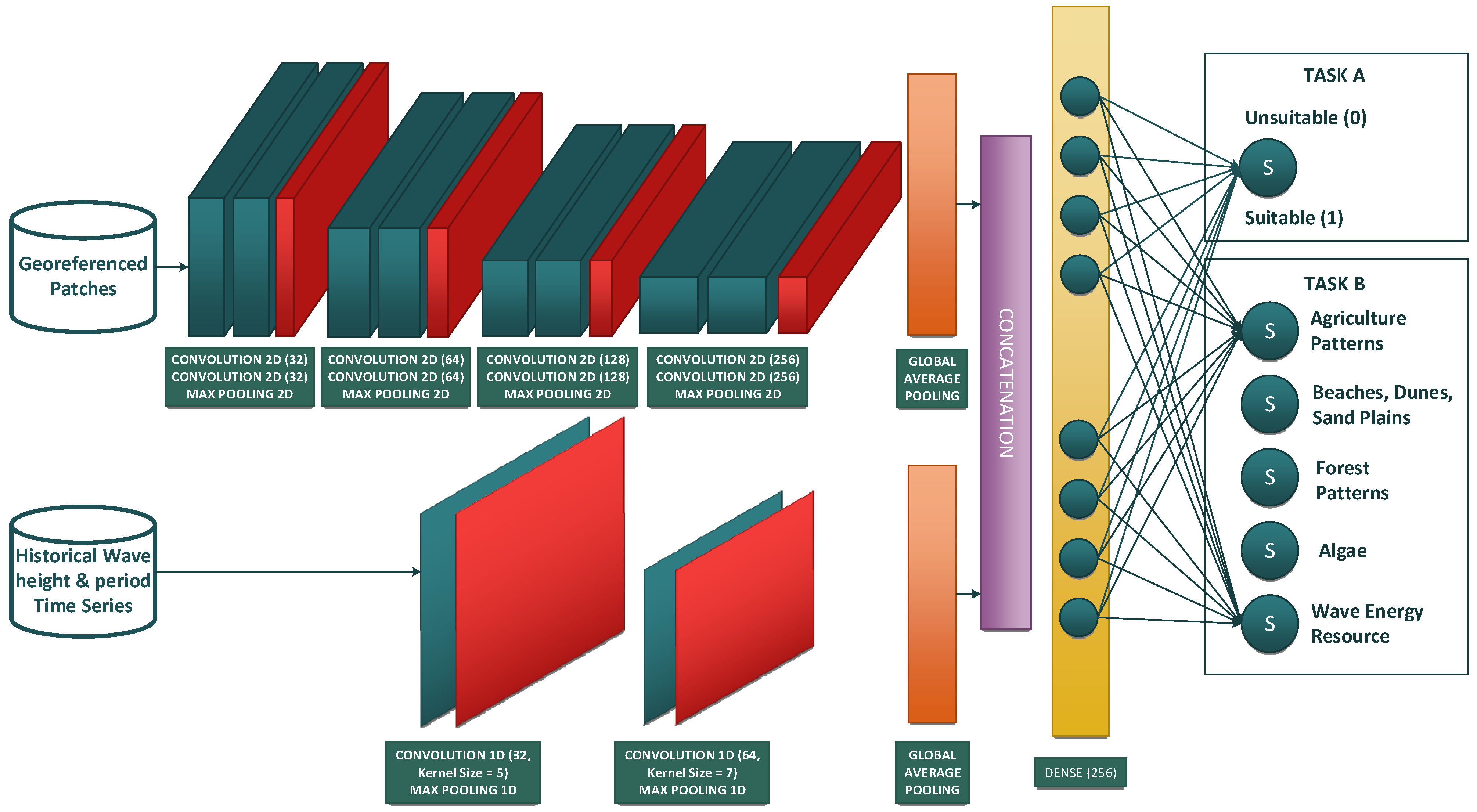
In this section, we present the Neural Network that constitutes the core of Mode II. Particularly, the process of land use classification via the image recognition branch is integrated. This implementation requires the adaptation of both the Neural Network architecture and the training dataset. At the first stage, we determined a One-Hot label for each of the potential WEC installation points. The first four cells of the corresponding table describe the geospatial constraints (Agriculture Activities, Beaches/Dunes, Forest Pattern and Algae) and the last cell is the suitability label of wave energy potential. We provide an example of One-Hot label in
Figure 4.
When the table has the value 1, then the corresponding class exists in the area. The last cell of the table concerns the wave energy assessment, and values 0 or 1 correspond to low or high wave energy, respectively. Based on the One-Hot table, each point is labelled as suitable or not for WEC installation. In this case, the encoding that implies a suitable point (Label equal to 1) is [0,0,0,0,1]. In any other case, the potential region is not suitable and the final label is equal to 0. In
Figure 4, an example of an unsuitable region for WEC installation is shown. In this case, we need to build a Neural Network for the solution of two tasks: Multi-label classification and Binary Classification.
When a neural network consists of two outputs, during backpropagation, the common weights are modified in order to optimize two loss functions in parallel. In other words, the model learns to recognize the suitability of a region based on which classes are recognized.
The architecture of Multimodal DNN is modified, initially, as the to the depth of the satellite image recognition branch. In particular, one more Convolution Block is added, and as a result, the number of Feature Maps defined per block are 32–64–128–256, respectively. The time series classification branch remains unchanged. After combining the extracted features from two branches through the Concatenation Layer, a Fully Connected Layer of 256 neurons is used. The first output is for the Binary Classification problem (suitable or not suitable WEC installation point), while the second is used to predict the above One-Hot table. We use BCE loss function on both outputs and we define the Accuracy metric and F1 score in order to estimate the performance of the Binary Classification and Multi-Label classification, respectively.
Figure 5 shows the Neural Network Mode II architecture.
2.3. Optimal Positioning of WECs Using Deep Learning—System Implementation
As mentioned before, the decision-making system for WEC positioning, is implemented through two modes, which differ in how the information related to the land use of coastal areas is obtained. In Mode I, the satellite imagery branch recognizes exclusively algae patterns which constitutes the dynamic component. Therefore, the prediction of the suitability of each potential point is based on both the presence or absence of algae and the energy availability of the region, which is classified through the time series branch. The output of the Multimodal DNN is combined with the CLC data in order to avoid additional geographic limitations. The variant in Mode II, is the recognition of land use/cover classes by the satellite image branch. In this case, the suitability of each potential WEC installation point is predicted via the DNN.
Common processes for both modes are the definition of potential installation points and the integration of the corresponding data (
Section 2.1). In addition, points that are not in the depth range between 10 and 200 m are excluded.
2.3.1. Mode I
The first implementation of the WEC installation positioning system is modeled according to the flowchart in
Figure 6. The Data Fusion based DNN of
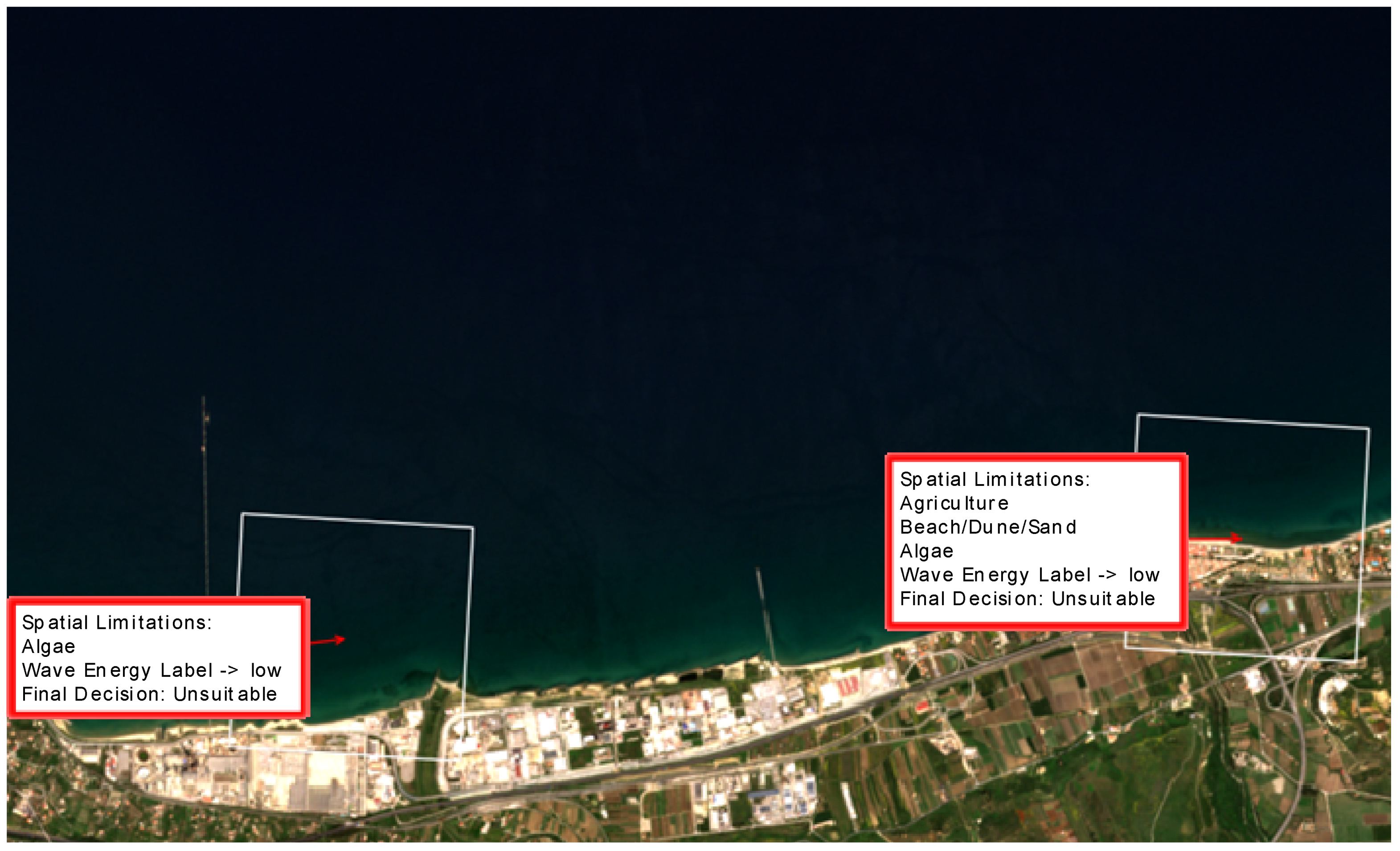
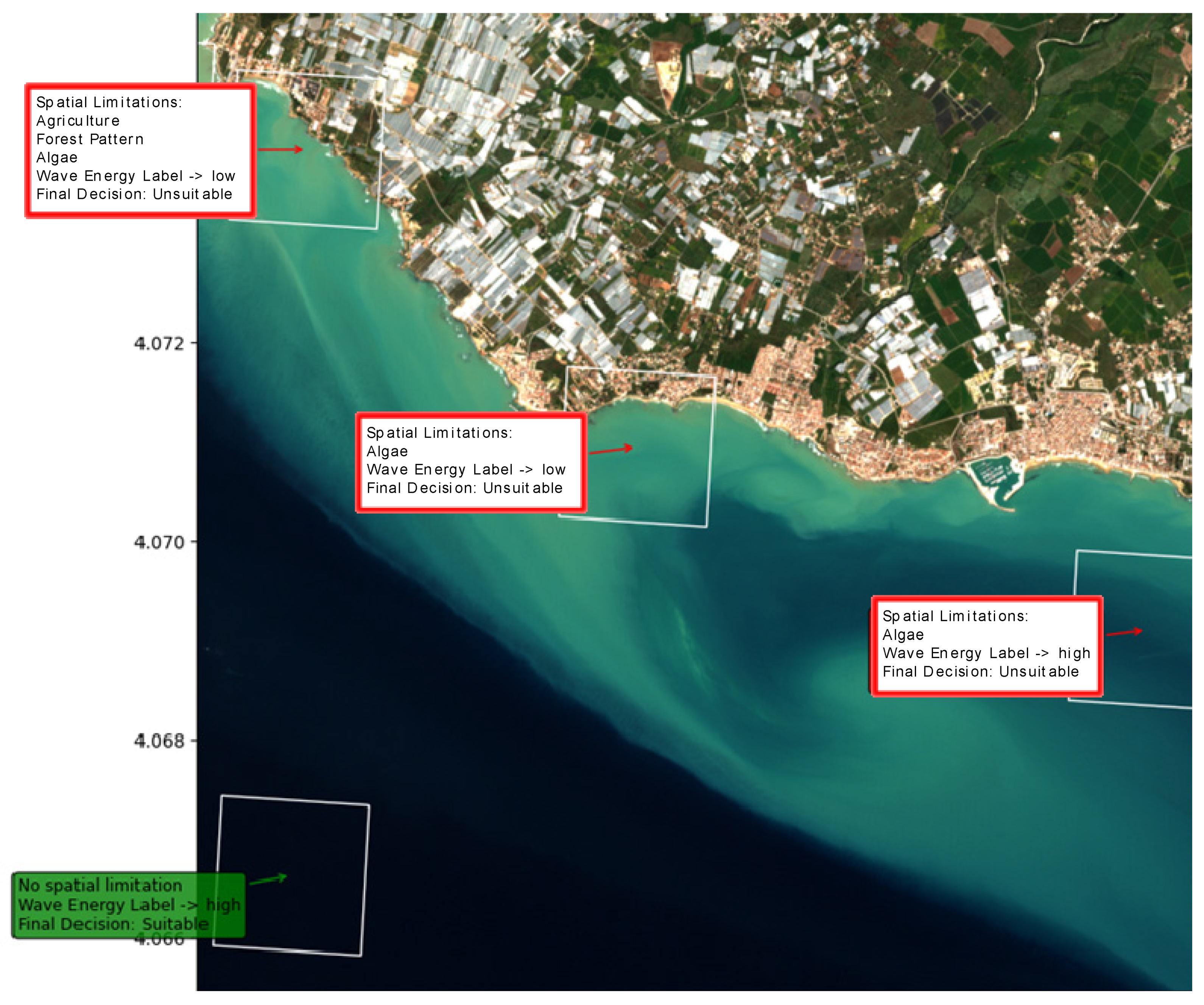
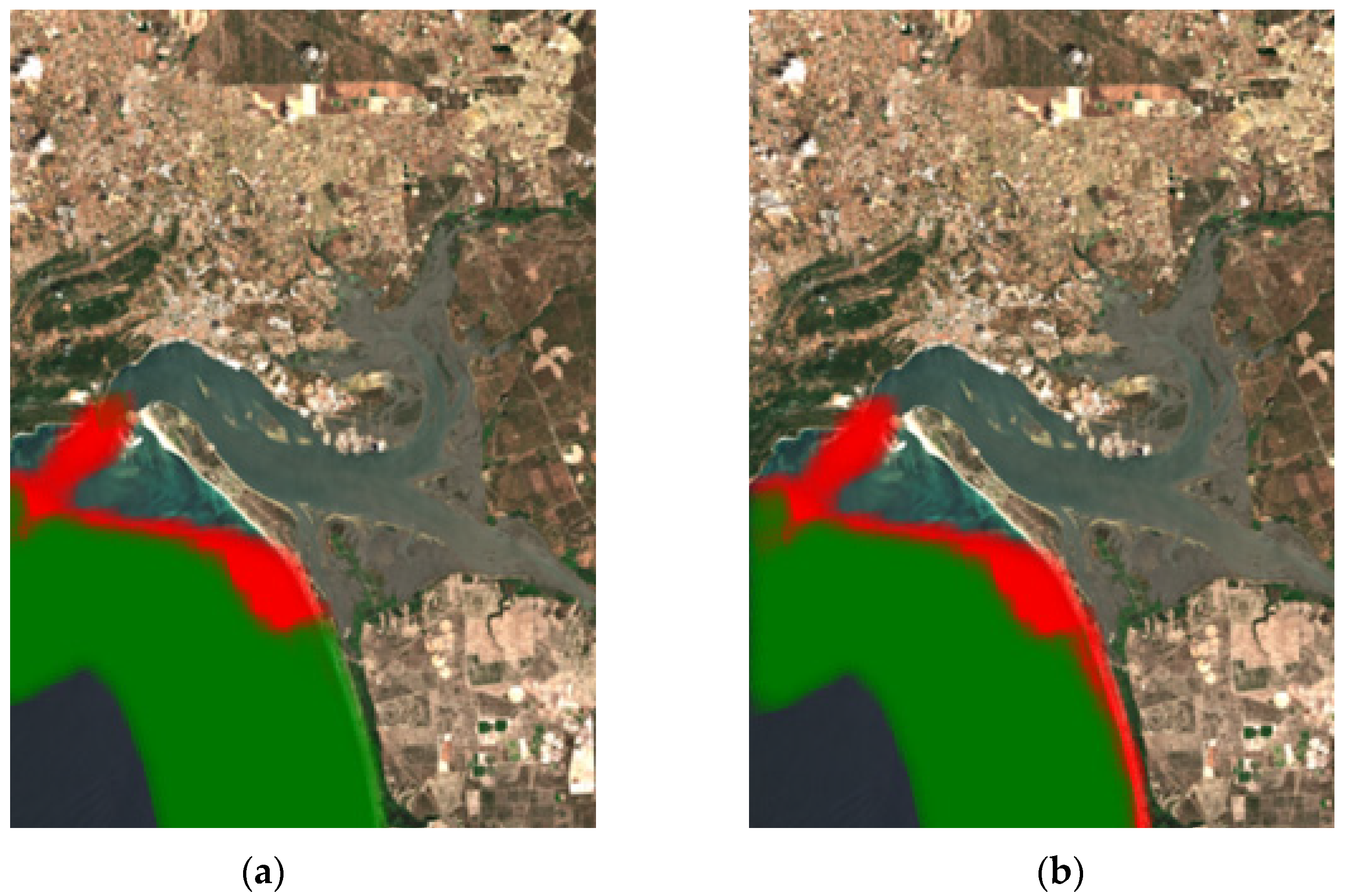
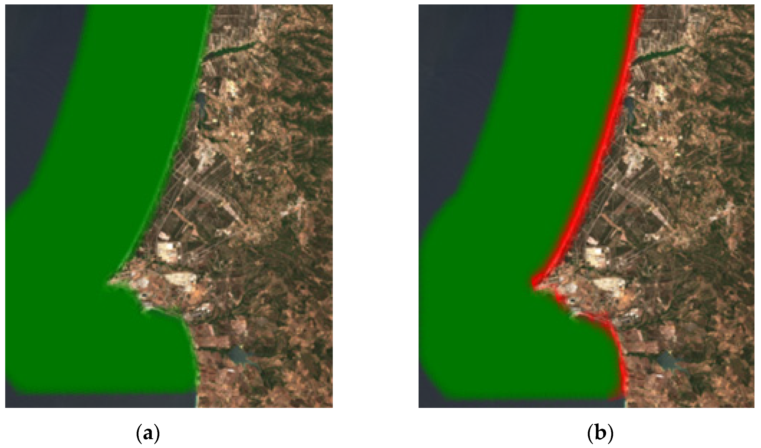
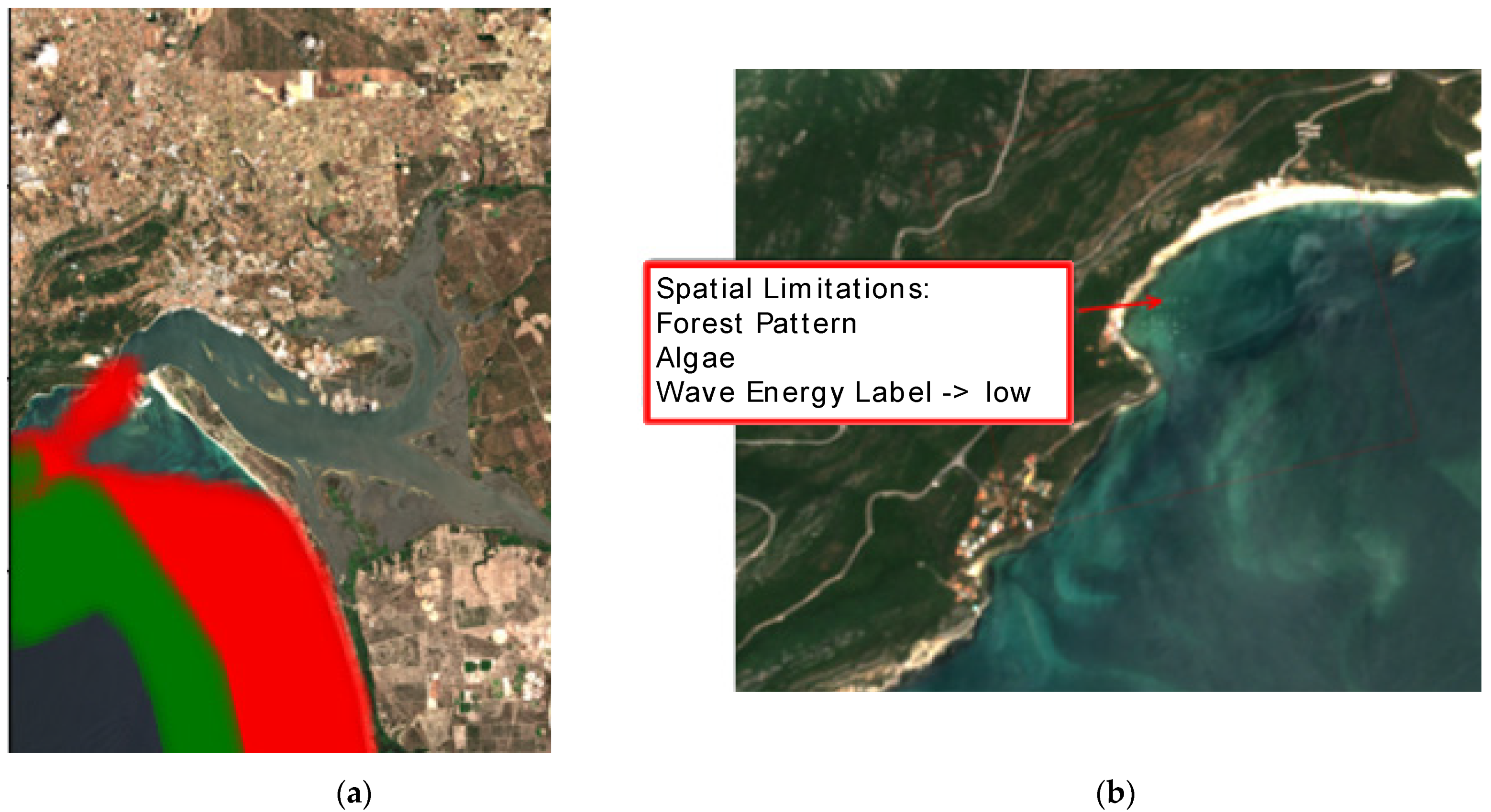
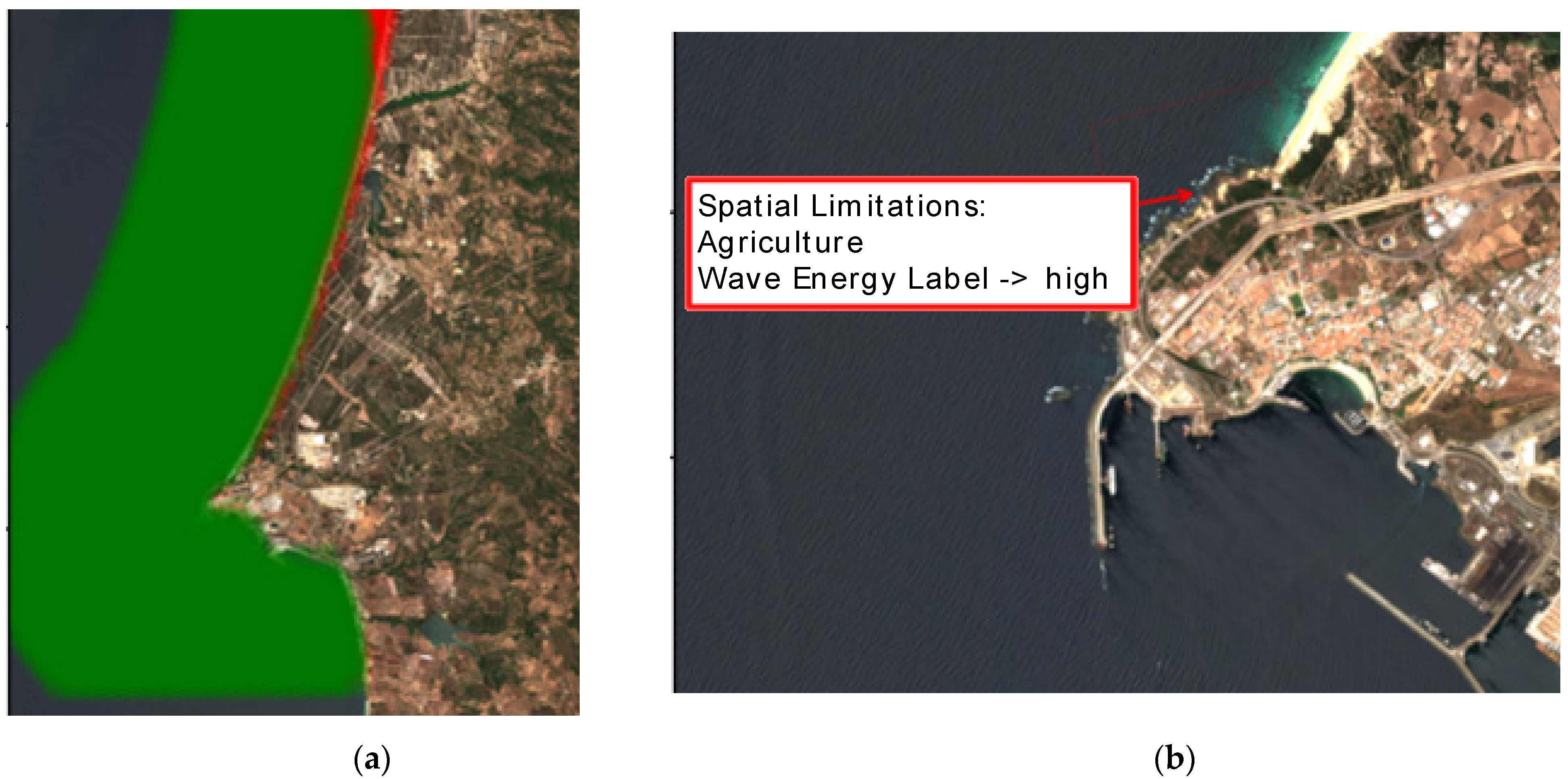
Section 2.2.1 takes the georeferenced Sentinel patch and time series as input and predicts the corresponding binary label. If the latter is zero, then the point is considered as not suitable for WEC installation. In contrast, prediction of suitable points implies both the absence of algae and high wave energy potential. In this case, the system further processes some information in order to make the final decision. In particular, if the potential region is offshore, then it is considered suitable for WEC installation, while if it is a nearshore point, it is required to avoid additional spatial restrictions related to the use/coverage of the closest coastal land. If in the latter beaches, swimming zones, dunes, woodland or agricultural facilities are located, then the point is automatically rejected. Finally, decisions of each of the potential WEC installation sites are combined, in order to construct the suitability map of the overall area of interest.
2.3.2. Mode II
The second mode of the WEC optimal positioning methodology contains the Multitask data fusion based Neural Network analyzed in
Section 2.2.2 as a core unit. In this way, the decision for each point is taken directly through the corresponding output of DNN, that is, the one that implements the Binary Classification problem. In addition, the output of the Multi-label Classification process is used to monitor how the final decision is formed, since as a result, the land use classes identified, including algae, as well as the energy suitability results are given. The flowchart of this process is in
Figure 7.
4. Conclusions and Discussion
This paper presents a new, Deep Learning-based methodology to automate the process of WEC optimal positioning. The presented models work with freely available satellite images, as well as Climate Reanalysis data. The methodology is applied through two different approaches. In Mode I, land use data are received from CLC dataset, while in the second method they are extracted from the satellite images in order to avoid additional geographic limitations. At the end of the training process, the model being developed is capable of identifying the spatial restrictions in satellite images, including algae patterns that are dynamically changing features. At the same time, the system estimates the wave energy potential by treating it as a dynamic phenomenon, which is characterized by non-predictable temporal variability. In addition, our model can identify the differences in temporal variability of multiple locations. In this way, it is confirmed that merging heterogeneous data works efficiently in solving complex problems. Thus, it turns out that CNNs are efficient in both image and time series recognition.
In this paper, we initiate a new method for the spatial positioning of WEC that is based in recognition of geospatial constraints which are dynamically changing patterns in marine areas. Thus, the main limitation of this study is the fact that additional dynamic classes can be added to satellite image recognition task. Under this rationale, the proposed model can be generalized to include several image-related dynamic phenomena. In marine areas there are characteristics that change in time, so their identification is difficult without Machine Learning or costly monitoring. In addition, the main technical challenge of this study is the fact that the examination of dynamic geospatial and technical restrictions should be combined in terms of Levelized Cost of Energy (LCOE) of wave energy and GIS methods [
45]. Regarding land use, the interconnection of the proposed system with an API such as Google Maps/Places or Open Street Map could be efficient because these platforms contain data that are frequently updated. Finally, in addition to assessing climatic conditions, a third branch can be added to the proposed Neural Network for time series forecasting.


