Hybrid Physics-Based Adaptive Kalman Filter State Estimation Framework

Abstract

State-of-the art physics-model based dynamic state estimation generally relies on the assumption that the system’s transition matrix is always correct, the one that relates the states in two different time instants, which might not hold always on real-life applications. Further, while making such assumptions, state-of-the-art dynamic state estimation models become unable to discriminate among different types of anomalies, as measurement gross errors and sudden load changes, and thus automatically leads the state estimator framework to inaccuracy. Towards the solution of this important challenge, in this work, a hybrid adaptive dynamic state estimator framework is presented. Based on the Kalman Filter formulation, measurement innovation analytical-based tests are presented and integrated into the state estimator framework. Gross measurement errors and sudden load changes are automatically detected, identified, and corrected, providing continuous updating of the state estimator. Towards such, the asymmetry index applied to the measurement innovation is introduced, as an anomaly discrimination method, which assesses the physics-model-based dynamic state estimation process in different piece-wise stationary levels. Comparative tests with the state-of-the-art are presented, considering the IEEE 14, IEEE 30, and IEEE 118 test systems. Easy-to-implement-model, without hard-to-design parameters, build-on the classical Kalman Filter solution, highlights potential aspects towards real-life applications.

1. Introduction

Electric power systems are critical infrastructures that rely on continuous and detailed monitoring of their assets, encompassed by power system state estimation (PSSE). Since its conception in the early 1970s, PSSE has been focused on processing the steady-state condition of the transmissions systems, under a static analysis framework [1]. With the penetration of renewable energy and new control equipment, the static perspective does not provide the modern energy management systems’ requirements. Thus, it becomes imperative to capture systems’ dynamics for advanced automated applications, in such a way to provide fast control actions, increase the reliability of the system, diagnosis of cyber-attacks, and optimize resources across the power grid [2,3,4].

Dynamic state estimation in power systems can be understood as to estimate the grid states, as voltages magnitude and phases, considering the time relation between them. There are many presented physics-model-based dynamic state estimation (DSE) solutions, being the Kalman Filter formulation and it is likewise a family of formulations most used [3,5,6]. The first formulations of DSE in power systems were proposed shortly after the consolidation of static state estimation in transmission system operation centers [7,8,9,10,11,12].

Such works established the theoretical foundations to capture the dynamic characteristic of the power system. They encompass a first-order state-space model to represent the temporal relationships among the state variables and the Kalman Filter technique application. However, the computational burden of the algorithm, and the lack of fast updating measurements in the Supervisory Control and Data Acquisition (SCADA) system hindered real-life applications [3,5,12]. Only in the late 2000s, dynamic state estimators regained significant interest, with the advent of faster computer architectures, by the allocation of new instrumentation and communication technologies with faster updating and sampling rates, and as well as the acute power system operational requirements, carried by a more volatile environment with renewables [5]. In the effort of surpassing many of the practical and theoretical challenges, different versions of the Kalman Filter were proposed, such as the Linear Kalman Filter [13], the Extended Kalman Filter [14], the Unscented Kalman Filter [15], the Cubature Kalman Filter [16], the Correntropy Kalman Filter [17] and the Ensemble Kalman Filter [18]. Nonetheless, all such approaches consider a single stationary scenario or that only known load changes occur on the system. This translates to the assumption that the system’s transition matrix is always correct, which might not hold in real-life applications. In a complementary perspective, robustness against measurement gross errors for dynamic state estimators gained a significant research effort. The work in [19] shows that incorporating the state-space model can benefit classical bad-data processing based on the weighted residual analysis. Also, recent works seek to improve the estimator robustness by changing its objective function, such as by the M-estimators [20], the generalized maximum likelihood estimation [21], the weighted least absolute value [22], the H-infinite [23] and hybrid approaches [24]. Altogether, robustness is often obtained at the cost of improving the estimator variance, computational burden, or model complexity. Conversely, such approaches fail to discriminate measurement gross errors from changes in the stationary load level, often treating them in the same theoretical perspective, or by modifying the residual-based tests. Amidst such a promising challenge, this work explores a family of Kalman Filters formulation for the DSE problem. The state space is modeled under a piece-wise stationary state space, and the change in the stationary load level must be detected and discriminated from measurement errors. Towards such a goal, a statistical asymmetry index, applied to the system innovation, is introduced. This metric is used in analytical-based tests towards continuous discrimination of anomalies type. In this work, it is further shown that considering the condition of changing the stationery load level, the asymmetry index will have a non-zero small value. In this case, the innovation will not have Normal distribution. Otherwise, in the measurement gross error condition, the innovation will present a large asymmetry index, due to the modeling structural discontinuity. Therefore, the presented analytical-based tests enable discrimination among different types of anomalies and automatically adapt the dynamic state estimator to maintain accuracy. The specific contributions of this work towards the state-of-the-art are：

• The development of a hybrid state estimator framework, based on the Kalman Filter formulation, able to diagnosis measurement gross errors and sudden load changes automatically;
• The exploration of the asymmetry index as an anomaly discrimination method, assessing the DSE process in different piecewise stationary levels, which can be used in any family of Kalman Filters-like dynamic state estimators framework.

The remaining of the manuscript is structured as follows: Section 2 presents the theoretical background for DSE and the Kalman Filter (KF). Section 3 introduces the dynamic estimator and the innovation analysis for anomaly discrimination. Section 4 presents test results, followed by the conclusions, which are presented in Section 5.

2. Dynamic State Estimation

DSE in power systems can be understood to estimate the grid states, as voltages magnitude and phases, considering the time relation between them. DSE in power systems can be modeled as

$$\begin{array}{cc}\hfill {\underline{x}}_{k+1}& =F_k{\underline{x}}_k+G_k{\underline{\mathrm{w}}}_k+{\Gamma }_k{\underline{u}}_k\hfill \\ & {\underline{z}}_k=H_k{\underline{x}}_k+{\underline{v}}_k,\hfill \end{array}$$

(1)

With ${\underline{x}}_k$ the state vector at time k, ${\underline{\mathrm{w}}}_k$ a known input and ${\underline{u}}_k$ the state noise. Equivalently, ${\underline{z}}_k$ the observation vector and ${\underline{v}}_k$ the observation, or measurement, noise. $F_k$ is the state transition matrix, $G_k$ is the matrix relating the states to the input ${\underline{\mathrm{w}}}_k$ and $H_k$ is the matrix relating measurements to states at time k, all of them with the appropriate dimensions. Figure 1 illustrates a block diagram for the signal model with external known input that corresponds to the DSE problem.

Within the power systems realm, dynamic state estimation has been conceptualized under different perspectives, mainly related to the definition of state variables. The fundamental difference comprises the inclusion, or not, of internal variables from generators and loads (also referred to as dynamic state variables), besides the complex nodal voltages of the power network (also referred to as algebraic state variables) [3,5]. The first focuses on fast transient events that may cause instabilities, while the second on slower rates of change that affect the loading condition of the power networks. Nonetheless, both represent a system subject to a stochastic phenomenon and uncertainty. The difference lies in the time scale of events and observed response of the system. In this work, dynamic state estimation refers to the second definition, also referred to as tracking or forecasting-aided state estimation [4], focused on the power flow behavior over time, that is, the temporal relations among different operational conditions of the interconnected power grid. Hence the state variables comprise the complex nodal voltages in all nodes of the power systems $x=\{(V_i,{\theta }_i)|i\in \{1,2,\dots ,n_{bus}\left\}\right\}$. The measurements comprise electrical quantities monitored in real-time by the SCADA systems. A detailed discussion about the employed models and physical aspects of the power system is presented in the Appendix A.

2.1. Statement of the Discrete Kalman Filtering Problem

Considering the linear, finite-dimensional, discrete system described by the previous equations, with ${\underline{v}}_k$ and ${\underline{\mathrm{w}}}_k$ being independent, Gaussian white noise processes with

$$E\left[{\underline{v}}_k{\underline{v}}_j^T\right]=R_{k}andE\left[{\underline{\mathrm{w}}}_k{\underline{\mathrm{w}}}_j^T\right]=Q_k,$$

(2)

where $R_k$ is the measurement noise covariance matrix and $Q_k$ is the state covariance matrix. Suppose ${\underline{x}}_0$, the initial value of the system state variables, being a Gaussian random variable. Assuming they have mean ${\overline{\underline{x}}}_0$ and covariance matrix ${\sum }_{0|-1}$, the KF solution consists of estimating ${\underline{x}}_{k|k-1}$ and ${\underline{x}}_{k|k}$ and their associated error covariance matrices ${\sum }_{k|k-1}$ and ${\sum }_{k|k}$. Here ${\underline{x}}_{k|k-1}$ means estimating the state vector at time step k with data until time step ($k-1$). If the assumption of a Gaussian distribution for ${\underline{x}}_0$, ${\underline{\upsilon }}_k$, and ${\underline{\mathrm{w}}}_k$ is dropped, but they remain described by their first and second-order statistical moments of their probability distribution functions, all the conclusions about unbiasedness and algorithm formulation are precisely the same. However, optimality, in the sense of the minimum variance estimator and minimum squared error, will not be the case. This is one of the major motivations to overcome gross errors in the measurement vector, that largely distort such assumption of Gaussian noise and negatively affects the estimation.

2.2. Solution of the Kalman Filtering problem

The KF model can be solved in two steps: the prediction and the estimation step.

(1) SKF Prediction Step:

The Kalman Filter prediction step is given by

$${\widehat{\underline{x}}}_{k+1|k}=F_k{\widehat{\underline{x}}}_{k|k-1}+K_k[{\underline{z}}_k-H_k{\widehat{\underline{x}}}_{k|k-1}]+{\Gamma }_k{\underline{u}}_k,$$

(3)

With ${\widehat{\underline{x}}}_{0|-1}={\overline{\underline{x}}}_0$. The Kalman gain is given by:

$$K_k=F_k{\sum }_{k|k-1}{H}_k^T{\left[Hk{\sum }_{k|k-1}{H}_k^T+R_k\right]}^{-1},$$

(4)

the inverse is guaranteed with $R_k$ being a positive definite matrix, while the conditional error covariance matrix ${\sum }_{k|k-1}$ is computed recursively by the Riccati equation:

$${\sum }_{k+1|k}=F_k\left[{\sum }_{k|k-1}{H}_k^T{(H_k{\sum }_{k|k-1}{H}_k^T+R_k)}^{-1}{H}_k{\sum }_{k|k-1}\right]F_k^T+G_k{Q}_k{G}_k^T,$$

(5)

where, ${\sum }_{k+1|k}$ is the updated error covariance matrix.

(2) KF Estimation Step:

The KF estimating solution is given by

$${\widehat{\underline{x}}}_{k|k}={\widehat{\underline{x}}}_{k|k-1}+{\sum }_{k|k-1}{H}_k^T{(H_k{\sum }_{k|k-1}{H}_k^T+R_k)}^{-1}({\underline{z}}_k-H_k{\widehat{\underline{x}}}_{k|k-1}),$$

(6)

assuming that the inverse exists, the error covariance matrix is given by

$${\sum }_{k|k}={\sum }_{k|k-1}-{\sum }_{k|k-1}{H}_k^T{(H_k{\sum }_{k|k-1}{H}_k^T+R_k)}^{-1}{H}_k{\sum }_{k|k-1}.$$

(7)

2.3. Bad Data Analysis

Considering DSE, besides measurement errors, one can have other anomalies as large load changes. In this case, the state transition matrix may not reflect the hull transition of states. This highlights the difficulty in modeling the system for DSE purposes. The state uncertainty can be quantified by white Gaussian noise with covariance $Q_k$. This technique may incur some difficulties: if one assumes a high covariance so that the sudden load change is inside the modeling, the estimate may be significantly poor for the case of small load fluctuations. Otherwise, if the noise covariance is considered small, to represent well the small load fluctuations, the model will not simulate large load fluctuations, but, in this case, it could be used to identify the anomaly for large load variations [10].

To tackle the previous challenge, in this work, as the state-of-the-art, the state transition matrix is modeled through an identity matrix, with a small covariance matrix. This will represent a stationary system behavior. As a tradeoff, possible changes in the stationarity load level will be detected. However, measurement gross errors could be misidentified as a stationarity level change. Sudden large load changes, as well as measurement gross errors, will be named here as an “anomaly”. That said, they are anomalies of different characteristics and should be, in this way, automatically detected and identified. One should note that in the bad data condition, there exist equations “inconsistencies” or “a structural discontinuity” of the equations describing the DSE behavior [10,25]. Otherwise, considering the large load changes, there is no structural discontinuity in system equations [10,17,25]. In this work, the distinction between these anomalies is done through the analysis of the statistical distribution of the innovation process.

Due to the structural discontinuity in the equations, the innovation for the measurement gross error condition will present a large asymmetry characteristic. Otherwise, considering stationarity load level changes, the symmetry related to the innovation average value will keep its value, but dislocated from zero. In this case, the innovation will not have a Normal distribution [10]. These characteristics are illustrated in Figure 2.

3. Dynamic State Estimation Formulation for Gross Error Analysis

The power system state can be defined by an n-dimensional $\underline{x}$ vector consisting of the voltages magnitudes and their phase angles, except one of them, taken as reference. The system state can be modeled as

$${\underline{x}}_{k+1}={\underline{x}}_k+{\underline{\mathrm{w}}}_k.$$

(8)

With ${\underline{\mathrm{w}}}_k$ being a white Gaussian, noise vector with

$$E\left[{\underline{\mathrm{w}}}_k{\underline{\mathrm{w}}}_j\right]=Q_{kj}andQ={\alpha }^{2}diag\left(q_i^2\right)={\alpha }^2\Gamma .$$

(9)

The previous $q_i$ is the maximum ratio of the state i obtained from historical data of bus i. To represent power flows, the measurement model in power systems dynamic state estimation consists of the following set of nonlinear equations $\left(h\left(x_k\right)\right)$ given by

$${\underline{z}}_k=h\left({\underline{x}}_k\right)+{\underline{\upsilon }}_k.$$

(10)

and

$$E\left[{\underline{\upsilon }}_k{\underline{\upsilon }}_j^T\right]=\left[{\delta }_{kj}{R}_{kj}\right],E\left[{\underline{\upsilon }}_k\right]=\underline{0}.$$

(11)

The estimate $\widehat{\underline{x}}$ of $\underline{x}$ is obtained using the Kalman filter theory:

$${\sum }_{k+1|k}={\sum }_{k|k}+Q_k$$

(12)

$$K_k={\sum }_{k|k}{H}_k^T{[H_k{\sum }_{k|k-1}{H}_k^T+R_k]}^{-1}$$

(13)

$${\widehat{\underline{x}}}_{k|k}={\widehat{\underline{x}}}_{k|k-1}+K_k[z_k-h\left({\widehat{\underline{x}}}_{k|k-1}\right)]$$

(14)

$${\sum }_{k|k}=[I-G_k{H}_k]{\sum }_{k|k-1}$$

(15)

With $H_k$ the Jacobian matrix of $\underline{h}$ computed at $\underline{x}=\widehat{\underline{x}}$.

The hull differentiation between the anomalies, gross error, and sudden load change, will be based on the deformation of the innovation distribution function [10]. In the following, the Innovation process is introduced. While using an analytical model, the implicit hypothesis is that system behavior is considered stationary by parts.

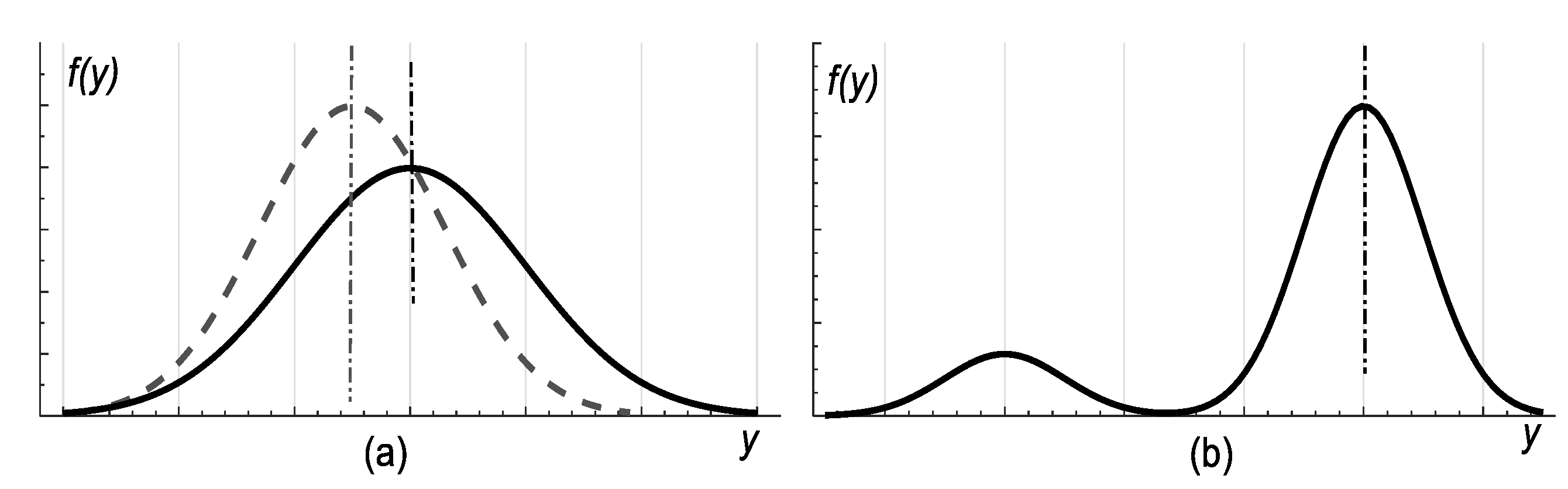
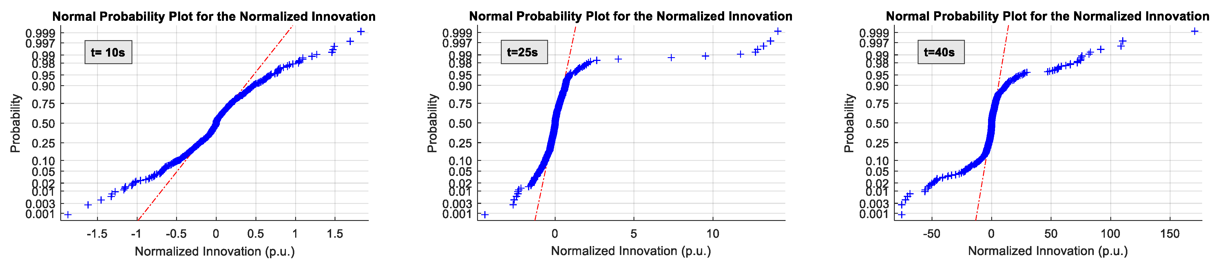
3.1. The Innovation in the Dynamic State Estimation Process

The system innovation is modeled by

$${\underline{\upsilon }}_k={\underline{z}}_k-\underline{h}\left({\widehat{\underline{x}}}_{k|k-1}\right)$$

(16)

As one knows, ${\upsilon }_k$ is a white Gaussian process, so that:

$$E\left[{\underline{\upsilon }}_k\right]=0,E\left[{\underline{\upsilon }}_k{\underline{\upsilon }}_j^T\right]=H_k{\sum }_{k|k-1}{H}_k^T+R_k.$$

(17)

Normalizing the innovation process, one obtains:

$${\lambda }_{k,i}={\lambda }_{k,i}/{\rho }_{k,i}$$

(18)

$${\rho }_{k,i}^2=H_k{\sum }_{k|k-1}{H}_k^T+r_{k,i}^2$$

(19)

where ${\underline{\upsilon }}_{k,i}$ is the $ith$ component of ${\underline{\upsilon }}_k$ and $H_{k,i}$ is the $ith$ line of $H_k$. In this way, one can define the random variable ${\Lambda }_k$ (the set of all individual innovations ${\underline{\upsilon }}_{k,i}$) whose sample is the normalized innovation process, presents a normal distribution with average zero and unitary covariance. Considering the bad data condition, this would not be in fact an innovation, since the innovation probability function would change. Otherwise, considering the stationary level change, that would be the case, since the probability function would be dislocated from zero, but still a normal distribution [10].

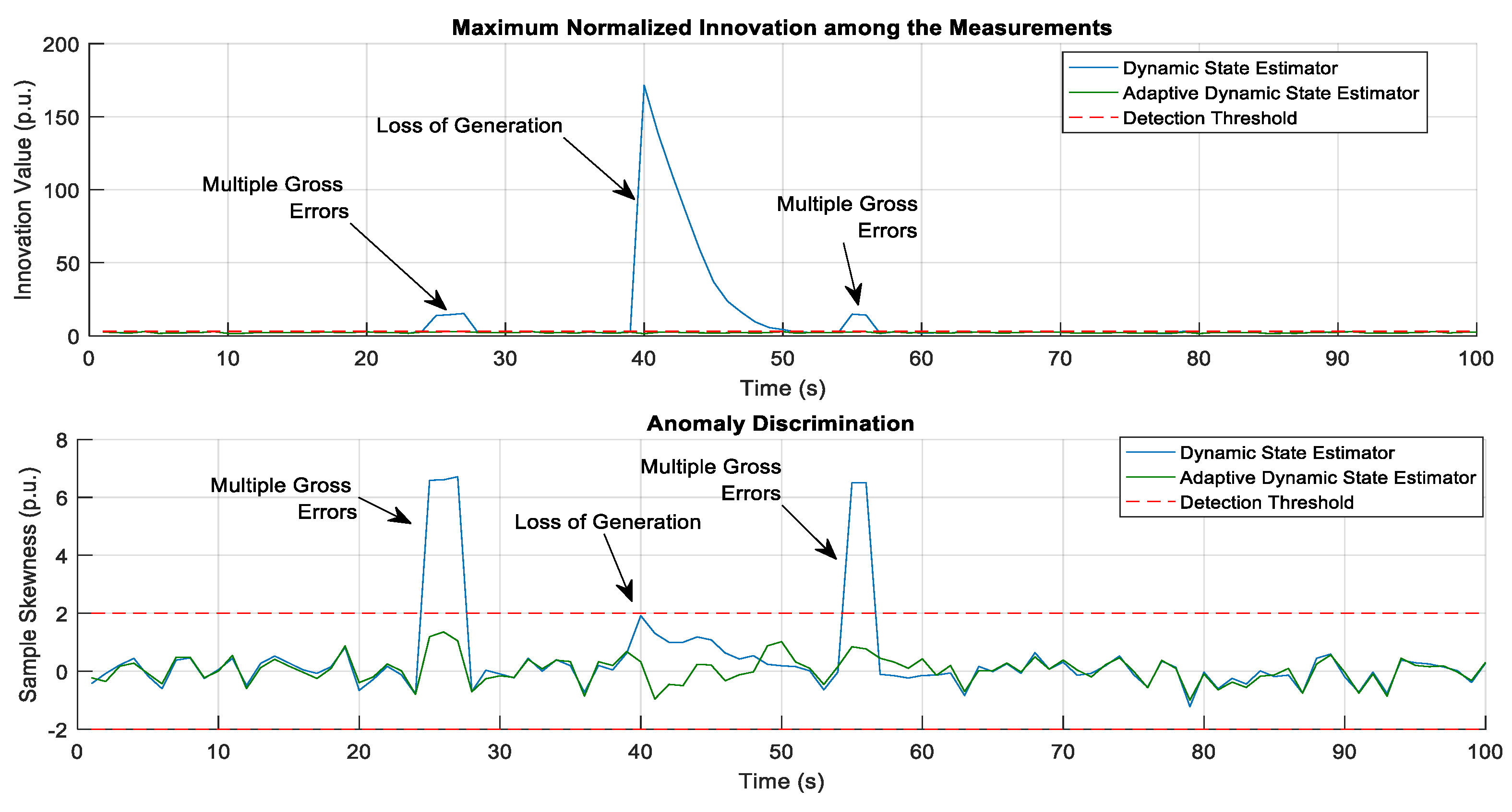
3.2. Anomaly Detection

In this work, two types of anomalies are considered, that is, the sudden change of system states and measurement gross errors. Considering the measurement value ${\underline{z}}_k$, in a measurement gross error condition, the predicted state value will present significant errors in the innovation Equation (16) [10,25].

When this anomaly occurs, the innovation distribution ($\Lambda$) in the normalized form is considerably different from the $\Lambda$ distribution for the case of stationarity level change, as illustrated in Figure 2, where f($\lambda$) is the probability distribution function for $\lambda$ [10]. If those measurements are deleted or corrected, considering the measurement gross error condition, the distribution for $\Lambda$ is equivalent to the stationary case situation. Otherwise, for the abrupt stationary level changes case, a significant number of elements of the innovation process are affected, and the Gaussian behavior will stay valid, but with an average magnitude, not zero, that is, the symmetry related to the non-zero average value will stay valid, which does not occur for the measurement gross error condition. The detection of sudden load changes is mainly related to the sensitivity of the state variables to the active and reactive power injections of each bus of the system. Thus, the detection of anomalies in a specific node may be more difficult if the system is less sensitive to it, for instance, buses with the smallest loads. On the contrary, it will be more sensitive to variations in buses with more loads or generation. The main factor in such detection feature is the tuning of the state covariance matrix $Q_k$ of the Kalman Filter. The elements of the covariance matrix should reflect the impact on the state variables caused by the expected load and generation variations. Considering the previous, in this work anomalies will be detected by the test:

$$|{\lambda }_{k,i}|<\alpha ,i=1,2,\dots \dots n$$

(20)

With $\alpha$ a chosen threshold value (in this work assumed equal 3.0). This value is chosen considering the desired significance level and degrees of freedom. If at least one element of the innovation process is out of the pre-specified region, an anomaly condition is characterized.

3.3. Anomaly Discrimination and Adaption

The anomaly discrimination is in this work done by estimating the deformation of the innovation distribution. This deformation is estimated by the asymmetry index of the innovation distribution related to the average [11]:

$${\gamma }_k=M_{3,k}/{\sigma }_k^3,$$

(21)

With $M_{3,k}$ the third moment of the distribution, at time k, and ${\sigma }_k^3$ the standard deviation of that distribution. The third moment is given by

$$M_{3,k}=E\left[{\Lambda }_k^3\right]-3{\mu }_{k}E\left[{\Lambda }_k^2\right]+2{\mu }_k^3$$

(22)

With

$${\sigma }_k^3=E\left[{\Lambda }_k^2\right]-{\mu }_k^2,{\mu }_k=E\left[{\Lambda }_k\right]$$

(23)

When the innovation deformation tends to zero, the distribution is symmetric and the constant ${\gamma }_k$ tends to zero, as in the normal distribution. That said, for the measurement bad data condition, the distribution deformation is large, and then ${\gamma }_k$ becomes large as well, as symmetry is lost. Otherwise, for an abrupt change in the stationary level, the symmetry is not lost and ${\gamma }_k$ will have a low value. Thus, considering the ${\gamma }_k$ calculation for the normalized innovation, the anomaly will be discriminated by

• ${\gamma }_k>\left|{\gamma }_{max}\right|\to$ Measurement Gross error situation
• ${\gamma }_k<\left|{\gamma }_{max}\right|\to$ Suddenly state variable change

where, ${\gamma }_{max}$ is a threshold obtained by experience and at the same time by simulations (in this work assumed equal 2.0). This value is well-chosen considering a level of confidence and degrees of freedom. Toward surpassing the effects of anomalies in the state estimation, an adaptive analytical model is presented. The end goal is to restore the accuracy of the estimation process. The adaptive analytical model consists of two tests:

• If a gross error is detected (if $|{\gamma }_{k,i}|\ge \alpha$ and ${\gamma }_k\ge |{\gamma }_{max}\left|\right)$, the measurement with the largest normalized innovation is not considered, and the estimation process is repeated without this measurement;
• If a gross error is detected (if $|{\gamma }_{k,i}|\ge \alpha$ and ${\gamma }_k<|{\gamma }_{max}\left|\right)$, the estimation considers only the current snapshot of measurements, thus not considering the time relations between states, and the estimation process is repeated using a static estimator:

4. Presentation of Performed Tests and Analysis of Results

This section describes the performed tests and analyses for the presented anomaly detection model. The algorithm behavior for anomalies identification, through the asymmetry index of the distribution curve of the innovation, is presented. The simulation methodology includes random noise in the results of a reference scenario to emulate the measurement set. A load flow calculation obtains the reference scenario, and the measured values are given by (24) [26]. The power system’s temporal aspect is simulated by a sequence of power flow scenarios, each instant with its corresponding loading/generation scenario. Each sample represents a different discretized instant k and the respective measured values. Thus, the simulation consists of a sequence of quasi-stationary conditions. Gross errors are included in the measurements by including larger error values in a specific set of measurements. Anomalies in the power system are simulated as sudden changes in the reference load flow scenario, changing the load/generation values and considering slow dynamic effects between successive instants. Measurements are considered with a sampling rate of one sample per second, a typical period of practical operation and supervisory systems.

$${\underline{z}}_{k,i}=z_{k,i}^{ref}+{\mu }_i\frac{p{r}_i\left|z_{k,i}^{ref}\right|}{3}$$

(24)

where $z_{k,i}^{ref}$ is the reference value for the $ith$ measurement at time k obtained by the load flow solution, $p{r}_i$ is the metering device precision (assumed as 2% for active and reactive power and 1% for voltage magnitude), and ${\mu }_i$ is a random value obtained from the standard Gaussian distribution. A similar equation also provides the diagonal elements of the measurement noise covariance matrix $R_{ii}=p{r}_i\left|{\underline{z}}_{i,k}\right|/3$. The process noise covariance matrix was calculated in a similar manner, by associating a percentage of admissible variation for each state variable in two successive instants ($\alpha$), the maximum state ratio in (9), according to a percentage of the previous state value $\left(x_{i,k-1}\right)$, that is

$$Q_{ii}={\alpha }^2{q}_i={\left(\alpha x_{i,k-1}\right)}^2$$

(25)

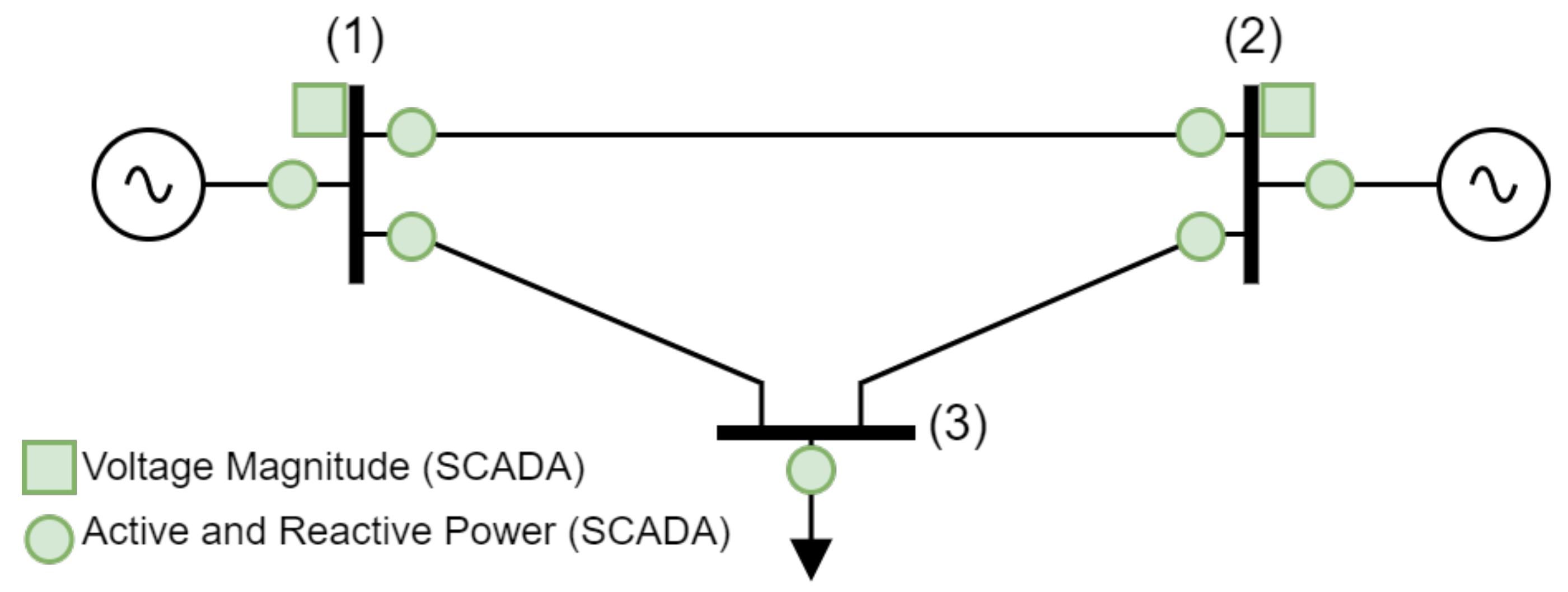
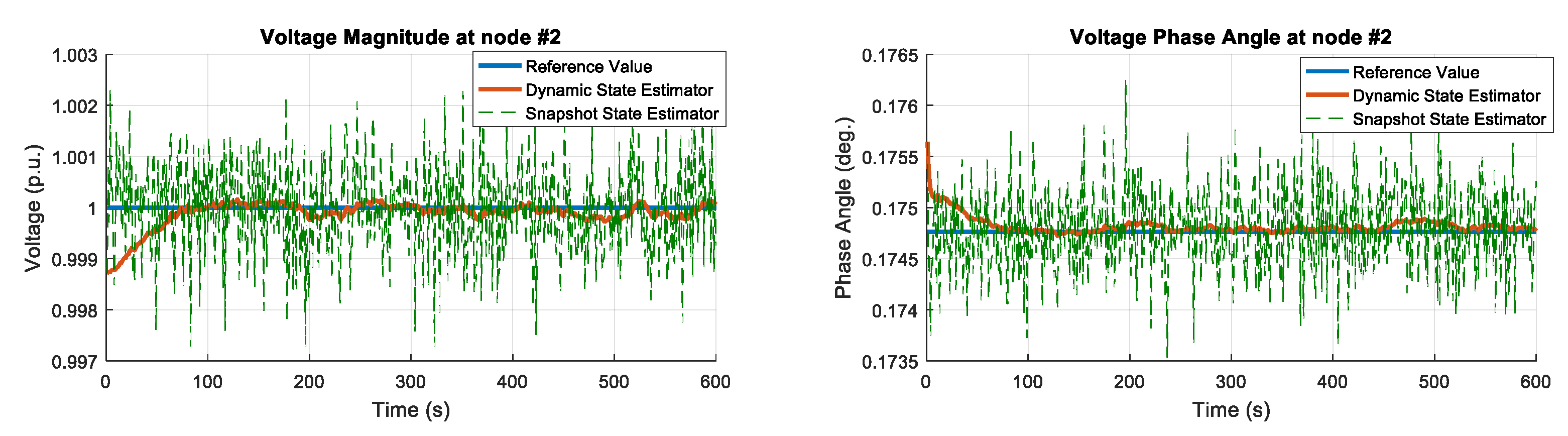
4.1. Conceptual Example and Asymptotic Performance of DSE

This section presents the initial simulation with a 3-bus test system, illustrated on Figure 3, as a conceptual example. The network data and reference loading scenario are provided in Appendix B. This simulation intends to show two main aspects of DSE in power systems, and the importance of supporting the algebraic state variables with the state-space model.

The state vector and measurement vector are defined by the following electrical quantities of the network, with the voltage phase angle at bus #1 as reference $({\theta }_1=0^0)$:

$$x={[V_1,V_2,V_3,{\theta }_2,{\theta }_3]}^T$$

(26)

$$z={[P_1,P_2,P_3,Q_1,Q_2,Q_3,P_{1-2},P_{1-3},P_{2-1},P_{2-3},Q_{1-2},Q_{1-3},Q_{2-1},Q_{2-3},V_1,V_2]}^T$$

(27)

The measurement model $h\left(x\right)$ in (9) is built according to the respective monitored electrical quantities. The temporal relations are included in the model as described in (8), that is, with an Identity matrix as a transition matrix. The measurement covariance matrix is a (16 × 16) diagonal matrix with elements obtained according to the respective measurement precision. While the state process covariance matrix is a (5 × 5) diagonal matrix with each element calculated according to (25), using a state rate equal to 0.01%.

In this test, the simulation consists of a stationary load condition under 10 min, with samples acquired at each second, to illustrate the asymptotical behavior of the Kalman Filter in comparison with traditional static state estimation, that is neglecting temporal relations among state variables. Figure 4 illustrates the state variables at bus #2 during the simulation. It illustrates the major conceptual enhancement of dynamic state estimation algorithms, an asymptotical improvement of the estimated values over time. Such advantage is valid under stationary conditions, as shown in the next simulations.

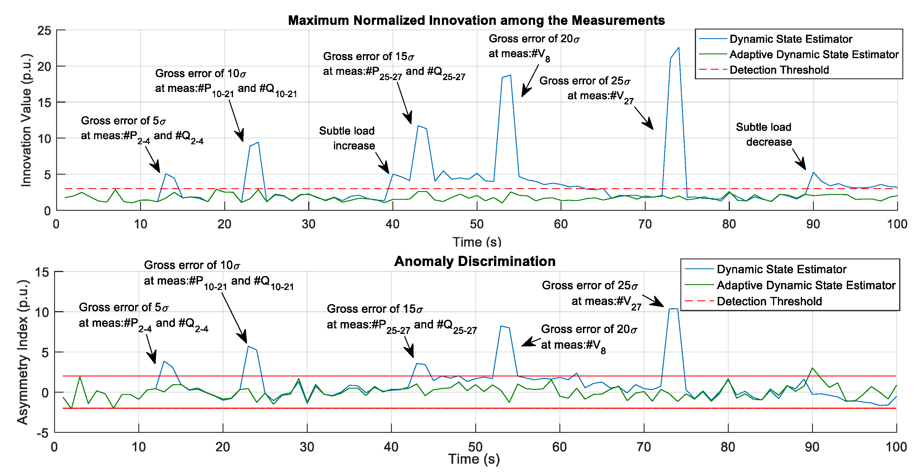
4.2. Performance of the Adaptive Dynamic State Estimator Algorithm

This section presents the application in the IEEE 14 test system [27] with the measurement set illustrated in Figure 5. The simulation consists of an initial stationary load condition under the first 20 s. A load increase at a constant rate of 0.2% per second follows from t = 20 s to t = 60 s, that is, a load ramp for all nodes, followed by more than 10 s of stationary condition. Then a sudden load increase of 5.0% occurs from t = 70 s to t = 90 s at four specific nodes (nodes #3, #4, #13, and #14). The state ratio in this test case was assumed as 0.03% of the previous state variable value.

Figure 6 presents the estimated state variables for node #14 in comparison to the reference load flow during this simulation. Figure 7 presents the estimation error boxplot between the estimated state variables and the reference values from the load flow calculation.

As one can see from the figures, when anomalies occur in the system, the estimation process deteriorates, especially for the phase angle. This is though expected, as, during such events, the hypothesis that the state transition matrix is equal to an identity matrix becomes false, that is, there is a change in the stationarity level of the system. Moreover, the proposed adaptation strategy successively identifies and adapts the estimator to each change on the stationarity level and in the presence of gross errors.

The adaptation strategy is triggered during the load ramp, at time steps #26s, #35s, #44s, and #54s. This is because the load ramp is a persistent anomaly, at that time during 40 s, which continuously changes the stationarity level of the system behavior during that interval. That said, the sudden load change (load increase and load decrease) are sudden changes that occur in a single instant, at time step #70s and #90s. In this case, the anomaly needs to be suppressed only once, in the instant of the load change, and the dynamic state estimator will return to the correct and new stationary level in a normal way. Figure 8 illustrates maximum absolute innovation value from all measurements and the calculated asymmetry index, in each instant.

One can see that, after the inclusion of measurement gross error, the asymmetry index increases. Besides, when of the sudden load increase of 5%, the asymmetry index keeps its value below the threshold, as expected.

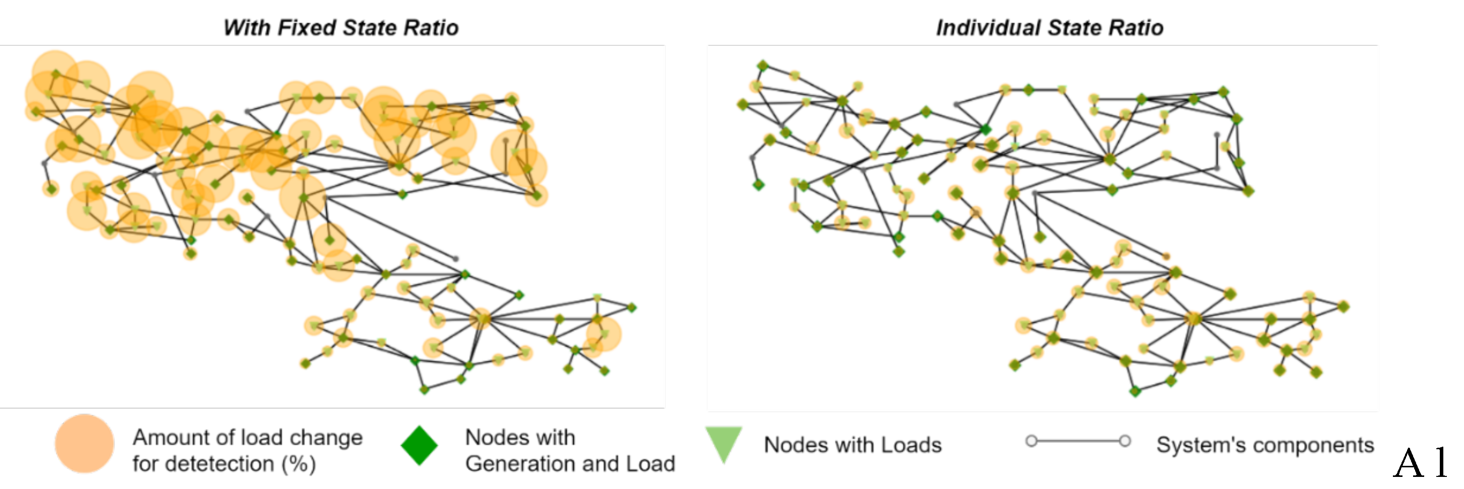
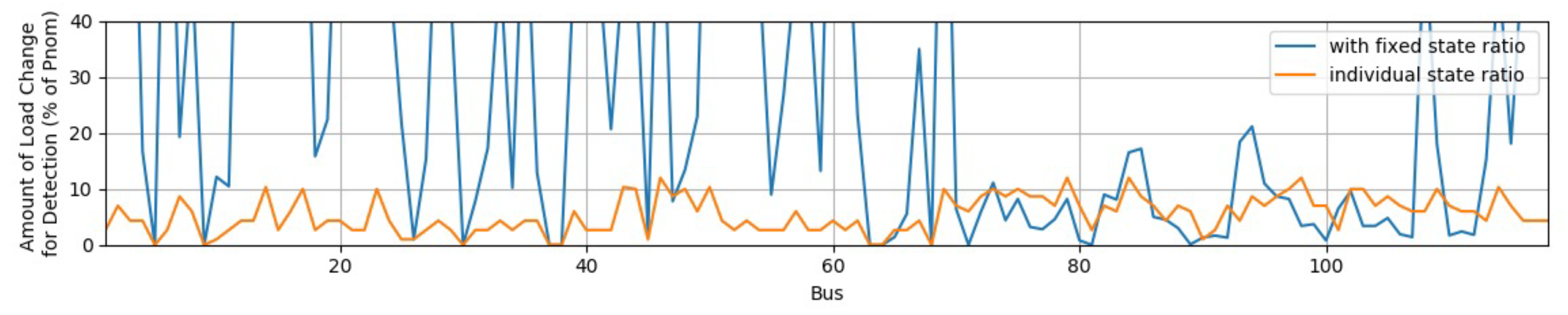
4.3. Effect of Process Noise and Anomalies Size

This case study considered the reference load flow scenario of the IEEE 30 bus test system [1]. A random load variation was included with a uniform variation of 0.5% in all loads in this case. Still, a sudden load increase of 5.0% occurs from t = 40 s to t = 90 s at six specific nodes (#3, #4, #15, #19, #21, and #30). The state ratio in this test case was also assumed as 0.03% of the previous state variable value. Initially, different levels and locations of gross errors were inserted in the simulations. Different levels of gross errors were added in different measurements during the simulations. Figure 9 illustrates the normalized innovation and the asymmetry index for this simulation. It shows that anomaly discrimination, based on the asymmetry index and the innovation level, enables an automatic suppression of different levels and locations of gross errors. An estimation accuracy like the previous section was obtained.

This second test also evaluated different sizes of sudden load changes and the detection by the asymmetry index of such change on the stationarity level. Different values of additional loads were included to the same six nodes (#3, #4, #15, #19, #21, and #30), that comprise 20% of the total net load.

Table 1. Dynamic State Estimator anomaly discrimination during different levels of sudden load change for the IEEE30 system with different state ratios for the state covariance matrix.

State Ratio	Discrimination Index	Sudden Load at Nodes: #3, #4, #15, #19 and #30
($\mathit{\alpha }$)		1.00%	2.00%	3.00%	5.00%	10.00%
$\alpha$ = 0.01%	Max.Norm.Innovation	2.2395	2.5890	2.9669	7.0648	14.7944
	Asymmetry Index	−0.7564	0.4354	0.2464	0.1318	0.1314
$\alpha$ = 0.1%	Max.Norm.Innovation	2.2472	1.6949	1.6857	3.1396	6.1013
	Asymmetry Index	−1.5551	0.5288	0.4443	0.6452	0.4482
$\alpha$ = 1.0%	Max.Norm.Innovation	2.2165	1.3483	1.3367	2.0801	3.2864
	Asymmetry Index	−1.6005	0.5130	−0.0642	0.5933	1.0896

presents the anomaly discrimination indexes, the maximum normalized innovation, and the asymmetry index, for each level of sudden load change, and different percentages for the state ratio. The method’s ability to detect such changes on the stationarity level depends on the assumed state covariance values. For instance, the state covariance matrix increase pushes the performance of the dynamic state estimator towards the static state estimator. Thereby, it becomes insensitive to changes on the stationarity level and neglects the additional information from the state-space model. It is noteworthy that the asymmetry index kept inside the accepted variation during such sudden load increases, i.e., it kept its value below the threshold value of 2.0.

Finally, different levels of random load variation were also evaluated.

Table 2. Mean absolute error of the estimation for different levels of load variation for the IEEE30 system with different state ratios for the state covariance matrix.

Load Variation	Maximum State Ratio in the State Covariance Matrix
	$\mathit{\alpha }$ = 0.00%	$\mathit{\alpha }$ = 0.01%	$\mathit{\alpha }$ = 0.1%	$\mathit{\alpha }$ = 1.0%	$\mathit{\alpha }$ = 10.0%
0.00%	8.9252 × 10−6	2.6840 × 10−5	7.9222 × 10−5	1.8912 × 10−4	2.3610 × 10−4
0.50%	4.4572 × 10−4	2.9600 × 10−4	2.1010 × 10−4	1.9453 × 10−4	2.3684 × 10−4
1.00%	12.1285 × 10−4	5.8336 × 10−4	3.7315 × 10−4	2.0537 × 10−4	2.3761 × 10−4
2.00%	61.1972 × 10−4	11.6417 × 10−4	7.1472 × 10−4	2.3882 × 10−4	2.3922 × 10−4

shows the mean absolute error, among all state variables, for different load variation levels and different percentages of state ratios

As can be seen, the DSE increases its performance under stationary conditions. Such performance is directly related to proper covariance matrix tuning. Besides, by increasing such covariance, the estimation reaches an error plateau given by a static state estimator’s performance. It is noteworthy that load variations of 2.0% are very large for the time span of the SCADA sampling rate, a few seconds. Such size of load change is more prone to be associated with sudden changes type of anomaly.

4.4. Effect of Different System Anomalies

To further explore and illustrate the asymmetry index, this simulation considers the IEEE 118 test system, a medium-size transmission system [27]. The simulation comprises one hundred sequential seconds, with the inclusion of 0.1% of random load variation in all nodes. This test scenario also considers a loss of generation at node #100, reducing 252 MW (6.1% of net load) at t = 40 s. The state ratio in this test case was assumed as 1.0% of the previous state variable value. Figure 10 illustrates the normalized innovation and the asymmetry index, demonstrating the automatic suppression of both gross errors and sudden changes while keeping accuracy throughout the estimation.

Figure 11 illustrates the cumulative probability plot of the normalized innovation for this test during different anomalies. It clearly shows the asymmetry present in the normalized innovation sample in the presence of gross errors, captured by the proposed anomaly discrimination strategy. Despite the results during the initial stationary event, as well as during the loss of generation, show a heavy-tailed distribution, it has more symmetry when compared to the presence of gross errors.

To demonstrate the effect of tuning and the influence of the sensitivity of the state variables, different levels of sudden load changes in individual buses were included across the power system. Two different approaches for tuning the state covariance matrix were evaluated, the first with a constant percentage of possible state variation, as in the previous simulations, and the second by choosing individual values of the state ratio parameter for each state variable. This later choice seeks to capture a more sensitive detection for anomalies that may occur in different parts of the system according to the respective state sensitivity.

Figure 12 illustrates a map with the detection level of sudden load change required to trigger the anomaly detection method in these two tuning approaches. The results are also present in Figure 13 with the obtained load change detection levels in each bus of the system. As it can be seen, the sensitivity of buses with less load requires larger levels of sudden changes, sometimes much more than 40%, to be captured by the anomaly detection method. However, as shown in the second simulation, by changing the tuning strategy for the state covariance was possible to increase such sensitivity accurately detect individual load changes less than 10% in most of the buses. Thus, showing the covariance matrix tuning as an important aspect of dynamic state estimators and their response against different anomalies.

4.5. Computational Aspects

Finally, the computational aspects of the previous simulations are presented in

Table 3. Mean processing time for different stages of the proposed DSE.

Test System	Prediction Step	Estimation Step	Anomaly Discrimination
IEEE14	<1.0 ms	<1.0 ms	1.9 ms
IEEE30	<1.0 ms	16.0 ms	9.7 ms
IEEE118	15.2 ms	360.0 ms	18.4 ms

. The tests were performed using a microcomputer with a Core i7 3.60 GHz, 16GB RAM with C programming language. The computational times only indicate the algorithm feasibility, and there is a large space for improvements, such as exploring sparsity treatments, improving data structures, and employing parallel computing techniques.

5. Conclusions

This paper presented a family of Kalman filter modeling for the power system dynamic state estimation problem. The presented formulation encompasses different piecewise stationary levels by discriminating different anomalies in the power system, such as gross errors or sudden load changes. The presented method automatically adapts itself to surpass the harmful effects of such anomalies while maintaining accuracy. Simulation results in IEEE transmission systems demonstrate the performance under dynamic anomalies, like different scenarios of gross errors, load ramps, sudden load changes, and generator contingency. Incorporating a dynamic perspective into the state estimation enables a sensible improvement on estimation accuracy when the system keeps a stationary level. Besides, by incorporating the asymmetry index into the innovation analysis, it is possible to track significant changes in the system’s dynamics accurately and adapt the estimator response. The state covariance tuning significantly impacts the Kalman filter performance, pushing its results between the static estimator and a smooth function. Future works comprise new Kalman filter tuning strategies based on power flow sensitivity, exploring the effects of bias into the state-space, and enhancing computational performance.

References

1. Bretas, A.S.; Bretas, N.G.; London, J.B.; Carvalho, B.E. Cyber-Physical Power Systems State Estimation; Elsevier: Amsterdam, The Netherlands, 2021. [Google Scholar]
2. Bretas, A.S.; Bretas, N.G.; Carvalho, B.; Baeyens, E.; Khargonekar, P.P. Smart grids cyber-physical security as a malicious data attack: An innovation approach. Electr. Power Syst. Res. 2017, 149, 210–219. [Google Scholar] [CrossRef]
3. Zhao, J.; Netto, M.; Huang, Z.; Yu, S.S.; Gomez-Exposito, A.; Wang, S.; Kamwa, I.; Akhlaghi, S.; Mili, L.; Terzija, V.; et al. Roles of dynamic state estimation in power system modeling, monitoring and operation. IEEE Trans. Power Syst. 2020, 36, 2462–2472. [Google Scholar] [CrossRef]
4. Rodriguez Paz, M.; Ferraz, R.; Bretas, A.S.; Leborgne, R. System unbalance and fault impedance effect on faulted distribution networks. Comput. Math. Appl. 2010, 60, 1105–1114. [Google Scholar] [CrossRef] [Green Version]
5. Zhao, J.; Gómez-Expósito, A.; Netto, M.; Mili, L.; Abur, A.; Terzija, V.; Kamwa, I.; Pal, B.; Singh, A.K.; Qi, J.; et al. Power system dynamic state estimation: Motivations, definitions, methodologies, and future work. IEEE Trans. Power Syst. 2019, 34, 3188–3198. [Google Scholar] [CrossRef]
6. Kalman, R.E. A new approach to linear filtering and prediction problems. Trans. ASME—J. Basic Eng. 1960, 35–45. [Google Scholar] [CrossRef] [Green Version]
7. Debs, A.S.; Larson, R.E. A dynamic estimator for tracking the state of a power system. IEEE Trans. Power Appar. Syst. 1970, 89, 1670–1678. [Google Scholar] [CrossRef]
8. Schweppe, F.; Masiello, R. A tracking static state estimator. IEEE Trans. Power Appar. Syst. 1971, 90, 1025–1033. [Google Scholar] [CrossRef]
9. Nishiya, K.; Hasegawa, J.; Koike, T. Dynamic state estimation including anomaly detection and identification for power systems. Proc. IEEE 1982, 129, 192–198. [Google Scholar] [CrossRef]
10. Falcao, D.; Cooke, P.; Brameller, A. Power system tracking state estimation and bad data processing. IEEE Trans. Power Appar. Syst. 1982, PAS-101, 325–333. [Google Scholar] [CrossRef]
11. Bretas, N. An iterative dynamic state estimation and bad data processing. Int. J. Electr. Power Energy Syst. 1989, 11, 70–74. [Google Scholar] [CrossRef]
12. Rousseaux, P.; Van Cutsem, T.; Liacco, T.D. Whither dynamic state estimation? Int. J. Electr. Power Energy Syst. 1990, 12, 104–116. [Google Scholar] [CrossRef]
13. Sarri, S.; Zanni, L.; Popovic, M.; Le Boudec, J.Y.; Paolone, M. Performance assessment of linear state estimators using synchrophasor measurements. IEEE Trans. Instrum. Meas. 2016, 65, 535–548. [Google Scholar] [CrossRef]
14. Fan, L.; Wehbe, Y. Extended Kalman filtering based real-time dynamic state and parameter estimation using PMU data. Electr. Power Syst. Res. 2013, 103, 168–177. [Google Scholar] [CrossRef]
15. Valverde, G.; Terzija, V. Unscented Kalman filter for power system dynamic state estimation. IET Gener. Transm. Distrib. 2010, 5, 29–37. [Google Scholar] [CrossRef]
16. Sharma, A.; Srivastava, S.C.; Chakrabarti, S. A cubature Kalman filter based power system dynamic state estimator. IEEE Trans. Instrum. Meas. 2017, 66, 2036–2045. [Google Scholar] [CrossRef]
17. Massignan, J.A.; London, J.B.; Miranda, V. Tracking Power System State Evolution with Maximum-correntropy-based Extended Kalman Filter. J. Mod. Power Syst. Clean Energy 2020, 8, 616–626. [Google Scholar] [CrossRef]
18. Zhou, N.; Meng, D.; Huang, Z.; Welch, G. Dynamic state estimation of a synchronous machine using PMU data: A comparative study. IEEE Trans. Smart Grid 2014, 6, 450–460. [Google Scholar] [CrossRef]
19. Do Coutto Filho, M.B.; De Souza, J.C.S.; Guimaraens, M.A.R. Enhanced bad data processing by phasor-aided state estimation. IEEE Trans. Power Syst. 2014, 29, 2200–2209. [Google Scholar] [CrossRef]
20. Durgaprasad, G.; Thakur, S. Robust dynamic state estimation of power systems based on M-estimation and realistic modeling of system dynamics. IEEE Trans. Power Syst. 1998, 13, 1331–1336. [Google Scholar] [CrossRef]
21. Zhao, J.; Mili, L. A framework for robust hybrid state estimation with unknown measurement noise statistics. IEEE Trans. Ind. Inform. 2017, 14, 1866–1875. [Google Scholar] [CrossRef]
22. Rouhani, A.; Abur, A. Linear phasor estimator assisted dynamic state estimation. IEEE Trans. Smart Grid 2016, 9, 211–219. [Google Scholar] [CrossRef]
23. Zhao, J. Dynamic State Estimation With Model Uncertainties Using H Extended Kalman Filter. IEEE Trans. Power Syst. 2017, 33, 1099–1100. [Google Scholar] [CrossRef]
24. Wang, Y.; Sun, Y.; Dinavahi, V.; Cao, S.; Hou, D. Adaptive robust cubature Kalman filter for power system dynamic state estimation against outliers. IEEE Access 2019, 7, 105872–105881. [Google Scholar] [CrossRef]
25. Do Coutto Filho, M.B.; de Souza, J.C.S. Forecasting-aided state estimation—Part I: Panorama. IEEE Trans. Power Syst. 2009, 24, 1667–1677. [Google Scholar] [CrossRef]
26. Castillo, M.R.; London, J.B.; Bretas, N.G.; Lefebvre, S.; Prévost, J.; Lambert, B. Offline detection, identification, and correction of branch parameter errors based on several measurement snapshots. IEEE Trans. Power Syst. 2010, 26, 870–877. [Google Scholar] [CrossRef]
27. IEEE Transmission System Test Cases: IEEE14, IEEE30 and IEEE118. IEEE Test Systems. Available online: https://labs.ece.uw.edu/pstca/ (accessed on 15 August 2021).
Figure 1. Signal model with external input known.
Energies 14 06787 g001
Figure 2. Distribution function of the New Information: (a) Dashed line for Normal Distribution and Solid line for Sudden load change situation; (b) Measurement Gross Error case.
Energies 14 06787 g002
Figure 3. The 3-bus transmission system and respective measurement set for the simulation.
Energies 14 06787 g003
Figure 4. Example of estimated state variables (voltage magnitude and phase angle) at bus #2 during the simulations, with the dynamic state estimator and with a static state estimator.
Energies 14 06787 g004
Figure 5. The IEEE 14 bus transmission system and respective measurement set for the simulation.
Energies 14 06787 g005
Figure 6. Example of estimated state variables (voltage magnitude and phase angle) at bus 14 during the simulations with the adaptive dynamic state estimator.
Energies 14 06787 g006
Figure 7. Boxplot of estimation error in all state variables at each instant of the simulation: (a) conventional Kalman Filter; (b) proposed Adaptive Dynamic State Estimator.
Energies 14 06787 g007
Figure 8. Maximum normalized innovation and asymmetry index for the IEEE14 in the simulations.
Energies 14 06787 g008
Figure 9. Maximum normalized innovation and asymmetry index for the IEEE30 in the simulations.
Energies 14 06787 g009
Figure 10. Maximum normalized innovation and asymmetry index for the IEEE118 in the simulation.
Energies 14 06787 g010
Figure 11. Probability plots for the normalized innovation in different instants: (left) in a stationary condition; (middle) with multiple gross errors; (right) during a loss of generation event.
Energies 14 06787 g011
Figure 12. Locational aspect of sudden load change detection with two different state covariances tuning: the first with a fixed state ratio for all buses and the second with an individual level of state ratio for each bus.
Energies 14 06787 g012
Figure 13. Amount of load change, in the percentage of the nominal value, in each individual node, detected as an anomaly for two different state covariances tuning.
Energies 14 06787 g013