Optimal Determination Method of the Transposition Steps of An Extra-High Voltage Power Transmission Line

Abstract

During the design of extra-high-voltage transmission lines, studies of the influence of asymmetry due to the phase difference of the parameters on its processes and the electrical network were performed. To compensate for this source of asymmetry for transmission lines longer than 100 km, a relatively simple technical means was proposed and implemented—phase transposition (change of the mutual location of phase wires in space). However, at the same time transposition causes additional capital costs in construction and reduces reliability during operation, so when designing a specific transmission line, extra-high-voltage is desirable to evaluate the effectiveness of the use of this measure in the real electricity network. Thus, under certain conditions, even for a transmission line 600 km in length, it was possible to perform either an incomplete transposition cycle, or abandon this measure altogether.

1. Introduction

The main source of current unbalance and voltages in normal modes of operation of electrical systems is the phase-by-phase difference in electrical parameters of the line. Asymmetry parameters of overhead lines are a result of their design. Particular attention is paid to asymmetry issues when creating extra-high-voltage (EHV) and ultra-high-voltage (UHV) lines, since their length in some sections can reach 500–1000 km. Traditional lines carrying 500–1150 kV are used, as a rule, for single-circuit supports with horizontal phases. To limit the asymmetry of such kind of transposition is usually applied as a simple, reliable, and at the same time effective method [1,2,3,4,5,6,7,8,9,10]. Phase conductor transposition; i.e., cyclical change in their relative position, is symmetrical to the resulting longitudinal and transverse resistance of the line as a whole. The balancing of the line parameters can also be carried out by constructive measures by increasing the height of the suspension of the middle phase in comparison with the extreme phases; i.e., with triangular phase arrangement.

The simplest, most reliable, and effective means of reducing the unbalance of currents and voltages is line phase transposition. Enough details of the transposition of three-phase air lines! EHV lines for long distances were considered in [1,2,3,4,5,6,7,8,9,10]. However, the choice and justification of transposition schemes remains relevant for nontraditional lines, such as three-phase lines with a backup phase, or four-phase, keeping in mind not only long-distance, but also ultra-long lines. The need for a more thorough consideration of the issues of transposition is also associated with a circumstance to which scientists first drew attention [11,12,13,14,15]. The point is that when considering the conditions for the implementation of SPAR in EHV and UHV lines, it is necessary to take into account the real line transposition, since it has a noticeable effect on the magnitude of the feed arc currents. Moreover, it can be assumed that the transposition of the line is a necessary condition, without which it is not possible to ensure a successful single-phase auto-reclose in the EHV and UHV lines when using the simplest method based on the inclusion of zero reactors in the neutral shunt reactors.

The dissimilarity of the parameters of the phases of high-voltage overhead lines (longitudinal resistances and transverse conductivities) is the reason for the asymmetry of currents and voltages in the electrical network. Unbalance is mainly determined by negative sequence current and voltage. The most significant factor characterizing the permissible value of current unbalance is the condition for reliable operation of relay protection. To reduce the asymmetry of currents and voltages during this mode, transposition of phase wires of overhead line is performed. Known three-phase overhead power lines, along the phase wires of which high-frequency (HF) are organized channels of information transmission and the permissible asymmetry, cannot be ensured by performing one ideal cycle of phase transposition. In this case, an ideal transposition cycle is understood as a cycle with equal step lengths.

Disadvantages are eliminated in a three-phase high-voltage overhead lines, in which, in order to reduce asymmetry on the line under consideration, several ideal transposition cycles are performed, However, each transposition support of overhead lines is a weak point, complicates the performance of preventive tests and repair work, and also reduces the reliability of the line as a whole and causes a complication of the design of the supports and an increase in the number of insulator strings and the total weight of the supports. In addition, the transposition of the phases has a significant influence on the characteristics of attenuation and unevenness of the HF linear path [4,5].

Asymmetry in the electrical network is mainly determined by the reverse sequence, as noted in [12]. Therefore, in the future we limit ourselves to the analysis of the asymmetry coefficients for the reverse sequence voltage. As indicated in [16,17,18,19,20,21,22,23,24,25], the maximum allowable asymmetry in the reverse sequence voltage is 2%. It is recommended to take the given values of permissible asymmetry for a specific OHL with a margin, taking into account the fact that complete asymmetry consists of the influence of all lines coming to the substation, as well as other possible sources of asymmetry, in particular asymmetric loading.

The worst case in terms of phase-by-phase difference of EHV parameters is an untransposed line, but it should be noted that as can be seen from Figure 1, the values of phase-by-phase asymmetry do not exceed the maximum allowable value in the case of line lengths up to 180 km. Application of incomplete transposition cycle Figure 2 is possible for line lengths up to 280 km under condition $k_{u2}\le 2,\%$. A simplified transposition scheme can be applied to a line up to 460 km long under asymmetry.

2. Methodology of Determination Optimal Steps of Scheme Transposition

Nevertheless, the leased information transmission channels in several cases do not meet the requirements for emergency automation and relay protection channels, and in addition, the lease of information transmission channels requires significant annual costs. The invention aims to improve the reliability and effectiveness of overhead lines by reducing the line current unbalance. This goal is achieved by the fact that in the known three-phase high voltage overhead power lines, consisting of sections with supports of various designs and containing three transposition steps, numbered from the beginning to the end of the line, the length of the first transposition step is taken equal to:

$$x_1=l\frac{{\alpha }_2{\beta }_2-{\alpha }_3{\beta }_2}{{\alpha }_1({\beta }_2-{\beta }_3)+{\alpha }_2({\beta }_3-{\beta }_1)+{\alpha }_3({\beta }_1-{\beta }_2)}$$

(1)

and the second transposition step is taken equal to:

$$x_2=l\frac{{\alpha }_3{\beta }_1-{\alpha }_1{\beta }_2}{{\alpha }_1({\beta }_2-{\beta }_3)+{\alpha }_2({\beta }_3-{\beta }_1)+{\alpha }_3({\beta }_1-{\beta }_2)}$$

(2)

where ${\alpha }_1=Re(\frac{{\displaystyle \sum _m{Z}_{m1}{l}_{m1}{k}_{m1}}}{x_1^1}),{\alpha }_2=Im(\frac{{\displaystyle \sum _m{Z}_{m1}{l}_{m1}{k}_{m1}}}{x_1^1})$; $Z_{m1}$ is specific mutual longitudinal resistance in the diagrams of the reverse and direct sequences of the section of the line’s m-th structure at the transposition step $x_1^1$; $l_{m1}$ is the length of the section of the m-th construction line at the transposition step; overhead line length $l$ is a coefficient taking into account the distribution of resistance $Z_{m1}$ in the U-shaped negative sequence the section of the structure line at the transposition step $x_1^1$; $x_1^1$ is the length of the first step of the transposition in the first approximation, determined by Formulas (1) and (2), in which, instead of ${\alpha }_1$ and ${\beta }_1$, respectively, are substituted and equal:

$$a_1=Re(\frac{{\displaystyle \sum _m{Z}_{m1}^1{l}_{m1}^1{k}_{m1}^1}}{l/3}),b_1=Im(\frac{{\displaystyle \sum _m{Z}_{m1}^1{l}_{m1}^1{k}_{m1}^1}}{l/3})$$

(3)

where $Z_{m1}^1{l}_{m1}^1{k}_{m1}^1$ are the same, respectively, for transposition steps with lengths 1/3.

For known three-phase overhead power lines of high voltage, their permissible asymmetry cannot be ensured by performing one ideal cycle of transposition [26,27,28,29,30,31,32,33,34,35].

In this case, either the relay protection is roughened up and the performance of the HF channels is preserved, or several ideal cycles of phase transposition are performed, while the requirement for detuning the relay protection (RP) is satisfied, but there is no way to organize reliable HF channels [32,33,34,35,36,37,38,39,40].

The proposed technical solution, unlike the known ones, ensures simultaneous reliability of the functioning of relay protection and high-frequency communication under consideration, which is especially important for the smooth operation of intersystem communication lines.

Due to the difference in the parameters of the phases of high-voltage overhead lines, as a rule, it is carried out according to the method according to which the asymmetry introduced by the line in the scheme of the reverse sequence is characterized by longitudinal electromagnetic force (EMF):

$${\stackrel{•}{E}}^{(2)}=-{\stackrel{•}{I}}^{(2)}{\stackrel{•}{z}}^{(21)}$$

or taking into account ${\stackrel{•}{z}}^{(21)}={\displaystyle \sum _l{Z}_1^l}{X}_1^l$.

$${\stackrel{•}{E}}^{(21)}=-j^{(-1)}{\displaystyle \sum _l{Z}_1^l}{X}_1^l$$

(4)

where $Z_1^l$ is the linear resistance determined by a well-known method, and the value $Z_1^l$ depends on the relative position of the phases and on the design OL.

Resistance of $Z_1^l$ on i-th step ideal cycle of transposition is determined by:

$$Z_1^1=\mathrm{Im}(\frac{{\displaystyle \sum _m{Z}_{m1}^1{l}_{m1}^1{k}_{m1}^1}}{l/3})$$

(5)

where the coefficient is determined by the equation:

$$k=\frac{1}{2}(1+\frac{Z_0^{(2)}{Y}_0^{(21)}}{Y_0^{(2)}{Z}_0^{(21)}})ch\sqrt{Z_0^{(2)}{Y}_0^{(2)}}+\frac{1}{2}(1-\frac{Z_0^{(2)}{Y}_0^{(21)}}{Y_0^{(2)}{Z}_0^{(21)}})\frac{sh\sqrt{Z_0^{(2)}{Y}_0^{(2)}}}{Z_0^{(2)}{Y}_0^{(2)}}$$

(6)

and $Z_0^{(2)},Y_0^{(2)},Z_0^{(21)},Y_0^{(21)}$ are determined by method [1,2,3,4,5].

Thus, the equivalent circuit of the overhead line is represented in the form of a cascade connection of U-shaped links of sections that are homogeneous in design. Then Expression (4), taking into account (5), takes the form:

$$E^{(2)}=-I^{(1)}{\displaystyle \sum _l(\frac{{\displaystyle \sum _m{Z}_{m1}^1{l}_{m1}^1{k}_{m1}^1}}{l/3})}$$

(7)

The minimum condition of the current’s reverse sequence in the line will be:

$$f={\displaystyle \sum _l(\frac{{\displaystyle \sum _m{Z}_{m1}^1{l}_{m1}^1{k}_{m1}^1}}{l/3})}{x}_1^1=\min$$

(8)

where, for implementation of this condition, verified magnitudes are $x_1^1$.

The lengths of the sections into which the line is divided by transposition supports are determined by the location of these supports. Two transposition supports divide the overhead line into three sections with lengths $x_1^1$, $x_2^1$, $x_3^1$; i.e.:

$$l={\displaystyle \sum _{l=1}^3{x}_1^1}$$

Magnitudes $x_1^1$ will correspond to extreme functions at conditions:

$$\frac{\partial f}{\partial x_1^l}=0;\frac{\partial f}{\partial x_2^l}=0;\frac{\partial f}{\partial x_n^l}=0$$

At installation 2, transposition towers with account, $x_3^l=l{x}_1^l-x_2^l$:

$$\begin{array}{l}\frac{\partial f}{\partial x_1^l}=2[(a_1-a_3)x_1^l+(a_2-a_3)x_2^l+a_{3}l]\times \\ \times (a_1-a_3)+2[(b_1-b_3)x_1^l+(b_2-b_3)x_2^l+b_{3}l(b_1-b_3)=0\end{array}$$

(9)

$$\begin{array}{l}\frac{\partial f}{\partial x_2^l}=2[(a_1-a_3)x_1^l+(a_2-a_3)x_2^l+a_{3}l]\times \\ \times (a_2-a_3)+2[(b_1-b_3)x_1^l+(b_2-b_3)x_2^l+b_{3}l(b_2-b_3)=0\end{array}$$

(10)

where

$$\begin{array}{l}{\alpha }_1=\mathrm{Re}(\frac{{\displaystyle \sum _m{Z}_{m1}{l}_{m1}{k}_{m1}}}{x_1^1})\\ {\alpha }_1=\mathrm{Im}(\frac{{\displaystyle \sum _m{Z}_{m1}{l}_{m1}{k}_{m1}}}{x_1^1})\end{array}$$

(11)

After transformations (9) and (10), we get:

$$\begin{array}{l}[{(a_1-a_3)}^2+{(b_1-b_3)}^2]x_1^l+[(a_2-a_3)(a_1-a_3)+\\ +(b_2-b_3)(b_1-b_3)x_2^l=-[a_3(a_1-a_3)+b_3(b_1-b_3)]l\end{array}$$

(12)

$$\begin{array}{l}[{(a_1-a_3)}^2(a_2-a_3)]+[(b_1-b_3)(b^2-b^3)x_1^l+\\ +[{(a_2-a_3)}^2+{(b_2-b_3)}^2]x_2^l=-[a_3(a_2-a_3)+b_3(b_2-b_3)]l\end{array}$$

(13)

Equations (12) and (13) will be:

$$\begin{array}{l}A{x}_1^l+B{x}_2^l=C\\ B{x}_1^l+D{x}_2^l=C\end{array}$$

(14)

The solution of which, in accordance with Cramer’s rule, will be:

$$\begin{array}{l}{x}_1^l=\frac{{\Delta }_1}{\Delta }\\ x_2^l=\frac{{\Delta }_2}{\Delta }\end{array}$$

where

$$\begin{gathered} \Delta =\left|\begin{array}{cc}A& B\\ B& D\end{array}\right|=AD-B^2 \\ {\Delta }_1=\left|\begin{array}{cc}C& B\\ E& D\end{array}\right|=CD-BE \\ {\Delta }_2=\left|\begin{array}{cc}A& C\\ B& E\end{array}\right|=AE-BC \end{gathered}$$

After performing further transformations, we obtain a formula for determining $x_1^l$ and $x_2^l$:

$$x_1^l=l\frac{a_2{b}_3-a_3{b}_2}{a_1(b_2-b_3)+a_2(b_3-b_1)+a_3(b_1-b_2)}$$

(15)

$$x_2^l=l\frac{a_3{b}_1-a_1{b}_3}{a_1(b_2-b_3)+a_2(b_3-b_1)+a_3(b_1-b_2)}$$

(16)

To determine the nature of the extreme at the obtained values $x_1^l$ and $x_2^l$, we determine the sign of the second derivative of the function f:

$$\begin{gathered} \frac{{\partial }^{2}f}{{(\partial x_1^l)}^2}={(a_1-a_3)}^2+{(b_1-b_3)}^2>0 \\ \frac{{\partial }^{2}f}{{(\partial x_2^l)}^2}={(a_2-a_3)}^2+{(b_2-b_3)}^2>0 \end{gathered}$$

(17)

Since the second derivatives are positive, the considered function $f$ for the obtained values $x_1^l$ and $x_2^l$ are minimum.

Taking into account the real structure of overhead lines $x_1^l$ at different lengths of transposition steps is performed by replacing the length of the ideal step l/3 with the length of the real step in Expression (12) for determination, as a result of which we respectively obtain ${\alpha }_1$ and ${\beta }_1$ (3).

Thus, the lengths of the steps of the transposition x₁ and x₂ are also determined by Formulas (1) and (2).

3. Comparison of Transposition Schemes According to the Condition of the Minimum Level of Asymmetry

A 330 kV overhead line with a length of 600 km in a section 400 km long, starting from the beginning of the line, is placed on portal supports with a horizontal arrangement of phase wires (support type 1), and for the next 200 km it is made into one circuit on a double-circuit single-column support with a triangular arrangement of wires (the second the chain is used for another transmission) (support type 2). The design of both types of supports is given in [1]. Specific resistance 2 (for different types of supports with different phase alternation) of a three-phase overhead line is determined according to the information given in

Table 1. The values of the parameters of the power transmission line depending on the phasing and the geometric arrangement of the phase wires on the tower.

Phase Sequence of a Three-Phase Overhead Line on a Tower			$\mathbf{Resistance}, {\mathit{Z}}_{\mathit{m}1}^{}[\mathit{O}\mathit{h}\mathit{m}\mathit{s}/\mathit{k}\mathit{m}]$
Horizontal Phase (Support Type 1)		Triangular Phase Arrangement (Type 2 Support)	With Support Type 1		With Support Type II
1	A B C	4	Ao		$0.0154\angle -{150}^{\circ }$
	O O O		Bo	$0.0292\angle -{150}^{\circ }$
			Co
2	C A B	5	Co	$0.0292\angle {90}^{\circ }$	$0.0154\angle {90}^{\circ }$
	O O O		Ao
			Bo
3	B C A	6	Bo	$0.0292\angle {30}^{\circ }$	$0.0154\angle -{30}^{\circ }$
	O O 0		Co
			Ao

. The values of the coefficient k for 330 kV overhead lines of various lengths are given in

Table 2. Coefficient $k$ change values depending on the line length.

$\mathit{l}[\mathit{k}\mathit{m}]$	100	200	300	400	500	600
$k$	0.997	0.989	0.975	0.957	0.933	0.904

.

The overhead line negative sequence current is determined by the formula:

$$I^{(2)}=\left|\frac{E^{(2)}}{X_{\Sigma }^{(2)}}\right|=\left|\frac{I^{(1)}{\displaystyle \sum _l({\displaystyle \sum _m{z}_{m1}{l}_{m1}{k}_1)}}}{X_{\Sigma }^{(2)}}\right|$$

(18)

Or, in percentage to current $I^{(1)}$:

$$I^{(2)}\%=\left|\frac{{\displaystyle \sum _l({\displaystyle \sum _m{z}_{m1}{l}_{m1}{k}_1)}}}{X_{}^{(2)}}\right|{10}^2$$

(19)

where $X_{\Sigma }^{(2)}$ is the equivalent resistance of the overhead line and systems, and $k_j=k_1{k}_2\dots k_j$ j—number of element links in a cascade equivalent circuit of overhead lines).

For various schemes for performing the transposition of overhead lines $I^{(2)}\%$:

• One perfect cycle of transposition.
  Then, in accordance with Formula (18), $I^{(2)}\%=1.3\%$.
  The maximum allowable unbalance by $I^{(2)}$ when choosing the lengths of the transposition cycles is 0.7%. Therefore, in the case under consideration, several ideal transposition cycles should be performed.
• Two ideal cycles of transposition. Then, in accordance with Formula (18), $I^{(2)}\%=0.65\%$.
• Performing transposition in accordance with the proposed technical solution.

According to the Formula (11), taking into account the data in the

Table 3. The values of the line parameters at three equal steps of the full transposition cycle.

Transposition Step Number	1	2	3
Length, $l[km]$	200	200	200
Phase sequence on the support	1	2	6
Resistance, $Z_{m1}^{}\times {10}^{-2}[Ohms/km]$	$2.92\angle -{150}^{\circ }$	$2.92\angle {90}^{\circ }$	$1.54\angle -{30}^{\circ }$
Coefficient, kl	0.989	0.9892	0.9893

, we define the parameters $a_1$ and $b_1$:

$$a_1+j{b}_1=z_1^l{k}_j^l=(-2.501-j1.444){10}^{-2}$$

$$a_2+j{b}_2=z_2^l{k}_2^l=(j2.888){10}^{-2}$$

$$a_3+j{b}_3=z_3^l{k}_3^l=(1.319-j0.761){10}^{-2}$$

Then, in accordance with Equations (15) and (16), we get:

$$x_1^l=154\mathrm{km}, x_2^l=154\mathrm{km}$$

In this case, $x_3^l=l-x_1^l-x_2^l=292$ km.

Table 4. Line parameter values at six equal steps of the full transposition cycle.

Transposition Step Number	1	2	3	4	5	6
Length, $l[\mathrm{km}]$	100	100	100	100	100	100
Phase sequence on the support	1	2	3	1	5	6
Resistance, $Z_{m1}^{}\times {10}^{-2}[\mathrm{Ohms}/\mathrm{km}]$	$2.92\angle -{150}^{\circ }$	$2.92\angle {90}^{\circ }$	$1.54\angle -{30}^{\circ }$	$2.92\angle -{150}^{\circ }$	$1.54\angle {90}^{\circ }$	$1.54\angle -{30}^{\circ }$
Coefficient, kl	0.997	0.997 *	0.997	0.9974	0.9975	0.9976

shows the results for the case of an ideal transposition cycle when the line length is divided by 6 equal parts.

Obtained data are brought together in

Table 5. The values of the line parameters at the lengths of the transposition steps selected according to the developed method. Equations (15) and (16).

Transposition Step Number	1	2	3	4
Length, $l[\mathrm{km}]$	154	154	92	200
Phase sequence on the support	1	2	3	6
Resistance,$Z_{m1}^{}\times {10}^{-2}[\mathrm{Ohms}/\mathrm{km}]$	$2.92\angle -{150}^{\circ }$	$2.92\angle {90}^{\circ }$	$2.92\angle -{30}^{\circ }$	$1.54\angle -{30}^{\circ }$
Coefficient, kl	0.994	0.994	0.997	0.989

.

By Equation (3), and taking into account the data in Table 5, we obtained parameters ${\alpha }_1$ and ${\beta }_1$:

$${\alpha }_1+j{\beta }_1=(-2.514-j1.451){10}^{-2}$$

$${\alpha }_2+j{\beta }_2=(0+j2.902){10}^{-2}$$

$${\alpha }_3+j{\beta }_3=(1.698-j0.980){10}^{-2}$$

Obtained data are brought together in

Table 6. The values of the line parameters at the lengths of the transposition steps selected according to the developed method Equations (1) and (2).

Transposition Step Number	1	2	3	4
Length, $l[km]$	172	172	56	200
Phase sequence on the support	1	2	3	6
Resistance, $Z_{m1}^{}\times {10}^{-2}[Ohms/km]$	$2.92\angle -{150}^{\circ }$	$2.92\angle {90}^{\circ }$	$2.92\angle -{30}^{\circ }$	$1.54\angle -{30}^{\circ }$
Coefficient, kl	0.994	0.994	0.997	0.989

. Then, following Equation (18), $I^{(2)}\%=0.17\%$.

4. Estimation of the Influence of the Wire Transposition Scheme on the Parametric Optimization of the Operating Modes of the Main Electrical Networks

Usually, the development of parametric optimization methods is performed without taking into account the influence of the transposition scheme, and therefore without the influence of the phase-by-phase line unbalance. Taking into account the fact that a method was developed for determining the optimal steps of wire transposition, it is necessary to assess the degree of influence of phase-by-phase asymmetry in a transposition scheme with optimal steps on parametric optimization by using the criterion of active power losses. It should be noted that the transposition of the wires equalizes the longitudinal and transverse resistances and conductivity of the overhead power line.

As can be seen in the results in Table 4, Table 5 and Table 6, at the optimal steps of the transposition schemes, the levels of asymmetry were lower than at equal ones, in the case when the line was divided into six different sections. In the case of parametric optimization of the mode, it was necessary to understand whether it was necessary to take into account the wire transposition scheme and complicate the calculations. For this, it was necessary to develop a parametric optimization method with an ideal transposition cycle with equal steps and with optimal steps using the above method.

One of the measures to ensure the reduction of electricity losses was the optimization of the operating modes of EHV transmission lines in terms of voltage and reactive power. In this formulation, the problems of EHV transmission lines were considered in isolation for the three most common modes: minimum, maximum, and operational modes of power transmission. Analytical expressions for determining the loss of active power in the power line contain components of idling and short-circuit losses [41,42,43,44,45,46,47,48,49,50,51,52,53,54,55,56]. The latter are directly and inversely proportional, respectively, to the square of the voltage on the bus terminals, which determines the possibility of choosing the optimal voltage level. This provides a minimum amount of components of these losses.

The analysis of the modes of operation of the transmission line with controlled shunt reactors showed that in the case of CSR, there was a compensation of the charging power and regulation of the power flow. In this case, the loss of active power will be written as:

$$\begin{array}{l} \Delta P=\left[\begin{array}{l}\left(\frac{GR-(B+B_{reac})X}{2}+1\right)\left(2G^{2}R-2G(B+B_{reac})X+8G\right)+\\ +\frac{GX+(B+B_{reac})R}{2}\left(2G(B+B_{reac})R+2G^{2}X\right)\end{array}\right]U^2+\\ \left[\left(\frac{GR-(B+B_{reac})X}{2}+1\right)R+\frac{GX+(B+B_{reac})R}{2}X\right]\frac{P^2+Q^2}{U^2}-\\ 2P\left[\frac{{(GX+(B+B_{reac})R)}^2}{2}+R(2G^{2}R-2G(B+B_{reac})X+8G)\right]+\\ \left[2\left[X\left(2G^{2}R-2G(B+B_{reac})X+8G\right)-\left(\frac{GR-(B+B_{reac})X}{2}+1\right)\frac{GX+(B+B_{reac})R}{2}\right]\right]Q,[mW]\end{array}$$

(20)

where R—the active resistance, ohms; X—the inductive resistance, ohms; G—active conductivity, Cm; B—reactive conductivity, Sm; U—rated voltage, kV; P—active power, mW; and Q—reactive power, MVAr.

In turn, the voltage and reactive power depend on the number and composition of the line charging compensation devices. When regulating the mode of operation of the transmission line, it was necessary to minimize the power-loss function (20) by using independent mode parameters, which allowed us to obtain conditions for optimal regulation of reactive power flows of the transmission line, power CSR, and voltage at the connection point:

$$\frac{\partial \Delta P(Q,U,B_{reac})}{\partial U}=0,\frac{\partial \Delta P(Q,U,B_{reac})}{\partial B_{reac}}=0,\frac{\partial \Delta P(Q,U,B_{reac})}{\partial Q}=0$$

(21)

The analysis of active power losses $\Delta P$ with the established two groups of SR or CSR was carried out for the EHV transmission line with the following parameters: $l=400$ km—line length, $U=750$ kV—nominal line voltage, and wire phase design 4xAS-400/93. This was characterized by the following parameters: $r0=0.019$ ohm/km; $x0=0.289$ ohm/km; $g0=0.0325$ μS/km; and $b0=4.13$ μSm/km.

To analyze the power losses, a system of equations was compiled to find the optimal values of, $B_{reac}$, $Q$, and $U$:

$$\{\begin{array}{l}2U\left[\begin{array}{l}\left(\frac{GR-\left(B+B_{reac}\right)X}{2}+1\right)\left(2G^{2}R-2G\left(B+B_{reac}\right)X+8G\right)\\ +\frac{GX+\left(B+B_{reac}\right)R}{2}\left(2G\left(B+B_{reac}\right)R+2G^{2}X\right)\end{array}\right]-\\ \frac{2\left(P^2+Q^2\right)\left[R\left(\frac{GR-\left(B+B_{reac}\right)X+2}{2}\right)+X\left(\frac{\left(B+B_{reac}\right)R+GX}{2}\right)\right]}{U^3}=0\\ \left(\begin{array}{l}\frac{R\left(2X{G}^2+2\left(B+B_{reac}\right)RG\right)-X\left(8G+2G^{2}R-2\left(B+B_{reac}\right)GX\right)}{2}\\ +2GR\left(\frac{\left(B+B_{reac}\right)R+GX}{2}\right)-2GX\left(\frac{GR-\left(B+B_{reac}\right)X+2}{2}\right)\end{array}\right)U^2-\\ P\left[2R\left(\frac{\left(B+B_{reac}\right)R+GX}{2}\right)-4GRX\right]-Q\left[\begin{array}{l}4G{X}^2+R\left(\frac{GR-\left(B+B_{reac}\right)X+2}{2}\right)\\ -X\left(\frac{\left(B+B_{reac}\right)R+GX}{2}\right)\end{array}\right]=0\\ 2X(8G+2G^{2}R-2GX\left(B+B_{reac}\right)-2\left(\frac{R\left(B+B_{reac}\right)+GX}{2}\right)\left(\frac{GR-X\left(B+B_{reac}\right)+2}{2}\right)+\\ \frac{2Q\left[R\left(\frac{GR-X\left(B+B_{reac}\right)+2}{2}\right)+X\frac{R\left(B+B_{reac}\right)+GX}{2}\right]}{U^2}=0\end{array}$$

(22)

It should be noted that changes in the reactive power in the nodes led to changes in the node voltages of the network, in accordance with (22). The consequence of this, in turn, was a change in power losses in the network, as seen from (20). At the same time, changes in reactive power must correspond to the available range of regulation of sources and not cause unacceptable voltage deviations in the network nodes:

$$\begin{array}{l}{Q}_{\min }\le Q_i\le Q_{\max };\\ 0.95U_{}\le U_i\le 1.05U_{}\end{array}$$

(23)

To verify the obtained values $B_{reac}$, $Q$, and $U$, under the condition of the minimum of the function $\Delta P(Q,U,B_{reac})$, we first were required to find all partial derivatives of the 2nd order, calculate them at a point, and compose a Hesse matrix:

$$H=\left[\begin{array}{ccc}\frac{{\partial }^2\Delta P(B_{reac},U,Q)}{\partial B_{reac}{}^2}& \frac{\partial \Delta P(B_{reac},U,Q)}{\partial B_{reac}\partial Q}& \frac{\partial \Delta P(B_{reac},U,Q)}{\partial B_{reac}\partial U}\\ \frac{\partial \Delta P(B_{reac},U,Q)}{\partial Q\partial B_{reac}}& \frac{{\partial }^2\Delta P(B_{reac},U,Q)}{\partial Q^2}& \frac{\partial \Delta P(B_{reac},U,Q)}{\partial Q\partial U}\\ \frac{\partial \Delta P(B_{reac},U,Q)}{\partial U\partial B_{reac}}& \frac{\partial \Delta P(B_{reac},U,Q)}{\partial U\partial Q}& \frac{{\partial }^2\Delta P(B_{reac},U,Q)}{\partial U^2}\end{array}\right]$$

(24)

Conditions under which the angular minors of the Hesse matrix (24) satisfy the condition of the minimum of function (20) for the values $B_{reac}$, $Q$, $U$ are:

$${\delta }_1=\frac{{\partial }^2\Delta P(B_{reac},U,Q)}{\partial B_{reac}{}^2}>0$$

(25)

$${\delta }_2=\left|\begin{array}{cc}\frac{{\partial }^2\Delta P(B_{reac},U,Q)}{\partial B_{reac}{}^2}& \frac{\partial \Delta P(B_{reac},U,Q)}{\partial B_{reac}\partial Q}\\ \frac{\partial \Delta P(B_{reac},U,Q)}{\partial Q\partial B_{reac}}& \frac{{\partial }^2\Delta P(B_{reac},U,Q)}{\partial Q^2}\end{array}\right|>0$$

(26)

$${\delta }_3=\left|\begin{array}{ccc}\frac{{\partial }^2\Delta P(B_{reac},U,Q)}{\partial B_{reac}{}^2}& \frac{{\partial }^2\Delta P(B_{reac},U,Q)}{\partial B_{reac}\partial Q}& \frac{{\partial }^2\Delta P(B_{reac},U,Q)}{\partial B_{reac}\partial U}\\ \frac{{\partial }^2\Delta P(B_{reac},U,Q)}{\partial Q\partial B_{reac}}& \frac{{\partial }^2\Delta P(B_{reac},U,Q)}{\partial Q^2}& \frac{{\partial }^2\Delta P(B_{reac},U,Q)}{\partial Q\partial U}\\ \frac{{\partial }^2\Delta P(B_{reac},U,Q)}{\partial U\partial B_{reac}}& \frac{{\partial }^2\Delta P(B_{reac},U,Q)}{\partial U\partial Q}& \frac{{\partial }^2\Delta P(B_{reac},U,Q)}{\partial U^2}\end{array}\right|>0$$

(27)

When calculating the angular minors (23)–(25), the obtained optimal values $B_{reac}$, $Q$, and $U$, at which the minimum $\Delta P(Q,U,B_{reac})$ was reached, were checked.

For comparative analysis of the use of controlled and uncontrolled shunt reactors, a system of equations was developed to find the optimal values $Q$ and $U$ at a fixed value $B_{reac}$:

$$\hspace{0.33em}\left\{\begin{array}{l}\left(\begin{array}{l}\frac{R(2X{G}^2+2(B+B_{csr})RG)-X(8G+2G^{2}R-2(B+B_{csr})GX)}{2}\\ +2GR(\frac{(B+B_{csr})R+GX}{2})-2GX(\frac{GR-(B+B_{csr})X+2}{2})\end{array}\right)U^2-\\ P\left[2R(\frac{(B+B_{csr})R+GX}{2})-4GRX\right]-Q\left[\begin{array}{l}4G{X}^2+R(\frac{GR-(B+B_{csr})X+2}{2})\\ -X(\frac{(B+B_{csr})R+GX}{2})\end{array}\right]=0\\ 2X(8G+2G^{2}R-2GX(B+B_{csr})-2\left(\frac{R(B+B_{csr})+GX}{2}\right)\left(\frac{GR-X(B+B_{csr})+2}{2}\right)+\\ \frac{2Q\left[R\left(\frac{GR-X(B+B_{csr})+2}{2}\right)+X\frac{R(B+B_{csr})+GX}{2}\right]}{U^2}=0\end{array}\right.$$

(28)

To find $Q$ and $U$ using the system in Equation (28), the conductivity value $B_{reac}$ was changed discretely by switching off the group of single-phase shunt reactors. Installing uncontrolled SR also forms a Hesse matrix:

$$H=\left[\begin{array}{cc}\frac{{\partial }^2\Delta P(B_{reac},U,Q)}{\partial Q^2}& \frac{\partial \Delta P(B_{reac},U,Q)}{\partial Q\partial U}\\ \frac{\partial \Delta P(B_{reac},U,Q)}{\partial U\partial Q}& \frac{{\partial }^2\Delta P(B_{reac},U,Q)}{\partial U^2}\end{array}\right]$$

(29)

Conditions under which the angular minors of the Hesse matrix (29) satisfy the condition of minimum function (18) at values $Q$ and $U$ are:

$${\delta }_1=\frac{{\partial }^2\Delta P(B_{reac},U,Q)}{\partial Q^2}>0$$

(30)

$${\delta }_2=\left|\begin{array}{cc}\frac{{\partial }^2\Delta P(B_{reac},U,Q)}{\partial Q^2}& \frac{\partial \Delta P(B_{reac},U,Q)}{\partial Q\partial U}\\ \frac{\partial \Delta P(B_{reac},U,Q)}{\partial U\partial Q}& \frac{{\partial }^2\Delta P(B_{reac},U,Q)}{\partial U^2}\end{array}\right|>0$$

(31)

The obtained optimal $Q$ and $U$ values corresponded to the minimum of the function $\Delta P(Q,U)$.

Table 7. Results of parametric optimization when using CSR and SR for ideal transposed extra-high voltage power line.

Installation of SR				Installation of CSR
$B_{reac}$, Sm	$Q^{opt}$, MVAr	$U^{opt}$, kV	$\Delta P$, mWatt	$B_{reac}^{opt}$, Sm	$Q^{opt}$, MVAr	$U^{opt}$, kV	$\Delta P$, mWatt
−0.001066	−210	735	22.686	−0.0007	−180	768	20.908
−0.000533	−300	741	23.015

shows the obtained values for $Q^{opt}$ and $U^{opt}$, with the corresponding values in the case of installation of uncontrolled SR. For comparison, the optimal values of $B_{reac}$, $Q$, and $U$ are given in Table 7 and

Table 8. Results of parametric optimization when using CSR and SR for transposed extra-high voltage power lines by with optimal steps.

Installation of SR				Installation of CSR
$B_{reac}$, Sm	$Q^{opt}$, MVAr	$U^{opt}$, kV	$\Delta P$, mWatt	$B_{reac}^{opt}$, Sm	$Q^{opt}$, MVAr	$U^{opt}$, kV	$\Delta P$, mWatt
−0.001064	−208	732	22.456	−0.000691	−178	766	20.41
−0.00053	−297	739	22.98

for the case of an ideal transposition cycle with equal steps and with optimal steps appropriately, which corresponded to the minimum value of active power losses in the case of installation of CSR $\Delta P(Q,U,B_{reac})$. As can be seen from the data in this table, the optimal values of $U^{opt}$ corresponded to the available voltage control range (23).

For parametric optimization of the main electric network, the total losses of active power in the main electric network (Figure 2) of the nominal voltage of 750 kV are described by the expression:

$$\Delta P_{\Sigma }={\displaystyle \sum _{i\in 1}^n{\displaystyle \sum _{i\in 1j\ne 1}^n\Delta P_{ij}}}$$

(32)

where ΔP_ij—losses of active power of the transmission line, determined by Formula (18); and ij—substation numbers of the main electric network.

The equation of state of an equivalent quadrupole is:

$$\begin{array}{l}\left[\begin{array}{cc}{A}_{eq}& B_{eq}\\ C_{eq}& D_{eq}\end{array}\right]=\left[\begin{array}{cc}{A}_{L1}& B_{L1}\\ C_{L1}& D_{L1}\end{array}\right]\left[\begin{array}{cc}{A}_{csr1}& B_{csr1}\\ C_{csr1}& D_{csr1}\end{array}\right]\left[\begin{array}{cc}{A}_{L2}& B_{L2}\\ C_{L2}& D_{L2}\end{array}\right]\left[\begin{array}{cc}{A}_{csr2}& B_{csr2}\\ C_{csr2}& D_{csr2}\end{array}\right]\\ \times \left[\begin{array}{cc}{A}_{csr3}& B_{csr3}\\ C_{csr3}& D_{csr3}\end{array}\right]\left[\begin{array}{cc}{A}_{L3}& B_{L3}\\ C_{L3}& D_{L3}\end{array}\right]\left[\begin{array}{cc}{A}_{csr4}& B_{csr4}\\ C_{csr4}& D_{csr4}\end{array}\right]\left[\begin{array}{cc}{A}_{L4}& B_{L4}\\ C_{L4}& D_{L4}\end{array}\right]\end{array}$$

(33)

To determine the optimal values of $B_{reac}$, $Q$, and $U$, the same approach was used as for the parametric optimization of the EHV transmission line. In the case of the establishment of CSR approach, (22)–(27) were used; and for the uncontrolled SR approach, (28)–(31) were used. The results of the calculation of active power losses are summarized in

Table 9. Results of parametric optimization when using CSR and SR for bulk electrical power network with ideal transposed extra-high voltage power lines.

Installation of SR				Installation of CSR
$B_{reac}$, Sm	$Q^{opt}$, MVAr	$U^{opt}$, kV	$\Delta P$, mWatt	$B_{reac}^{opt}$, Sm	$Q^{opt}$, MVAr	$U^{opt}$, kV	$\Delta P$, mWatt
−0.002665	−210	735	165.005	−0.0001	−450	720	100,158
−0.002132	−100	744	147.58
−0.001599	187	731	135.47
−0.001066	268	748	127.58
−0.000533	115	741	120.015

and

Table 10. Results of parametric optimization when using CSR and SR for bulk electrical power network with extra-high voltage power lines with optimal transposition steps.

Installation of SR				Installation of CSR
$B_{reac}$, Sm	$Q^{opt}$, MVAr	$U^{opt}$, kV	$\Delta P$, mWatt	$B_{reac}^{opt}$, Sm	$Q^{opt}$, MVAr	$U^{opt}$, kV	$\Delta P$, mWatt
−0.002559	−208	732	163.01	−0.000097	−445	720	96,158
−0.002005	−105	741	147.05
−0.001399	167	735	131.47
−0.001105	255	752	124.18
−0.000505	113	745	118.02

for the case of an ideal transposition cycle with equal steps and with optimal steps appropriately, in case of installation of CSR at optimum values $Q^{opt}$, $U^{opt}$, and $B_{reac}^{opt}$. The results of calculations $Q^{opt}$ and $U^{opt}$ when installing SR with a discrete change of inductance are given in Table 10.

5. Conclusions

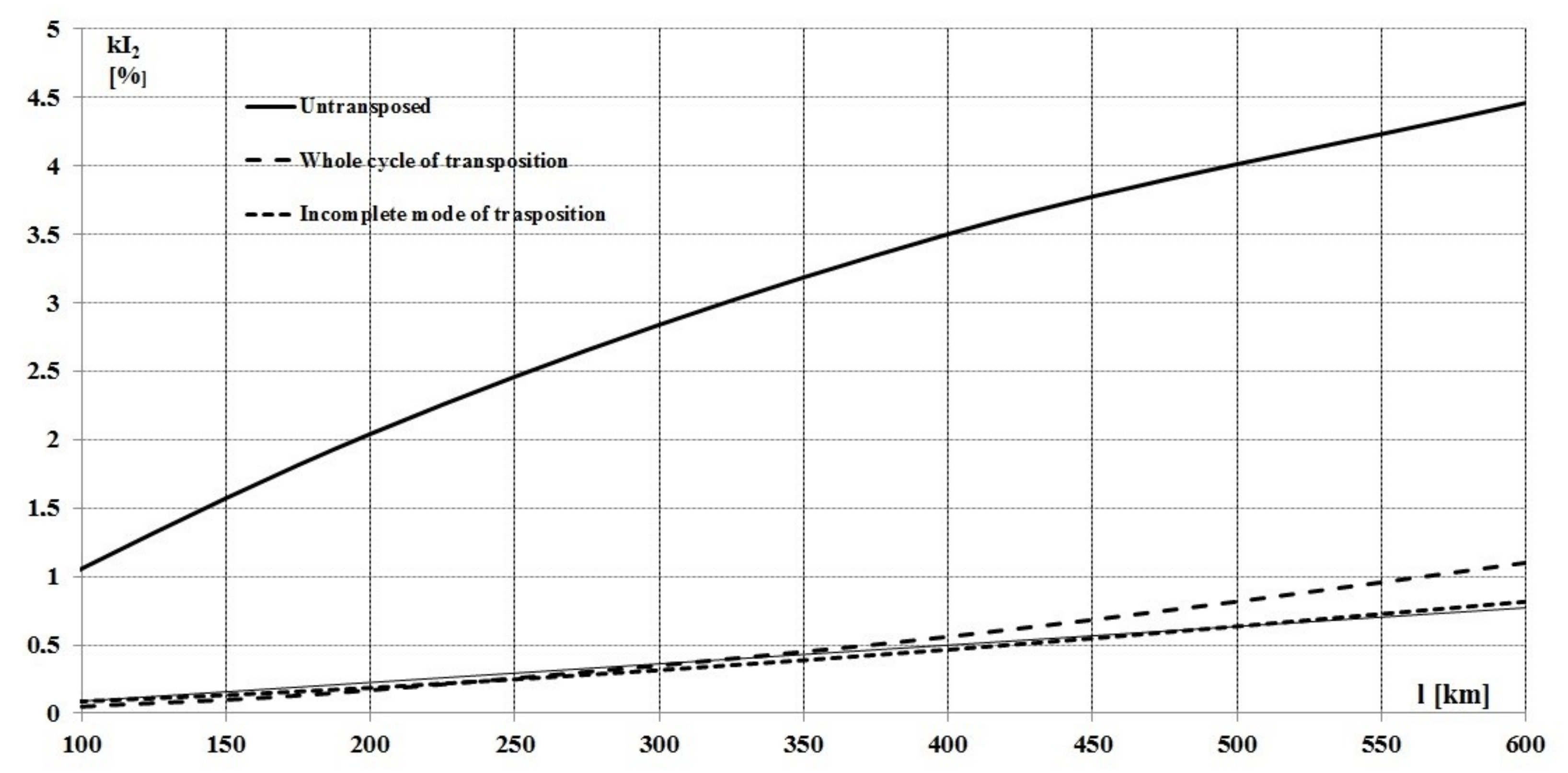
• As can be seen in Table 5 and Table 6, the levels of asymmetry for the incomplete transposition cycle did not significantly exceed the maximum allowable values for the lengths of lines. That is, with such a transposition scheme, the necessary levels of voltage asymmetry were provided, and it can be offered as a relatively inexpensive balancing measure, with a length of the EHV transmission line of more than 600 km. If the length of the transmission line exceeds 400 km, full transposition cycles must be used. In relation to the ideal scheme of transposed, the levels of asymmetry did not exceed the maximum allowable values.
• A method was proposed for determining the optimal steps of transposition based on operation in normal full-phase modes, as well as for carrying out planned phase-by-phase repairs with its full development. The optimal steps of the transposition cycles at which the permissible levels of asymmetry were achieved, which were 1% less than the ideal transposition cycle, were substantiated. This result, in contrast to the traditional scheme used, allowed optimal use of the same number of transposition supports and phase alternation of the line. It should be noted that the proposed transposition steps can increase the capacity of the transmission line by reducing the level of asymmetry. The criteria of optimal method determination is permissible levels of asymmetry.

References

1. Kundul, S.; Ghosh, T.; Maitra, K.; Acharjee, P.; Thakur, S.S. Optimal Location of SVC Considering Techno-Economic and Environmental Aspect. In Proceedings of the 2018 ICEPE 2nd International Conference on Power, Energy and Environment: Towards Smart Technology, Shillong, India, 1–2 June 2018; pp. 15–19. [Google Scholar] [CrossRef]
2. Gu, S.; Dang, J.; Tian, M.; Zhang, B. Compensation degree of controllable shunt reactor in EHV/UHV transmission line with series capacitor compensation considered. In Proceedings of the International Conference on Mechatronics, Control and Electronic Engineering (MCE 2014), Shenyang, China, 29–31 August 2014; pp. 65–68. [Google Scholar] [CrossRef] [Green Version]
3. Chandrasekhar, R.; Chatterjee, D.; Bhattarcharya, T. A Hybrid FACTS Topology for Reactive Power Support in High Voltage Transmission Systems. In Proceedings of the IECON 2018—44th Annual Conference of the IEEE Industrial Electronics Society, Washington, DC, USA, 21–23 October 2018; pp. 65–70. [Google Scholar] [CrossRef]
4. Bryantsev, A.M.; Bryantsev, M.A.; Bazylev, B.I.; Dyagileva, S.V.; Negryshev, A.A.; Karymov, R.; Makletsova, E.; Smolovik, S. Power compensators based on magnetically controlled shunt reactors in electric networks with a voltage between 110 kV and 500 kV. In Proceedings of the 2010 IEEE/PES Transmission and Distribution Conference and Exposition: Latin America (T&D-LA), Sao Paulo, Brazil, 8–10 November 2010; pp. 239–244. [Google Scholar]
5. Kuchanskyy, V.V. The prevention measure of resonance overvoltges in extra high voltage transmission lines. In Proceedings of the 2017 IEEE First Ukraine Conference on Electrical and Computer Engineering (UKRCON), Kyiv, Ukraine, 29 May–2 June 2017. [Google Scholar]
6. Kuchanskyy, V.V.; Zaitsev, I.O. Corona Discharge Power Losses Measurement Systems in Extra High Voltage Transmissions Lines. In Proceedings of the 2020 IEEE 7th International Conference on Energy Smart Systems (ESS), Kyiv, Ukraine, 12–14 May 2020; pp. 48–53. [Google Scholar] [CrossRef]
7. Kuchanskyy, V.; Malakhatka, D.; Blinov, I. Application of Reactive Power Compensation Devices for Increasing Efficiency of Bulk Electrical Power Systems. In Proceedings of the 2020 IEEE 7th International Conference on Energy Smart Systems (ESS), Kyiv, Ukraine, 12–14 May 2020; pp. 83–86. [Google Scholar] [CrossRef]
8. Kuchanskyy, V. Application of Controlled Shunt Reactors for Suppression Abnormal Resonance Overvoltages in Assymetric Modes. In Proceedings of the 2019 IEEE 6th International Conference on Energy Smart Systems (ESS), Kyiv, Ukraine, 17–19 April 2019; pp. 122–125. [Google Scholar] [CrossRef]
9. Tugay, Y.; Kuchanskyy, V.; Tugay, I. The Using of Controlled Devices for the Compensation of Charging Power on EHV Power Lines in Electric Networks. Tekh. Elektrodyn. 2021, 1, 053. [Google Scholar] [CrossRef]
10. Kuznetsov, V.; Tugay, Y.; Kuchanskyy, V. Overvoltages in open-phase mode. Tekh. Elektrodyn. 2012, 40–41. (In Ukrainian) [Google Scholar]
11. Kuznetsov, V.; Tugay, Y.; Kuchanskyy, V. Influence of corona discharge on the internal ovevoltages in highway electrical networks. Tekh. Elektrodyn. 2017, 55–60. (In Ukrainian) [Google Scholar] [CrossRef] [Green Version]
12. Kuchanskyy, V. Criteria of resonance overvoltages occurrence in abnormal conditions of extra high voltage transmission lines. Visnyk Nauk. Pr. Vinnytskoho Nastionalnoho Tekh. Univ. 2016, 51–54. [Google Scholar] [CrossRef] [Green Version]
13. Blinov, I.V.; Zaitsev, I.O.; Kuchanskyy, V.V. Problems, methods and means of monitoring power losses in overhead transmission lines. In Systems, Decision and Control in Energy I; Babak, V.P., Isaienko, V., Zaporozhets, A.O., Eds.; Springer: Berlin/Heidelberg, Germany, 2020; pp. 123–136. [Google Scholar]
14. Kuznetsov, V.G.; Tugay, Y.I.; Kuchansky, V.V.; Likhovid, Y.G.; Melnichuk, V.A. Resonant overvoltages in non-sinusoidal mode of the main electric network. Elektrotehn. Elektromeh. 2018, 69–73. (In Ukrainian) [Google Scholar] [CrossRef]
15. Hunko, I.; Kuchanskyi, V.; Nesterko, A.; Rubanenko, O. Modes of Electrical Systems and Grids with Renewable Energy Sources; LAMBERT Academic Publishing: Chisinau, Moldova, 2019; p. 184. ISBN 978-613-9-88956-3. [Google Scholar]
16. Kuchanskyy, V.; Rubanenko, O. Influence assesment of autotransformer remanent flux on resonance overvoltage. UPB Sci. Bull. Ser. C Electr. Eng. 2020, 82, 233–250. [Google Scholar]
17. Kuchanskyy, V.; Satyam, P.; Rubanenko, O.; Hunko, I. Measures and technical means for increasing efficiency and reliability of extra high voltage transmission lines. Przegląd Elektrotechniczny 2020, 2020, 135–141. [Google Scholar] [CrossRef]
18. Martinich, T.; Nagpal, M.; Manuel, S. Damaging Open-Phase Overvoltage Disturbance on a Shunt-Compensated 500-kV Line. IEEE Trans. Power Deliv. 2015, 30, 412–419. [Google Scholar]
19. Bollen, M.H.J. What is power quality? Review. Electr. Power Syst. Res. 2003, 66, 5–14. [Google Scholar] [CrossRef]
20. Wenjuan, Z.; Tolbert, L.M. Survey of reactive power planning methods. In Proceedings of the 2005 PES General Meeting, San Francisco, CA, USA, 16 June 2005; pp. 1430–1440. [Google Scholar]
21. Chengxi, L.; Nan, Q.; Bak, C.L.; Yini, X. A hybrid optimization method for reactive power and voltage control considering power loss minimization. In Proceedings of the 2015 IEEE Eindhoven PowerTech, Eindhoven, The Netherlands, 29 June–2 July 2015; pp. 1–6. [Google Scholar]
22. Eajal, A.A.; El-Hawary, M.E. Optimal capacitor placement and sizing in distorted radial distribution systems. Part II: Problem formulation and solution method. In Proceedings of the 14th International Conference on Harmonics and Quality of Power (ICHQP), Bergamo, Italy, 26–29 September 2010; pp. 1–6. [Google Scholar]
23. Lukomski, R.; Wilkosz, K. Optimization of reactive power flow in a power system for different criteria: Stability problems. In Proceedings of the 2013 8th International Symposium on Advanced Topics in Electrical Engineering (ATEE), Bucharest, Romania, 23–24 May 2013; pp. 1–6. [Google Scholar]
24. Ionescu, C.F.; Bulac, C.; Capitanescu, F.; Wehenkel, L. Multi-period power loss optimization with limited number of switching actions for enhanced continuous power supply. In Proceedings of the 2014 16th International Conference on Harmonics and Quality of Power (ICHQP), Bucharest, Romania, 25–28 May 2014; pp. 34–38. [Google Scholar]
25. Pham, V.-H.; Erlich, I. Online optimal control of reactive power sources using measurement-based approach. In Proceedings of the IEEE PES Innovative Smart Grid Technologies Conference Europe, Istanbul, Turkey, 12–15 October 2014; pp. 1–5. [Google Scholar]
26. Mori, H.; Hayashi, T. New parallel tabu search for voltage and reactive power control in power systems. In Proceedings of the 1998 IEEE International Symposium on Circuits and Systems (ISCAS), Monterey, CA, USA, 31 May–3 June 1998; pp. 431–434. [Google Scholar]
27. Khiat, M.; Rehiel, D.; Chaker, A.; Frioui, Z. Optimal reactive power dispatch and voltage control using interior point method. Acta Electroteh. 2011, 52, 81–85. [Google Scholar]
28. Trochim, W. The Research Methods Knowledge Base, 2nd ed.; Atomic Dog Publishing: Cincinnati, OH, USA, 2000. [Google Scholar]
29. Van Cutsem, T. Voltage instability: Phenomena, countermeasures, and analysis methods. Proc. IEEE 2000, 88, 208–227. [Google Scholar] [CrossRef] [Green Version]
30. Kessel, P.; Glavitsch, M. Estimating the voltage stability of the power system. IEEE Trans. Power Deliv. 1986, 1, 346–354. [Google Scholar] [CrossRef]
31. Moghavvemi, M.; Omar, F.M. Technique for contingency monitoring and voltage collapse prediction. IEE Proc. Gener. Transm. Distrib. 1998, 145, 634–640. [Google Scholar] [CrossRef]
32. Moghavvemi, M.; Faruque, O. Real-time contingency evaluation and ranking technique. IEE Proc. Gener. Transm. Distrib. 1998, 145, 517–524. [Google Scholar] [CrossRef]
33. Moghavvemi, M.; Omar, F.M. A line outage study for prediction of static voltage collapse. IEEE Power Eng. Rev. 1998, 18, 52–54. [Google Scholar] [CrossRef]
34. Reis, C.; Barbosa, F.P.M. A comparison of voltage stability indices. In Proceedings of the MELECON 2006–2006 IEEE Mediterranean Electrotechnical Conference, Málaga, Spain, 16–19 May 2006; pp. 1007–1010. [Google Scholar]
35. Reis, C.; Barbosa, F.P.M. Line Indices for Voltage Stability Assessment. In Proceedings of the IEEE Bucharest PowerTech Conference, Bucharest, Romania, 28 June–2 July 2009; pp. 1–6. [Google Scholar]
36. Karbalaei, F.; Soleymani, H.; Afsharnia, S. A comparison of voltage collapse proximity indicators. In Proceedings of the 2010 Conference IPEC, Singapore, 27–29 October 2010; pp. 429–432. [Google Scholar]
37. Liping, L.; Jian, Z.; Qi, W.; Zhao, Y.; Yizhe, W.; Ying, L. Theoretical calculation and evaluation of the line losses on UHV AC demonstration project. In Proceedings of the 2015 IEEE International Conference on Cyber Technology in Automation, Control, and Intelligent Systems (CYBER), Shenyang, China, 8–12 June 2015; pp. 1299–1303. [Google Scholar]
38. So, E.; Arseneau, R. Traceability of no-load loss measurements of high voltage transmission lines. In Proceedings of the 2016 Conference on Precision Electromagnetic Measurements (CPEM 2016), Ottawa, ON, USA, 10–15 July 2016; pp. 1–2. [Google Scholar]
39. Netake, A.; Katti, P.K. Design aspect of 765 kV transmission system for capacity enhancement. In Proceedings of the 2015 International Conference on Circuits, Power and Computing Technologies (ICCPCT-2015), Nagercoil, India, 19–20 March 2015; pp. 1–9. [Google Scholar]
40. Meah, K.; Ula, S. Comparative Evaluation of HVDC and HVAC Transmission Systems. In Proceedings of the 2007 IEEE Power Engineering Society General Meeting, Tampa, FL, USA, 24–28 June 2007; pp. 1–5. [Google Scholar]
41. Hanqing, L. Operation Losses and Economic Evaluation of UHVAC and HVDC Transmission Systems. Power Syst. Technol. 2012, 36, 1–6. [Google Scholar]
42. Shu, Y.-B.; Hu, Y. Research and application of the key technologies of UHV AC transmission line. Proc. CSEE 2017, 36, 2. [Google Scholar]
43. Bolgov, V.; Kalyuzhniy, D. Accuracy of Voltage Unbalance Source Assessment in Three-Phase Three-Wire Electrical Networks. In Proceedings of the 2020 Ural Smart Energy Conference (USEC), Ekaterinburg, Russia, 13–15 November 2020; pp. 1–4. [Google Scholar] [CrossRef]
44. Sayenko, Y.; Kalyuzhniy, D.; Bolgov, V.; Baranenko, T. Evaluating responsibility for voltage unbalance emission in three-phase three-wire networks. In Proceedings of the 12th International Conference and Exhibition on Electrical Power Quality and Utilisation (EPQU’2020), Cracow, Poland, 14–15 September 2020. [Google Scholar]
45. Khalyasmaa, A.; Vinter, I.; Eroshenko, S.; Bolgov, V. The Methodology of High-Voltage Instrument Transformers Technical State Index Assessment. In Proceedings of the 2020 21st International Symposium on Electrical Apparatus & Technologies (SIELA), Bourgas, Bulgaria, 3–6 June 2020; pp. 1–4. [Google Scholar] [CrossRef]
46. Sayenko, Y.; Sukhonos, M.; Kalyuzhniy, D.; Bolgov, V. Mathematical model for real-time assessment of contributions of disturbing sources to power quality level at a Point of Common Coupling. In Proceedings of the 2016 Electric Power Quality and Supply Reliability (PQ), Tallinn, Estonia, 29–31 August 2016; pp. 29–35. [Google Scholar] [CrossRef]
47. Hashemi-Dezaki, H.; Askarian-Abyaneh, H.; Mohammadalizade-Shabestary, M.; Yaghoubinia, M. Optimized allocation of STATCOMs based on equivalent impedance modeling of VSCs using genetic algorithm. In Proceedings of the 2013 IEEE International Conference on Smart Energy Grid Engineering (SEGE), Oshawa, ON, Canada, 28–30 August 2013; pp. 1–5. [Google Scholar] [CrossRef]
48. Hashemi-Dezaki, H.; Shabestary, M.M.; Askarian-Abyaneh, H.; Gharehpetian, G.B.; Garmrudi, M. A new method based on sensitivity analysis to optimize the placement of SSSCs. Turk. J. Electr. Eng. Comput. Sci. 2012, 21, 1956–1971. [Google Scholar] [CrossRef]
49. Kylymchuk, A.; Lezhnyuk, P.; Rubanenko, O. Impact of linear regulator, installed in the electric grid of energy supply company, on power losses. In Proceedings of the 2017 IEEE First Ukraine Conference on Electrical and Computer Engineering (UKRCON), Kyiv, Ukraine, 29 May–2 June 2017; pp. 411–416. [Google Scholar]
50. Ayala-Chauvin, M.; Kavrakov, B.S.; Buele, J.; Varela-Aldás, J. Static Reactive Power Compensator Design, Based on Three-Phase Voltage Converter. Energies 2021, 14, 2198. [Google Scholar] [CrossRef]
51. Ma, Y.; Sun, X.; Zhou, X. Research on D-STATCOM Double Closed-Loop Control Method Based on Improved First-Order Linear Active Disturbance Rejection Technology. Energies 2020, 13, 3958. [Google Scholar] [CrossRef]
52. Huang, Q.; Li, B.; Tan, Y.; Mao, X.; Zhu, S.; Zhu, Y. Individual Phase Full-Power Testing Method for High-Power STATCOM. Electronics 2019, 8, 754. [Google Scholar] [CrossRef] [Green Version]
53. Komada, P.; Trunova, I.; Miroshnyk, O.; Savchenko, O.; Shchur, T. The incentive scheme for maintaining or improving power supply quality. Przegląd Elektrotechniczny 2019, 5, 79–82. [Google Scholar] [CrossRef]
54. Trunova, I.; Miroshnyk, O.; Savchenko, O.; Moroz, O. The perfection of motivational model for improvement of power supply quality with using the one-way analysis of variance. Naukovyi Visnyk Natsionalnoho Hirnychoho Universytetu 2019, 6, 163–168. [Google Scholar] [CrossRef]
55. Miroshnyk, O.; Kovalyshyn, S.; Bałdowska-Witos, P.; Kruszelnicka, W.; Tomporowski, A. Researching and modelling of unbalanced regimes in systems of household electric power consumers. J. Phys. Conf. Ser. 2020, 1426, 012035. [Google Scholar] [CrossRef]
56. Lezhniuk, P.; Komar, V.; Rubanenko, O. Information Support for the Task of Estimation the Quality of Functioning of the Electricity Distribution Power Grids with Renewable Energy Source. In Proceedings of the 2020 IEEE 7th International Conference on Energy Smart Systems, ESS 2020, Kyiv, Ukraine, 23–25 April 2020; pp. 168–171. [Google Scholar]
Figure 1. Dependence of the unbalance level on the line length.
Energies 14 06791 g001
Figure 2. Bulk electrical network diagram.
Energies 14 06791 g002