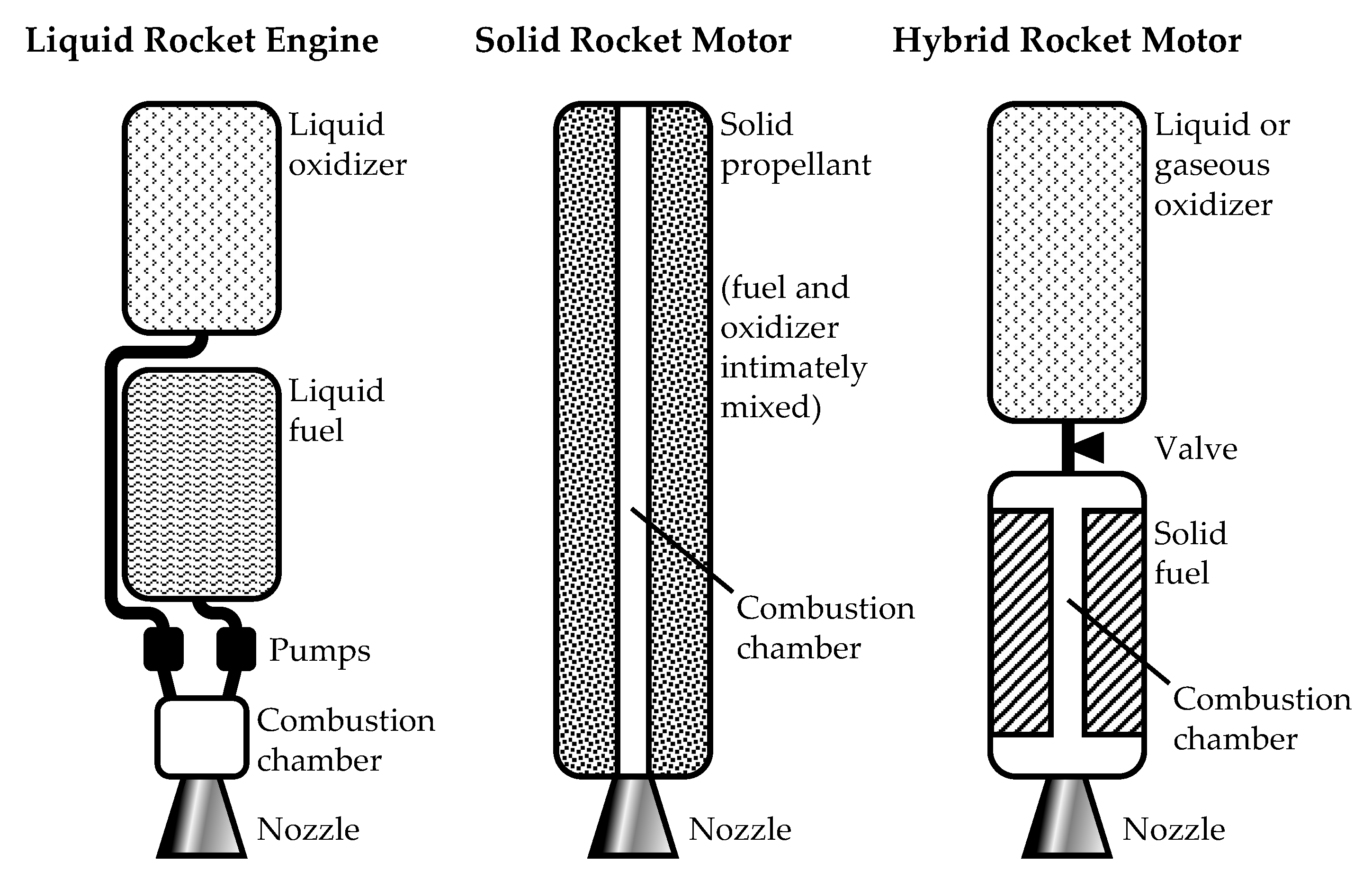
Article

Sensitivity Analysis of a Two-Phase CFD Simulation of a 1 kN Paraffin-Fueled Hybrid Rocket Motor

1
Royal Military Academy, Avenue de la Renaissance 30, 1000 Brussels, Belgium
2
École Polytechnique de Bruxelles, Aero-Thermo-Mechanics Department, Université Libre de Bruxelles, Avenue F.D. Roosevelt 50, 1050 Brussels, Belgium
*
Author to whom correspondence should be addressed.
Energies 2021, 14(20), 6794; https://doi.org/10.3390/en14206794
Submission received: 16 September 2021 / Revised: 12 October 2021 / Accepted: 14 October 2021 / Published: 18 October 2021
(This article belongs to the Special Issue Combustion and Propulsion Systems)

Abstract

:
At Université Libre de Bruxelles (ULB), research was performed on a 1 kN lab-scale Hybrid Rocket Motor (the ULB-HRM). It has a single-port solid paraffin fuel grain and uses liquid N 2 O as an oxidizer. The first Computational Fluid Dynamics (CFD) model of the motor was developed in 2020 and improved in 2021, using ANSYS Fluent software. It is a 2D axisymmetric, two-phase steady-state Reynolds-Averaged Navier–Stokes (RANS) model, which uses the average fuel and oxidizer mass flow rates as inputs. It includes oxidizer spray droplets and entrained fuel droplets, therefore adding many additional parameters compared to a single-phase model. It must be investigated how they affect the predicted operating conditions. In this article, a sensitivity analysis is performed to determine the model’s robustness. It is demonstrated that the CFD model performs well within the boundaries of its purpose, with average deviations between predicted and experimental values of about 1 % for the chamber pressure and 5 % for the thrust. From the sensitivity analysis, multiple observations and conclusions are made. An important observation is that oxidizer related parameters have the highest potential impact, introducing deviations of the predicted operating chamber pressure of up to 18%, while this is only about 6 % for fuel-related parameters. In general, the baseline CFD model of the ULB-HRM seems quite insensitive and it does not suffer from an excessive or abnormal sensitivity to any of the major parameters. Furthermore, the predicted operating conditions seem to respond in a logical and coherent way to changing input parameters. The model therefore seems sufficiently reliable to be used for future qualitative and quantitative predictions of the performance of the ULB-HRM.

1. Introduction

1.1. Hybrid Rocket Motors

A Hybrid Rocket Motor (HRM) is a type of chemical rocket motor. Chemical rocket motors are characterized by the reaction of a fuel with an oxidizer at some point in the motor. Depending on the way in which the fuel and oxidizer are stored, three types of chemical rocket motors exist: liquid, solid, and hybrid rocket motors (HRMs) [1]. In the latter case, the fuel and oxidizer are stored separately and in different phases. Figure 1 shows a schematic example of each of the three types of chemical propulsion systems. The illustrated HRM is the most common HRM configuration, which includes a solid fuel grain and a liquid or gaseous oxidizer.
Typical for an HRM is the formation of a non-premixed macroscopic diffusion flame in a large boundary layer, in which the fuel and oxidizer come together. This principle is shown in Figure 2, for the HRM configuration as shown in Figure 1, and it is based on the fundamental work on hybrid boundary layer combustion undertaken by [2].
An HRM combines some advantages of the solid and liquid motors, while eliminating some of their disadvantages. One of the main aspects are the safety and the complexity in terms of fabrication, handling, storage, and operation. During all of these stages, HRMs are far less hazardous or demanding than liquid or solid motors. From this, it follows that they are also less expensive and more accessible. Furthermore, HRMs can be throttled, shut down, and restarted [3].
Despite these promising properties, HRMs still lack technological maturity compared to solid and liquid systems, which are widely used for space launch, commercial and military applications. Although the specific impulse I s p of HRMs is competitive, hybrid rocket technology has been suffering throughout its history from low regression rates (resulting in low thrust), instabilities and other uncertainties when scaling up to full size motors for space launch applications. Given the successes of solid and liquid systems in the past, one could argue that the hybrid rocket technology has simply been overshadowed by them for a long time.
Nevertheless, there were some surges in the HRM research in the 1960s and 1980s. In the 1960s, the hybrid technology played an important role in target drones, for which a high thrust was not required. In the 1980s, the worldwide business in commercial satellites was growing. This caused a search for low-cost solutions to launch space vehicles, because of price competition. Also in the 1980s, in consequence of the Space Shuttle Challenger failure (1986), NASA (National Aeronautics and Space Administration) started a program in view of replacing the solid rocket boosters with HRMs. The program ended without success [3].
In the past two decades, there has again been a renewed interest in hybrid rocket technology. The safety, low cost, and therefore potential repeatability that come with HRMs, has become appealing again in the context of space tourism, satellite launch systems and in-space applications. A well-known accomplishment includes several successful flights of the Virgin Galactic SpaceShip, bringing tourists and researchers into space just above an altitude of 100 km, using an HRM propelled spaceship that is launched in-air from a carrier aircraft (air launch). Other recent hybrid rocket programs include the planned Turkish moon mission (2023) of DeltaV Space Technologies Inc., and the development of a commercial launch service by the Taiwanese company TiSpace. Apart from these larger programs, the HRM has always been popular amongst academic groups for use in their smaller sounding rockets or laboratory projects.
An important technological factor contributing to the renewed interest is the research on liquefying fuels such as paraffin wax. These fuels form a liquid layer at the fuel surface during operation, which can lead to the formation of roll waves from which fuel droplets can be entrained. This mechanism is illustrated in Figure 3 [4]. It results in regression rates that are 3 to 4 times higher than classical fuels, which can alleviate some of the aforementioned problems (low regression rate and thrust). Fundamental work on this is done by [4].

1.2. Computational Fluid Dynamics

In order to study the flow in HRMs, the fundamental partial differential equations (PDEs) of fluid dynamics have to be solved, such as the well-known Navier–Stokes equations, which describe the conservation of momentum. As an analytical solution of these equations is only feasible in very simplified cases, numerical methods are applied.
One of the first examples of this is presented in the book Weather Prediction by Numerical Process (1922) by [5]. By dividing the atmosphere, or in general, the fluid domain in discrete elements, the PDEs can be approximated by a system of algebraic equations, which can be solved iteratively. As computational power grew over the years, these equations could be solved by a computer, which is then referred to as Computational Fluid Dynamics (CFD) [6].
Although computational power has grown exponentially, there are still limitations. Practical flows such as in HRMs are highly turbulent, which requires an extremely high resolution domain discretization in order to capture all possible eddies. The smallest eddy is at the Kolmogorov scale, where viscosity dominates, and the turbulent kinetic energy is dissipated into heat. In the case of a paraffin-fueled HRM, which is the subject of this work, it is currently impossible to simulate the entire internal flowfield at such a level of detail (all possible length and time scales). Such a simulation is called direct numerical simulation (DNS). In addition, physical phenomena such as liquid droplet entrainment from the fuel surface, oxidizer spray, combustion and radiation, all add to the complexity of simulating an HRM. It is therefore necessary to adopt one of the simplified approaches presented below.
In CFD, there are two widely used alternatives to DNS that need far less computational power: Reynolds-Averaged Navier–Stokes (RANS) and Large-Eddy Simulation (LES). In RANS, the Navier–Stokes equations are averaged in time and space, and some model is chosen to include the effects of turbulence. The resulting solution is a smooth, averaged flowfield. If the simulated system is non-steady (changes with time), and if the associated timescales are much larger than the turbulent timescales, an unsteady RANS (URANS) simulation is possible, resulting in a series of average flowfields at different system times. LES is in essence a combination of DNS and RANS, in that the computed flowfield only includes the large eddies, while the smaller eddies are averaged. Note that RANS can be applied on a 2D or 3D mesh, while LES and DNS require a 3D mesh.

1.3. Research Scope

Since 2010, the Université Libre de Bruxelles (ULB) and the Royal Military Academy (RMA), both located in Brussels, are working together on a lab-scale HRM (referred to as the ULB-HRM in the remainder of the text). It has a target thrust of 1 kN and a theoretical burning time of about 10 s. The motor has a relatively short single-port solid paraffin fuel grain and uses liquid nitrous oxide ( N 2 O ) as an oxidizer, which is injected axially in a pre-combustion chamber. Figure 4 shows a typical image of the motor during operation, and Figure 5 shows a 3D cut of the motor and its main parts. Details about the internal geometry are presented in Section 2.1. For elaborate information on the ULB-HRM design process and the test bench development, the reader is referred to [7].
The past ULB-HRM research has been almost exclusively experimental. Examples include the HRM test bench development [7,8], the investigation of paraffin fuel properties [9,10], and the oxidizer injector development and their performance [11,12,13]. Some numerical work has been undertaken by [14], in which the influence of the fuel entrainment effect, mentioned at the end of Section 1.1, on the combustion properties of an HRM was investigated.
It is only recently, in 2020, that the ULB-HRM research was expanded with a first numerical model of the motor. It is a 2D axisymmetric single-phase (gaseous) steady-state RANS model, of which the results correspond well with the time-averaged experimental measurements (less than 10% offset) [15,16]. In 2021, this model was improved by adding a discrete liquid phase to account for both the nitrous oxide spray droplets and the entrained liquid fuel (paraffin) droplets. The results of this two-phase model show a very good agreement with the time-averaged experimental values: the average offset is 1% for the chamber pressure ( P c h ) and 5% for the thrust (F) [17]. The latter two-phase CFD model of the ULB-HRM forms the subject of the presented work.

1.4. Aim

The overall aim of the numerical work that started recently is to add a predictive capacity to the ULB-HRM academic research and, ultimately, improve the ULB-HRM. This is achieved by developing numerical models of the ULB-HRM with increasing complexity. At this stage, the latest model uses the time-averaged oxidizer and fuel mass flow rates as inputs. These two parameters are known from the experiments. By using these experimental values as inputs, the predicted motor operating conditions can be compared with experimental measurements. As mentioned in Section 1.3, the latest two-phase model performs well at this level. It therefore allows to predict, to some extent, the motor’s performance for a given oxidizer and fuel mass flow rate. Note that, in reality, the fuel mass flow rate depends on the oxidizer mass flow rate. Therefore, ideally, future numerical models of the ULB-HRM should also solve for the fuel regression rate (from which the fuel mass flow rate is obtained), therefore only using the oxidizer mass flow rate as input. In addition, the fuel mass flow rate can also be estimated by using an empirical relation such as r ˙ = a G o x n [2], which relates the fuel regression rate r ˙ to the oxidizer mass flux G o x in the fuel port, by using only two empirical constants, a and n. This is actually a simplified equation, as a series of parameters are lumped into a single empirical constant a.
The specific aim of the presented work here is to provide some details about the latest two-phase CFD model, and to investigate its sensitivity to a series of input parameters. This provides insights into how the flowfield and the motor’s operating conditions are affected by these parameters, and it allows to identify the level of uncertainty they introduce in the numerical results. From this, conclusions about the overall robustness of the model can be drawn. This part of the investigation is essential before applying the model to perform qualitative or quantitative predictions about the behavior of the ULB-HRM, such as with respect to changes in geometry.

1.5. Outline

In Section 1, all the necessary elements have been provided for the reader to place this work in its context. In Section 2, the latest two-phase model with its baseline input parameter values is presented. Next, in Section 3, a sensitivity analysis with respect to a series of input parameters is performed by deviating from their baseline values. In the final section, Section 4, the presented work and the conclusions are summarized.

2. Baseline CFD Model

2.1. Computational Domain

The computational domain is a 2D axisymmetric domain, which includes the internal geometry of the motor and an exhaust plume area. This allows to investigate the exhaust plume itself, and it avoids having to set a boundary condition directly at the nozzle exit. By using a 2D mesh instead of a 3D mesh, the computational time is reduced significantly and therefore many simulations can be performed in a relatively short amount of time. This is an important feature, as many parameters have to be investigated to perform a good sensitivity analysis (see Section 3). Many of the conclusions that follow from this analysis may also apply for future, more complex models such as 3D LES models, for which the computational time is increased dramatically. For those models, the available computational power will most likely limit the extent to which a sensitivity analysis can be done, so that assumptions based on conclusions from a 2D analysis must be made. Figure 6 shows the computational domain, which is represented by the white area, its dimensions, and, for clarity, the surrounding parts of the motor. The size of the exhaust plume area is based on observations of the exhaust plume during experiments with the ULB-HRM. During these experiments, the intermediate port radius is 35 mm, for which the reason is explained later in Section 2.3.1.

2.2. Mesh

The current mesh is a structured-like mesh, and it consists of 120,602 cells, which are almost all quadrilateral (Figure 7). The mesh was created using the ANSYS Meshing tool. The mesh convergence study for the single-phase model resulted in a characteristic cell size Δ x c h a r of 1 mm in the combustion chamber [15]. As the current model is a two-phase model, the mesh convergence must be reviewed. Therefore, the baseline simulation of experiment “SH1-01” (a list is provided in Section 2.6) is performed on three different meshes. A diagram is provided in Figure 8, in which the resulting numerical chamber pressure P c h and mass averaged nozzle exit velocity v ¯ e x i t are shown as a function of Δ x c h a r . From this, it is concluded that the resulting operating conditions still remain quasi unchanged below Δ x c h a r = 1 mm, as it was the case for the single-phase model. Therefore, it seems acceptable to continue with the same 1 mm mesh that was used for the single-phase model. The mesh has a near-wall refinement to account for the effects of the viscous sublayer near the wall. More information on this is presented in [15].

2.3. Flow Modeling

In contrast to the first CFD model of the ULB-HRM, the latest model is a two-phase model. A continuous gas phase is solved in a Eulerian framework, and a discrete liquid phase is solved in a Lagrangian framework. The discrete liquid phase is introduced to mimic the effects of the injected oxidizer spray and entrained fuel droplets. Both phases interact through Eulerian–Lagrangian coupling, but the discrete liquid droplets do not break up or interact with each other. Details on how the gaseous and liquid oxidizer and fuel enter the domain are provided in Section 2.5.

2.3.1. Continuous Gas Phase

The steady-state RANS model is used to simulate the continuous gas phase in the ULB-HRM. The resulting flowfield, therefore, represents the average operating conditions of the motor, when the fuel grain thickness is about half the initial web thickness b (definition provided in [1]). This is why the port radius in the numerical domain is set to 35 mm (see Section 2.1). At this stage of the numerical research, this approach is acceptable for the development of the initial CFD models of the motor. Moreover, some of the experimental measurements to which the numerical results are compared, are only available as space-time averaged values.
The Reynolds averaging process of the momentum conservation equations leads to the well-known RANS equations, in which a Reynolds stress term appears, which can be modeled by applying a turbulence model. In the presented CFD model, the k- ϵ eddy viscosity model [18] is applied. This choice is motivated by the preliminary lack of success with other turbulence models such as the k- ω model [19] or the k- ω SST model [20], for which the results are unrealistic or not attained at all due to convergence issues.
Next, the resulting governing equations are presented in which source terms appear to establish the coupling between the continuous gas phase and the discrete liquid phase. The first equation presented below is the continuity equation or mass conservation equation.
ρ t + · ( ρ v ) = S m
The source term S m represents the mass that is added to the continuous phase from the evaporation of the discrete liquid phase. Similarly, due to the exchange in momentum caused by drag forces between the gas phase and the liquid droplets, a force source S F appears on the right hand side in the RANS equations (conservation of momentum). Note that Equation (2) can be written as multiple equations (one for each component of v ), hence the plural RANS equations is most often used.
t ( ρ v ) + · ( ρ v v ) = P + · ( μ + μ t ) ( v + v T 2 3 · v I ) + · ( ρ k 2 3 I ) + S F
In the total energy equation, shown below in terms of enthalpy H, two source terms appear. The heat of combustion is responsible for the first source S H , c . The heat exchange between the continuous and the discrete phase is represented by the second source term S H , d .
t ( ρ H ) + t ( ρ K ) + · ( ρ v H ) + · ( ρ v K ) P t = · κ + κ t c p H + S H , c + S H , d
Because of the chosen combustion model, presented later in Section 2.4, several species must be tracked separately. Therefore, the model also includes N-1 transport equations for the N species that are present in the calculation. Furthermore, given the k- ϵ turbulence model, two additional transport equations for k and ϵ are solved as well.
A detailed list of all the equations involved in describing the continuous gas phase, starting from the general convection-diffusion equation for any extensive property ϕ , is presented in [15] and is therefore not repeated here. Details on how the various source terms are calculated can be found in [21].

2.3.2. Discrete Liquid Phase

For the discrete phase, the trajectory of a droplet is predicted by integrating the force balance on it, which is written in a Lagrangian reference frame. In this case, the only force acting on the droplets is a drag force. This results in the following equation, in which the indices c and p refer to continuous phase and particle (droplet), respectively.
d v d t = 3 C D ρ c 4 d p ρ p | v c v p | ( v c v p )
For an evaporating droplet, the temperature is calculated using the equation below, in which h is the convective heat transfer coefficient and h p , v a p is the droplet vaporization enthalpy. It does not include the term for radiation, as the latter is ignored in the developed model.
m p c p d T p d t = h A p ( T c T p ) d m p d t h p , v a p
For specific details such as the calculation of the drag coefficient C D and the droplet vaporization rate d m p d t , the reader is referred to [21].

2.4. Combustion Model

Typical for an HRM, as indicated in Section 1.1, is the macroscopic turbulent diffusion flame that is formed where the oxidizer and fuel meet in flame sustaining quantities. Heat transfer from the flame to the fuel surface causes the fuel to evaporate towards the flame zone, which sustains the combustion process. Fundamental work on the diffusion flame in both classical and paraffin fueled HRMs is presented in [2,4], respectively.
In this work, a high Damköhler number is assumed, meaning that the chemical reaction rate is much higher than the convective mass transport rate. For the flow in an HRM, it implies that the combustion rate is controlled by the turbulent mixing. To model this turbulence–chemistry interaction (TCI), the Eddy Dissipation Model (EDM) [22] is chosen. The model requires a transport equation for each species, but it avoids complex chemical kinetics. The EDM is one of the popular choices and it has proven to provide good results. Examples include [23,24,25]. Another well-known model is the mixture fraction model [26]. Preliminary results (single-phase) have been obtained with this model [16], confirming that it is a viable alternative to the EDM.
In the EDM, the reaction rate is calculated based on the turbulence field values k and ϵ . Therefore, only one reaction rate is calculated, and a single global chemical reaction must be provided. In order to establish this chemical equation, the reactants must first be determined. For the oxidizer this is N 2 O . For the fuel, the main products of the pyrolysis of paraffin are consideroxider ed. The pyrolysis of paraffin with chemical formula C n H 2 n + 2 yields the following products.
C n H 2 n + 2 = H 2 + n 2 C 2 H 4
In order to test the impact of the presence of H 2 in the paraffin pyrolysis products, a preliminary numerical investigation was performed with and without the H 2 in the reactants. It was found that the impact on the resulting numerical flowfield is negligible and therefore only ethylene ( C 2 H 4 ) is considered as fuel reactant. For an ideal combustion of C 2 H 4 with N 2 O , the reaction is as follows.
C 2 H 4 + 6 N 2 O = 2 C O 2 + 4 H 2 O + 6 N 2
This reaction was considered in the first single-phase CFD model presented in [15]. In reality, however, a series of reaction products exist in chemical equilibrium. Therefore, instead of driving the reaction towards the products as shown in Equation (7), the reaction is now driven towards some equilibrium composition. As it will become clear in Section 2.6, 19 experiments are simulated and therefore a composition of the reaction products must be estimated for each one of them. This is done with ICT-code (thermodynamic code from Fraunhofer Institute for Chemical Technology) [27], based on the experimental chamber pressure P c h , exp for each case. The obtained reaction for test SH1-01 is shown below. The considered reaction products represent just over 97 m% of all products generated by ICT-code. Note that, as expected, the same results were obtained with NASA’s CEA (Chemical Equilibrium and Applications) [28].
C 2 H 4 + 6 N 2 O = 5.867 N 2 + 1.542 H 2 O + 1.107 C O + 0.893 C O 2 + 0.43 O H + 0.4345 O 2 + 0.266 N O + 0.243 H 2
Based on the reaction coefficients in this equation, the EDM calculates R i , which is the rate of production of species i, as the smallest of the two equations below [22]. R i appears as a source term in the ith species transport equation.
R i = ( ν i ν i ) M i A ρ ϵ k min R Y R ν i M R
R i = ( ν i ν i ) M i A B ρ ϵ k P Y P j ν j M j
Note that the droplets that are present in the flow do not react themselves, but they evaporate. The evaporated gas then reacts according to the model described above. The liquid N 2 O droplets evaporate to gaseous N 2 O , and the liquid paraffin droplets evaporate to gaseous ethylene. In short, all reactions occur in the gas phase.

2.5. Boundary Conditions

In Section 2.1 through Section 2.4, all physicochemical models and flow equations are determined. The numerical solution or resulting flowfield now ultimately depends on the boundary conditions. For the baseline CFD model that is presented in Section 2, many aspects of the boundary conditions are fixed at some motivated value. The only parameters that are not fixed are the total oxidizer inlet mass flow rate m ˙ o x (and from it, the inlet velocity v o x ) and the total fuel inlet mass flow rate m ˙ f u e l , as these values depend on the experiment that is being simulated. As mentioned in Section 1.4, the experimental time-averaged oxidizer and fuel mass flow rates serve as input to the numerical model at this stage of its development. In order to easily locate the different boundary conditions that are discussed in the following sections, an overview is provided in Figure 9.

2.5.1. Oxidizer Inlet

In Section 2.6, 19 experiments will be simulated with the baseline CFD model. The purpose is to compare the numerical results with the experimental measurements. During all 19 experiments, a showerhead (SH) injector was used to inject the liquid N 2 O . However, not all experiments were performed with the exact same SH injector. In fact, four types of SH injectors were used. A summary is shown in Table 1.
In order to model the oxidizer injection in a 2D axisymmetric domain, a simplification must be made, as it is not possible to model the individual orifices. Therefore, in the simulations, the oxidizer is injected in the normal direction from a Ø 70 mm circular area as a mixture of gas and liquid droplets (see Figure 9).
The presence of two oxidizer phases (rather than only liquid) results from the oxidizer flow development within the injector orifices. Some mass fraction, called the vapor quality x, therefore leaves the injector as a gas. Since only the total average oxidizer mass flow rate is known from the experimental results, some estimation of x must be made. In [30], different injector flow modeling options are explored and summarized. A possible way to determine x is to consider an isentropic depressurization throughout the orifices. During this process, it is assumed that the liquid and vapor have equal velocities and are in thermodynamic equilibrium. This model is referred to as the Homogeneous Equilibrium Model (HEM). In this case, we can write for x:
x = s 1 L s 2 L s 2 V s 2 L
where 1 and 2 refer to upstream and downstream conditions of the orifice, respectively, and L and V refer to the saturated liquid and vapor, respectively. As the experimental pressures before and after the injector are known, the entropy values can be taken from a thermophysical properties database such as the one provided by the National Institute for Standards and Technology (NIST) [31]. The average values that are found for x using Equation (11) are between 14% and 22%, and therefore a value of 20% is chosen for all 19 baseline simulations. In [24], a very similar HRM test bench setup with nitrous oxide is investigated and similar values for x have been found.
Next, the size of the liquid N 2 O droplets must be estimated as well. Usually, some empirical size distribution function is used. However, no distribution is universally better than any other, and the extent to which any particular function matches any given set of data depends largely on the mechanism of disintegration involved [32]. Therefore, at this stage of the two-phase model development, all droplets are set to have the same diameter (uniform size distribution). This allows for a clear initial analysis of the droplet size influence. Future work can include exploring a non-uniform size distribution such as the popular Rosin-Rammler distribution [33].
To determine the uniform diameter, some representative mean value should be chosen. There are several definitions for a mean diameter. The most widely used mean diameter is the Sauter Mean Diameter (SMD) or D 32 . Definitions of different mean diameters are presented in [32]. The SMD is the diameter of the drop whose ratio of volume to surface area is the same as that of the entire spray. Empirical expressions for the SMD in the case of plain orifices, such as those of the current SH injectors, have been established by several researchers [32]. Unfortunately, the resulting SMDs can be unreliable, as the conditions in the ULB-HRM can deviate significantly from those for which the empirical expressions of the SMD are valid. On top of this, it is also difficult to insert the appropriate values for some of the gas and liquid properties in those expressions. Both in [29,34], the SMD of N 2 O spray was estimated for similar injectors, and it was found to be around 0.3 and 1000 µm, respectively. This shows how easily results can deviate. An example calculation for test SH1-01, based on [35], is shown below and yields 274 µm.
S M D = 500 d or 1.2 ν ox 0.2 v ox = 500 · 0 . 0014 1.2 · 8.036 · 10 8 0.2 26.18 = 0.000274 m = 274 μ m
in which ν ox is the liquid oxidizer kinematic viscosity, and d or is the orifice diameter. The oxidizer inlet velocity v ox (only required for the liquid droplets) is calculated as
v ox = m ˙ ox , exp ρ ox A or
From all the above, it can only be concluded that the droplet SMD is expected to lie between 1 and 1000 µm. Therefore, an intermediate reference value of 100 µm is chosen for the baseline simulations, based on the order of magnitude found from Equation (12), as well as from another expression provided by [36], which yields 333 µm.
The last inputs that are needed, are the thermophysical properties of N 2 O . They are taken from [31,37].
To end this section, a summary of the oxidizer boundary conditions is provided in Table 2.

2.5.2. Fuel Inlet

The location of the fuel grain has already been shown in Figure 6. In the numerical baseline model, fuel enters the domain both as a gas ( C 2 H 4 , see Section 2.4) and as liquid droplets (paraffin) with an initial velocity normal to the grain surface (see Figure 9). The droplets enter the domain from the grain surface, and the gaseous fuel enters the domain as sources in the cells adjacent to the grain surface. The grain surface itself is a wall boundary. No fuel enters the domain from the sides of the fuel grain.
Similar to the oxidizer inlet (Section 2.5.1), 19 time-averaged experimental fuel mass flow rates ( m ˙ fuel , exp ) serve as input for the 19 simulations that are presented later in Section 2.6. For the ULB-HRM, it is however unclear which fraction of m ˙ fuel , exp is entrained as a result of the liquid film formation mentioned in Section 1.1.
An estimation is made based on the work presented in [38], in which it is explained that the entrainment rates for the liquefying fuel pentane are close to those of paraffin wax. Also in [38], a liquid layer theory is developed, and the diagram shown in Figure 10 is established based on that theory. It includes entrainment predictions for pentane as a function of the total port mass flux.
For the average fuel port radius of 35 mm that is chosen for the baseline simulations presented in the current work, the total port mass flux ranges from 100 to 180 k g m 2 s , depending on the experiment and on the axial position in the fuel port. For these fluxes, the estimated mass fraction of entrained fuel ranges from 46 to 59%, respectively. Therefore, the entrained fuel mass fraction is set to 50% for all 19 baseline simulations.
Next, some choice has to be made for the liquid fuel droplet diameter. For the same reasons as explained in the previous section on the oxidizer inlet, a uniform size distribution is chosen for the baseline numerical model. In order to determine some representative diameter, the empirical relation of [39] shown below is applied, as suggested by [40] to be the most representative for fuel droplet size prediction in an HRM.
D v m = 0.028 σ ρ g j g 2 Re f 1 6 Re g 2 3 ρ g ρ f 1 3 μ g μ f 2 3
Here, D v m is called the volume median diameter. By definition, the total volume of all droplets with a diameter larger than D v m , is 50% of the total volume of all droplets. The subscripts f and g refer to the properties of the fuel liquid film and of the gas flowing over the liquid film. The gas flow velocity over the liquid film is represented by j g . The Reynolds numbers are based upon the hydraulic diameter d h , which is set to be the port diameter.
Re f = ρ f j f d h μ f
Re g = ρ g j g d h μ g
Here, j f is the liquid film flow velocity. By replacing Re f and Re g in Equation (14) by Equations (15) and (16), Equation (14) becomes
D v m = 0.028 σ d h 1 2 ρ g 2 3 j g 4 3 ρ f 1 6 j f 1 6 μ f 1 2
It is of course not easy to determine the correct thermophysical properties and velocities that could apply for the ULB-HRM. They depend on many aspects such as the temperature, the distance from the liquid film and the axial position. By using Equation (17), it is assumed that the obtained volume median diameter only represents some order of magnitude. Based on data from [14,31], together with observations of the numerical flowfield, Table 3 is established. It shows the expected fuel droplet volume median diameter D v m for a set of baseline values for the parameters that are present in Equation (17). Next, in Table 4, the influence of each of these parameters on D v m is shown. Each line represents the variation of D v m when the value of a certain parameter is changed within some range of uncertainty, while keeping the others parameters at their baseline value. With an exponent of 4 3 , it is clear that the gas flow velocity j g has the most impact.
Based on this short analysis, the representative value for the uniform size of the fuel droplets is estimated to be of the order of 100 µm.
The initial velocity of the fuel droplets is based on the velocity flowfield, which was obtained with the first single phase numerical model [15]. In this model, fuel enters the domain as gaseous C 2 H 4 at a mass flow rate of m ˙ fuel , exp . The resulting average radial velocity near the grain surface is used for the initial fuel droplet velocity in the current two-phase model, and it is equal to 0.28 m/s. In the work of [9], a value of the same order of magnitude is obtained.
Although the conditions in the ULB-HRM are for the most part beyond the paraffin wax critical conditions, some initial temperature must be set for the gaseous and liquid fuel that enters the domain. A common approach is to set the temperature of the droplets as the average of the paraffin melting and boiling temperature, which yields 515 K. The grain wall is also fixed at this temperature. For the gaseous fuel ( C 2 H 4 ), the inlet temperature is set to the boiling temperature, which is 700 K.
Table 5 summarizes the fuel boundary conditions. Thermophysical properties for paraffin wax and ethylene are taken from [31], as well as from previous experimental work on the ULB-HRM [7,14].

2.5.3. Walls

Figure 9 shows the locations of the wall type boundaries. They are all no-slip walls that reflect any droplets colliding with them. A detailed study of these collisions and their simulation falls outside the scope of this work. All walls are adiabatic, except for the grain wall (see Section 2.5.2).

2.5.4. Ambient Inlet and Outlet

As shown in Figure 9, the ambient area consists of a 1 atm pressure outlet and a lateral 1 atm pressure inlet (air at 280 K). The latter allows for the exhaust plume to draw in air from the sides.

2.6. Baseline Model Results

The baseline CFD model is now used to simulate 19 experiments, which are listed in Table 6. Showerhead 1 leads to 10 “low pressure” cases (order 17 bar), and showerheads 2, 3 and 4 lead to 9 “high pressure” cases (order 24 bar). The four types of SH injectors are summarized in Table 1. The purpose of Table 6 is to compare the numerical results with the experimental results, and draw conclusions about the performance of the model. Typical computational times range from a few hours to one day, depending on the values of the input parameters, such as droplet sizes and liquid fractions. Note that the experimental results are not used to calibrate the CFD model in any way. Before comparing the results, some visualizations of the flowfield are provided first.
In Figure 11, a visualization of the flowfield in terms of the static temperature for cases SH1-04 and SH4-04 is shown. It shows the cases for which the highest and lowest numerical chamber pressures are obtained, respectively.
Next, in Figure 12, the streamlines are shown for case SH4-04. Two recirculation zones are easily identified. The recirculation zone in the pre-combustion chamber extends slightly into the fuel port, causing fuel (both droplets and gas) to enter the pre-combustion chamber, where it can react with the oxidizer. This phenomenon was also observed during the experiments, confirmed by the paraffin wax that was found on the oxidizer injector plate after the test run [13].
In order to compare the numerical results with the experimental measurements, two diagrams are provided in Figure 13.
On the left diagram, the numerical and experimental chamber pressures P c h are plotted on the ordinate and abscissa, respectively. As all cases are very close to the central identity line, it is clear that the model predicts P c h accurately.
On the right diagram, the same plot is presented for the thrust F. The same conclusion as for P c h holds, but there is a slight overestimation of F for the high pressure cases (groups “SH2”, “SH3”, and “SH4”). A possible reason for this is an overestimation of the chemical reactions in the nozzle, leading to an overestimated nozzle exit velocity (from which F is calculated). However, it might also be due to certain phenomena causing performance losses during the experiments, so that the expected thrust is not reached for higher chamber pressures.
Section 2 is concluded with Table 7, in which the average deviations between the numerical and experimental values are summarized. With average deviations of + 1 % and + 5 % for P c h and F, respectively, it can be concluded that the model performs well. It must, however, be noted that the model does not include all physical phenomena that occur in the ULB-HRM. This implies that there might be hidden deviations that compensate for each other. Nevertheless, the model demonstrates the potential to perform predictions about the operating characteristics and performance of the ULB-HRM, when installed with an SH injector.

3. Sensitivity Analysis

In this section, a sensitivity analysis is performed. As indicated in Section 1.4, this is performed by varying a series of model input parameters and monitoring the effect on the resulting operating conditions of the motor. From this, conclusions can be drawn about
  • The level of uncertainty introduced in the numerical results;
  • The overall robustness of the numerical model;
  • How the flowfield is affected qualitatively;
  • How the ULB-HRM would react to changing boundary conditions.
The selected input parameters of the baseline CFD model are now reviewed in the same order as they were presented in Section 2. Note that, unless mentioned otherwise, only one parameter at a time is investigated, while keeping the other parameters at their baseline value. The range for each parameter is chosen such that it reflects the limits of what can be expected in reality.

3.1. Combustion Model

3.1.1. Chemical Reaction Equation

The stoichiometric coefficients of the products in Equation (8), which was presented in Section 2.4, are valid for some specific chamber pressure P c h , which in turn depends on these coefficients. Therefore, their determination should ideally be an iterative process. As this would be very time consuming, the chemical reaction equations for the 19 simulations have been determined via ICT, based on the experimental chamber pressure P c h , exp . They are summarized in Table 8, in which the stoichiometric coefficients of Equation (8) are found at the first line.
From Table 8, it is immediately clear that the coefficients vary very little within the range of relevant chamber pressures. To quantify the influence of the coefficients on the resulting numerical chamber pressure P c h , num , two extra simulations are performed. The case with the lowest P c h , exp , case SH1-02, is simulated as before, but by applying the coefficients of SH3-03, the case with the highest P c h , exp . Likewise, the case with the highest P c h , exp , case SH3-03, is simulated as before, but by applying the coefficients of SH1-02. The effect on P c h , num by applying these incorrect coefficients is very limited, as shown in Table 9. It can be concluded that a single set of product coefficients would be sufficient to simulate all 19 cases. The maximum error would then be about 0.2%.

3.1.2. Chemistry in Nozzle

In the baseline CFD model, the EDM is active throughout the entire numerical domain. While hot gasses expand in the nozzle, their chemical composition changes as the chemical reactions continue. This is called shifting equilibrium, and it often leads to slightly overestimated performance values. Another approach is called frozen equilibrium, in which case the chemical composition remains constant throughout the nozzle expansion process. This approach tends to underestimate the system’s performance [1].
In order to determine the effect of setting the nozzle to a frozen equilibrium instead of a shifting equilibrium, the simulations of the experiments SH1-04 and SH4-04 are run again with deactivated reactions in the nozzle and ambient area. Figure 14 shows the temperature flowfield of the simulation of experiment SH4-04, for both shifting and frozen equilibrium in the nozzle. Next, in Figure 15, the impact on P c h , num and F num is visualized. For the two cases, P c h , num is reduced by maximum 5%, and F num is reduced by a maximum of 15%. Therefore, as it could be expected, the largest impact is observed on the thrust.
As mentioned before in Section 2.6, the baseline model slightly overestimates the thrust for the high pressure cases. It was speculated that, for these cases, the chemical reaction progress might be overestimated in the nozzle. This can be related to the combustion model, which predicts the reaction progress based on the turbulence. From Figure 14, it is clear that there is a high level of turbulent mixing immediately downstream the throat. If the k- ϵ model overpredicts the turbulence in that region, the reaction progress will be overestimated as well. However, from the analysis in the current section, it is clear that a frozen equilibrium in the nozzle (no reactions) has an almost equally important impact on the thrust of SH1-04 as on that of SH4-04. It can therefore be concluded that the overestimated thrust is not (only) caused by an overestimation of the reactions.
Furthermore, it can be concluded that the baseline CFD model is quite sensitive to whether the flow in the nozzle is frozen or shifting. However, although this is an interesting observation, such an important and non-quantifiable parameter could be as important as the selection of the combustion model itself. Therefore, one could argue about whether this element falls within the boundaries of a sensitivity analysis.

3.2. Oxidizer Inlet

3.2.1. Vapor Quality

In Section 2.5.1, the vapor quality x for the N 2 O inlet was set to 20% for the baseline CFD model. This value is now investigated by varying it from 0 to 100%. The impact on P c h , num and F num is visualized in Figure 16. For SH2-01, both P c h , num and F num show a maximum near the baseline value of 20%. For SH1-01, this is for x [ 0.20 , 0.40 ] . From this, it is concluded that x affects the motor’s operating conditions not in a linear but rather parabolic way, due to a combination of different effects on the flowfield which are visualized and discussed later in this section.
Table 10 and Table 11 summarize some key values from the diagrams in Figure 16. Based on the study of cases SH1-01 and SH2-02, it is concluded from Table 10 and Table 11 that the uncertainty of the vapor quality x can introduce a maximum absolute deviation of P c h , num and F num from their baseline values of the order of 18% and 8%, respectively. This demonstrates how the CFD model would not be accurate if the liquid phase of the oxidizer would be ignored by assuming an all gaseous oxidizer inlet. Moreover, it is reasonable to assume that x will never reach values of 100% in the ULB-HRM. Within the range of 0 to 50%, the deviations mentioned above are only of the order of 5% and 2%, which adds to the robustness of the developed model. Another observation is that the baseline value of x (20%) results in the highest (or almost highest) values for the numerical chamber pressure and thrust, from which it can be concluded that any other value for x leads to a lower prediction of the motor’s performance in terms of P c h and F. For design purposes, an SH injector that delivers a vapor quality of about 20 to 30% therefore seems optimal.
Next, the effect of x on the flowfield is investigated. Figure 17 shows the static temperature contours and droplet trajectories for case SH1-01, for x { 0 , 0.2 , 0.7 , 1 } . Only the upper half of the domain is shown for compactness. A remarkable impact on the average temperature in the pre-combustion chamber ( T pre ) is observed. As x increases, fewer oxidizer droplets are injected into the fuel port and therefore the recirculation zone mentioned in Section 2.6 extends less into the upstream end of the fuel port, as illustrated in [17]. As a consequence, less fuel is reacting with the oxidizer upstream in the pre-combustion chamber, explaining a decreasing temperature with increasing x. In the post-combustion chamber, however, T post seems to reach a maximum for x = 20 % , just as it was the case for P c h , num and F num . For this value, the amount of fuel recirculation in the pre-combustion chamber, together with the oxidizer droplets trajectory and lifetime throughout the combustion and post-combustion chamber, seem optimal to reach the highest chamber pressure. Note that for higher values of x, unburnt fuel droplets start exiting the motor.

3.2.2. Spray Droplets Size

The oxidizer spray droplets diameter ( d ox ) was set to a uniform distribution of 100 µm for the baseline CFD model, as explained and motivated in Section 2.5.1. In the current section, the impact of this diameter is investigated while the uniform size distribution is maintained. Figure 18 shows the influence of d ox on P c h , num for cases SH1-01 and SH2-01. The plot of F num is not included as it follows the same profile as P c h , num . This was also the case for the study of the vapor quality x in Section 3.2.1.
From Figure 18, it is clear that, within the investigated range of d ox , P c h , num decreases non-linearly with decreasing d ox . As the droplet size decreases, the derivative of P c h , num ( d ox ) increases substantially, indicating a higher sensitivity of the motor’s performance to size variations within the range of smaller droplets.
Table 12 summarizes some key values of the plot from Figure 18. It is concluded that the uncertainty of d ox can introduce a maximum absolute deviation of P c h , num of about 16% from its baseline value, when d ox varies between 20 and 500 µm. Note that Table 12 also includes some extrapolated values, for which the reason is explained next.
From a physical point of view it is expected that when d ox approaches 0 µm, the numerical results should approach those of the case where the oxidizer is injected completely as a gas. From Table 10, it can be seen that for case SH1-01, P c h , num equals 14.80 bar when x = 100 % (all injected oxidizer is gaseous). This is indeed very close to the pressure obtained by extrapolating the curve in Figure 18 to a theoretical d ox of 0 µm with a fourth-order polynomial fit, which then yields 14.85 bar. This adds to the robustness and the consistency of the CFD model.
Figure 19 visualizes how the flowfield is affected by the oxidizer droplets diameter d ox in terms of the static temperature. It stands out immediately that the temperature in the pre-combustion chamber increases significantly with decreasing d ox , and reaches a maximum for d ox 40 to 60 µm, after which it decreases again for smaller values of d ox . This behavior is possibly related to the oxidizer droplet pathlines along which they evaporate and is currently under further investigation.

3.3. Fuel Inlet

3.3.1. Entrained Fuel Fraction

Based on the literature, it was estimated in Section 2.5.2 that 50% of the total experimental fuel mass flow rate ( m ˙ fuel , exp ) consists of entrained fuel droplets. This entrained fuel fraction, x ent , is a parameter comparable to 1 x (with x the vapor fraction of oxidizer, see Section 2.5.1 and Section 3.2.1). As it is very difficult to confirm this baseline value of 50% experimentally, it must be investigated how x ent , as a user input of the CFD model, affects the numerical results. In this section, x ent is varied from 0 to 100%, while keeping the total numerical fuel mass flow rate constant and equal to the corresponding average experimental value m ˙ fuel , exp . The focus is again on P c h , num , as this is a measurable key operating value.
Figure 20 demonstrates how the numerical chamber pressure P c h , num is affected by x ent in the simulations of eight experiments (4 low pressure cases and 4 high pressure cases, see Section 2.6). It is clear that the curves of P c h , num ( x ent ) follow the same quasi-linear (especially for x ent < 67 % ) profile for all eight cases. As x ent increases, P c h , num decreases. This might seem strange at first, as the entrainment of the paraffin fuel droplets is known to improve the fuel regression rate and therefore the motor’s performance. However, in that case, the total fuel mass flow rate is increased by the entrainment effect. In the current sensitivity analysis, however, the total fuel mass flow rate is kept constant as clearly indicated at the abscissa in Figure 20. Whenever x ent increases, the mass flow rate of entrained droplets increases at the cost of an equal decrease in the mass flow rate of gaseous fuel entering the domain. Increasing x ent simply implies that more droplets first have to evaporate before they can take part in the reaction.
For completeness, it is demonstrated in Figure 21 how the chamber pressure would be affected if the gaseous fuel flow rate is kept constant while some entrained fuel is added, thus increasing the total fuel mass flow rate. This is done by starting from the simulation of SH1-01 with x ent = 0 . It is clear from the diagram that, for some given oxidizer mass flow rate, the motor’s performance does indeed benefit from the entrainment effect. Note that Figure 21 shows the chamber pressures that would be reached theoretically, if one would be able to achieve a certain fuel mass flow rate and entrainment with the given oxidizer mass flow rate. In reality, there is of course a limitation to the fuel regression rate that can be achieved for some given oxidizer mass flow rate.
Table 13 summarizes some key values from the plot in Figure 20. It is concluded that the uncertainty of x ent can introduce a maximum absolute deviation of P c h , num of about 4% from its baseline value, when x ent varies between 0 and 100%. As explained in Section 2.5.2, it is estimated that the entrained fuel fraction ranges from 46 to 59%, based on the operating conditions of the 19 experiments. With this in mind it would be safe to state that the actual entrained fuel mass fraction lies somewhere between 33% and 67%. Within this range, the CFD model is quite insensitive, with a maximum deviation from the baseline pressure of only 0.8%.
To conclude this section, the temperature contours corresponding to the five points of the curve for SH1-01 in Figure 20 are shown in Figure 22. From the colormap, it is observed that, as x ent increases, the average temperature in both the pre- and post-combustion chamber decreases together with P c h , num . Furthermore, the width of the macroscopic boundary layer decreases with increasing x ent . For x ent = 100 % , it is clear that the diffusion flame is less wide and burns hotter in the post-combustion chamber than for lower values of x ent . The reason for this is that, as explained earlier in this section, droplets first need to evaporate before taking part in the reaction. When x ent = 100 % , gaseous fuel enters the domain along the pathlines of the fuel droplets, whereas for x ent = 0 % , the fuel (all gaseous) enters the domain along the grain surface.

3.3.2. Entrained Droplets Size

In Section 2.5.2, the entrained fuel droplets size was set to a uniform 100 µm for the baseline CFD model. In the current section, the impact of the fuel droplets diameter d ent is investigated for d ent ranging from 10 to 5000 µm. As before, the focus lies on the numerical chamber pressure P c h , num , as other performance parameters such as the thrust are impacted in the same (qualitative) way as P c h , num .
Figure 23 demonstrates how P c h , num relates to d ent for SH1-01 and SH2-01. The diagram also includes a plot of the fraction of the total mass flow rate that exits the motor as liquid droplets, denoted by x exit , and thus defined as
x exit = m ˙ liq . , exit m ˙ total
For both the low (SH1-01) and high (SH2-01) pressure case, it is concluded from Figure 23 that d ent has little impact on P c h , num , as long as no unburnt fuel droplets exit the motor. According to the CFD model, this starts to occur when d ent exceeds 100 µm. For d ent > 100 µm, x exit is non-zero and increases with increasing d ent , which means that an increasing fraction of the total mass flow rate at the nozzle exit is liquid. This fraction consists of fuel droplets only, as it is known that no unreacted oxidizer droplets exit the nozzle when all oxidizer parameters are set to their baseline values (see Figure 17 for x = 20 % ). When d ent exceeds 1000 µm, P c h , num reaches its lowest value and x exit stagnates between 10% and 15%. It is, however, doubtful that simulations with higher values for d ent are reliable, because the CFD model uses a discrete phase model in which liquid droplets are represented by points that follow a path in the flowfield. Whenever droplets become very large, this approach may not be representative.
Some key values from the diagrams in Figure 23 are now summarized in Table 14. The table also includes the mass fraction of fuel that exits the motor as unburnt liquid droplets. This fraction is thus defined as
x fuel , exit = m ˙ liq . fuel , exit m ˙ fuel
From Table 14, it is concluded that droplets with a diameter below 100 µm will evaporate completely before exiting the nozzle. On the other hand, when their diameter exceeds 1000 µm, only half (at best) of their mass evaporates within the motor. Furthermore, it is concluded that the uncertainty of the entrained fuel droplets diameter can lead to a maximum deviation of P c h , num of about 6% from its baseline value.
To visualize the effect of d ent on the flowfield, Figure 24 is provided. It includes the static temperature contours, as well as the entrained fuel droplet pathlines. These pathlines confirm that unburnt fuel droplets are exiting the motor when d ent exceeds 100 µm. As soon as this happens, the exhaust plume becomes hotter because fuel droplets are now reacting outside the motor. In the flowfield where d ent = 2000 µm, the pathlines of the fuel droplets are crossing the symmetry axis. In reality, this would mean a collision between droplets, and therefore, the exhaust plume structure may deviate substantially from the one shown at the bottom in Figure 24. Furthermore, it is assumed that droplets are reflected by the interior walls of the motor (see Section 2.5.3). One can imagine that this interaction is far more complex in reality. The post-reflection pathlines for the lower three flowfields shown in Figure 24 might, therefore, be inaccurate.
To conclude this section, it is investigated for SH1-01 how the input parameters d ent and x ent affect the chamber pressure when they deviate simultaneously from their baseline values of 100 µm and 50%, respectively. In Figure 25, P c h , num is plotted as a function of x ent , for three different values of d ent : 10, 100 and 1000 µm. From the plot, it is clear that the absolute derivative of P c h , num ( x ent ) increases as d ent increases. In other words, the impact of x ent on P c h , num becomes more significant for larger fuel droplets, which is quite intuitive. Table 15 shows an example of how different combinations of d ent and x ent are affecting P c h , num compared to its baseline value of 17.84 bar, for case SH1-01. When both input parameters d ent and x ent are increased from their baseline values to 1000 µm and 66%, respectively, P c h , num drops by 9%, which is, as it would be expected, more than the sum of these parameter’s individual impacts ( 6.05 0.73 = 6.78 % ) on P c h , num .

3.3.3. Droplets Initial Velocity Vector

The developed CFD model does not include a detailed simulation of the liquid film instabilities at the surface of the paraffin fuel grain. The addition of entrained fuel droplets therefore requires a series of input parameters such as determined in Section 2.5.2. Examples include the entrained fuel mass fraction and droplet diameter, which have been discussed in Section 3.3.1 and Section 3.3.2. In the current section, the initial velocity vector is investigated. It is the same for all injected droplets, and its baseline magnitude and orientation were set to 0.28 m/s and 90 (normal to grain surface), respectively.
Figure 26 demonstrates how P c h , num is affected when the velocity magnitude v ent is varied between 0.1 and 2.0 m/s, while keeping the vector normal to the grain surface. This is done for a baseline droplet diameter d ent of 100 µm but also for d ent = 500 µm. For both droplet diameters, it can be concluded that the impact of v ent is rather limited within the studied range. An overview is provided in Table 16, which shows that the influence of v ent is negligible compared to that of d ent . This seems a logical outcome, as the entrained droplets velocities are dominated and determined by the drag forces of the main flow through the fuel port as soon as they are released into the domain. If v ent would be set to higher values such as 10 to 15 m/s, which are typical values for the velocities at the diffusion flame in the combustion chamber of the ULB-HRM, it would not reflect reality. Fuel droplets in a real motor are indeed accelerated and detached from the grain surface by the flow through the port.
Next, it is investigated how the orientation of the injected fuel droplets affects the model’s results. The corresponding parameter α ent is defined as the angle between the initial velocity vector and the downstream grain surface. With v ent and d ent set to their baseline values of 0.28 m/s and 100 µm, virtually no difference is observed between a 90 normal injection, a 45 downstream, or a 10 downstream injection. It is, however, expected that, if v ent or d ent were to increase sufficiently, the impact of α ent would become non-negligible.

4. Summary and Conclusions

4.1. Summary

The presented work consists of three sections and a summary and conclusions section. Section 1 provides general information on Hybrid Rocket Motors (HRMs), together with the research background and aim of the current work. The research scope is the lab-scale Hybrid Rocket Motor at Université Libre the Bruxelles (ULB-HRM), which has a target thrust of 1 kN. The fuel is a single-port paraffin fuel grain and the oxidizer is liquid nitrous oxide ( N 2 O ). Experimental work on this motor has been ongoing since 2010, but a first Computational Fluid Dynamics (CFD) model of the motor has only been developed recently, in 2020. This model is a single-phase model (only gaseous species). It has meanwhile been improved to a two-phase model, which includes spray droplets of the oxidizer as well as fuel droplets, which are entrained from the paraffin grain surface. The two-phase model performs quite well, with predicted chamber pressures deviating about 1% from experimental measurements, on average. This two-phase CFD model is presented in Section 2 and serves as a baseline model for Section 3, the main part of this work in which a sensitivity analysis of the model is performed. The aim of this analysis is to identify the influence and therefore the importance of different model setup parameters. It allows to determine the level of uncertainty they introduce in the numerical results, and therefore conclusions about the overall robustness of the model can be drawn. It also provides insights into how the flowfield and the motor’s operating conditions are affected by these parameters. Table 17 shows an overview of the parameters that have been investigated. For an in-depth comprehension, the reader is referred to the corresponding sections.

4.2. Conclusions

A general conclusion from Table 17 is that, within the boundaries of the major setup choices, the CFD model proves to be quite insensitive to most of the investigated parameters. In other words, if any of the investigated input parameter values of the baseline model deviate from reality, then the predicted operating conditions are expected to be quite reliable nonetheless.
The parameters that seem to have the highest potential impact on the predicted operating conditions are those related to the oxidizer inlet. It is therefore important in future work to perform experiments with the injectors of the ULB-HRM, in order to determine with reasonable accuracy the oxidizer vapor quality and droplet diameter distribution they generate under representative pressure conditions. This would also allow to verify the observations that are made in Section 3.2. A first observation is that the highest chamber pressure is reached for a vapor quality x between 20% and 30%. A second observation is that the chamber pressure becomes more sensitive to the size of the oxidizer droplets when their size decreases.
Although the CFD model is less sensitive to the investigated fuel-related parameters, some notable observations are made in Section 3.3. A first observation is that, whenever the total fuel mass flow rate is kept constant, the motor does not benefit from an increased fraction of entrained fuel. The entrainment effect is only useful when it leads to an increase in the total mass flow rate. A second observation is that, given the geometry of the ULB-HRM, entrained fuel droplets with a diameter of more than 100 µm will exit the nozzle partially unburnt. This suggests that the ULB-HRM is not operating optimally given that, in reality, the droplets size is represented by some distribution, which definitely includes values larger than 100 µm.
It is clear that the current CFD model would benefit from more knowledge about the fraction of entrained fuel droplets and their size distribution. Apart from challenging experiments, CFD simulations can also provide more insight on this. A possible approach could be to simulate a small portion of the fuel grain surface through DNS (Direct Numerical Simulation, see Section 1.2). The corresponding small, high resolution domain would allow to model the liquid film and the entrainment of droplets from it. This could provide information about the fraction of entrained fuel droplets, their size distribution, and their average initial velocity vector at the moment of detachment from the liquid film. An example of such a type of CFD model is presented by [41].
The overall conclusion from this work is that the current two-phase CFD model performs well within the boundaries of its purpose. It does not suffer from an excessive or abnormal sensitivity to any of the major parameters for which the chosen baseline values are estimated and may deviate from reality. Furthermore, the predicted operating conditions and flowfield seem to respond in a logical and coherent way to changing input parameters. The model, therefore, seems sufficiently reliable to be used for qualitative and quantitative predictions of the performance of the ULB-HRM, such as predictions related to changes of the internal geometry, which is the main focus of near-future CFD studies.

Author Contributions

Formal analysis, B.D.; Investigation, B.D.; Methodology, B.D.; Supervision, M.L. and P.H.; Writing—original draft, B.D.; Writing—review & editing, B.D. All authors have read and agreed to the published version of the manuscript.

Funding

This research received no external funding.

Institutional Review Board Statement

Not applicable.

Informed Consent Statement

Not applicable.

Data Availability Statement

The experimental data that was used is contained within the article. The numerical project files, including solution data, can be obtained upon request by e-mail to the leading author.

Conflicts of Interest

The authors declare no conflict of interest.

Abbreviations

CEAChemical Equilibrium and Applications
CFDComputational Fluid Dynamics
DNSDirect Numerical Simulation
EDMEddy Dissipation Model
HEMHomogeneous Equilibrium Model
HRM(s)Hybrid Rocket Motor(s)
ICTInstitute for Chemical Technology
LESLarge Eddy Simulation
NASANational Aeronautics and Space Administration
NISTNational Institute of Standards and Technology
PDE(s)Partial Differential Equation(s)
RANSReynolds-Averaged Navier–Stokes
RMARoyal Military Academy (in Brussels)
SHShowerhead (oxidizer injector)
SMDSauter Mean Diameter (see D 32 )
TCITurbulence-Chemistry Interaction
ULBUniversité Libre de Bruxelles
ULB-HRMThe Hybrid Rocket Motor at Université Libre de Bruxelles
URANSUnsteady Reynolds-Averaged Navier–Stokes
List of Symbols
aempirical variable mm s g cm 2 s n
Asurface (always with subscript)m 2
Aempirical constant equal to 4
bweb thicknessmm
Bempirical constant equal to 0.5
C D drag coefficient
ddiameterm
D 32 Sauter Mean Diameter (SMD)m
D v m volume median diameterm
FthrustN
G o x oxidizer mass flux kg m 2 s
hconvective heat transfer coefficient W m K
h p , v a p vaporization enthalpyJ/kg
Htotal enthalpyJ/kg
I s p specific impulses
jvelocitym/s
kturbulent kinetic energyJ/kg
Kkinetic energyJ/kg
mmasskg
m ˙ mass flow ratekg/s
M molecular masskg/kmol
nempirical variable related to a
Nnumber of chemical species
O / F oxidizer to fuel mass ratio
PpressurePa
r ˙ fuel regression ratemm/s
Rreaction rate kg m 3 s
R e Reynolds number
s 1 upstream entropy J kg K
s 2 downstream entropy J kg K
S H , c heat source (combustion) J m 3 s
S H , d heat source (exchange between phases) J m 3 s
S F force source N m 3
S m mass source kg m 3 s
ttimes
t b burning times
TtemperatureK
vvelocitym/s
xvapor quality
x(with subscript) liquid mass fraction
Yspecies mass fraction
α downstream angle with fuel grain surface
Δ x c h a r characteristic cell sizemm
ϵ turbulent dissipation ratem 2 /s 3
κ thermal conductivity W m K
μ viscosityPa·s
ν reactant reaction coefficient
ν product reaction coefficient
ν kinematic viscositym 2 /s
ρ densitykg/m 3
σ surface tensionN/m
ϕ general extensive propertyvariable per kg
Subscripts and Indices
ccontinuous phase
c h (combustion) chamber
ententrainment
exitat nozzle exit
expexperimental
ffuel liquid film
fuelfuel
ggas flowing over fuel liquid film
hhydraulic
ichemical species index
Lsaturated liquid
liqliquid
numnumerical
ororifice
oxoxidizer
pparticle or droplet
Pproduct
Rreactant
tturbulent
Vsaturated vapor

References

  1. Sutton, G.P.; Biblarz, O. Rocket Propulsion Elements, 9th ed.; John Wiley & Sons, Inc.: Hoboken, NJ, USA, 2017. [Google Scholar]
  2. Marxman, G.A.; Wooldridge, C.E.; Muzzy, R.J. Fundamentals of Hybrid Boundary Layer Combustion. In Proceedings of the AIAA Heterogeneous Combustion Conference, Palm Beach, FL, USA, 11–13 December 1963. [Google Scholar]
  3. Altman, D.; Holzman, A. Overview and History of Hybrid Rocket Propulsion. In Progress in Astronautics and Aeronautics, Volume 218: Fundamentals of Hybrid Rocket Combustion and Propulsion; Chiaverini, M.J., Kuo, K.K., Eds.; American Institute of Aeronautics and Astronautics, Inc.: Reston, VA, USA, 2007; pp. 1–36. [Google Scholar]
  4. Karabeyoglu, M.A.; Cantwell, B.J.; Altman, D. Development and Testing of Paraffin-Based Hybrid Rocket Fuels. In Proceedings of the 37th AIAA/ASME/SAE/ASEE Joint Propulsion Conference and Exhibit, Salt Lake City, UT, USA, 8–11 July 2001. [Google Scholar]
  5. Richardson, L.F. Weather Prediction by Numerical Process; Cambridge University Press: London, UK, 1922. [Google Scholar]
  6. Ferziger, J.H.; Perić, M. Computational Methods for Fluid Dynamics, 2nd ed.; Springer: New York, NY, USA, 1999; pp. 21–37. [Google Scholar]
  7. Bouziane, M.; Bertoldi, A.E.M.; Milova, P.; Hendrick, P.; Lefebvre, M. Development and Testing of a Lab-scale Test-bench for Hybrid Rocket Motors. In Proceedings of the SpaceOps Conference, Marseille, France, 28 May–1 June 2018. [Google Scholar]
  8. Lebrun, N. Étude Théorique et Expérimentale de l’Injection et de la Combustion dans un Moteur Fusée Hybride N2O/Paraffine. Master’s Thesis, Royal Military Academy, Brussels, Belgium, 2012. [Google Scholar]
  9. Milova, P. Entrainment Effects on Combustion Processes in Paraffin-Based Hybrid Rocket Motors. Ph.D. Thesis, Politecnico Di Milano, Milan, Italy, 2015. [Google Scholar]
  10. Boiocchi, M.; Milova, P.; Galfetti, L.; Di Landro, L.; Golovko, A.K. A Wide Characterization of Paraffin-Based Fuels Mixed With Styrene-Based Thermoplastic Polymers for Hybrid Propulsion. Progr. Propuls. Phys. 2016, 8, 241–262. [Google Scholar]
  11. Bouziane, M.; Bertoldi, A.E.M.; Milova, P.; Hendrick, P.; Lefebvre, M. Design and Experimental Evaluation of Liquid Oxidizer Injection System for Hybrid Rocket Motors. In Proceedings of the 7th European Conference for Aeronautics and Space Sciences (EUCASS), Milan, Italy, 3–6 July 2017. [Google Scholar]
  12. Bouziane, M.; Bertoldi, A.E.M.; Milova, P.; Hendrick, P.; Lefebvre, M. Experimental Investigation of Injectors Design and Their Effects on 1kN Performance Hybrid Rocket Motor. In Proceedings of the 69th International Astronautical Congress (IAC), Bremen, Germany, 1–5 October 2018. [Google Scholar]
  13. Bouziane, M.; Bertoldi, A.E.M.; Milova, P.; Hendrick, P.; Lefebvre, M. Performance Comparison of Oxidizer Injectors in a 1-kN Paraffin-Fueled Hybrid Rocket Motor. Aerosp. Sci. Technol. 2019, 89, 392–406. [Google Scholar] [CrossRef]
  14. Milova, P.; Blanchard, R.; Galfetti, L. A Parametric Study of the Effect of Liquid Fuel Entrainment on the Combustion Characteristics of a Paraffin-Based Hybrid Rocket Motor. In Proceedings of the 6th European Conference for Aeronautics and Space Sciences (EUCASS), Krako´w, Poland, 29 June–3 July 2015. [Google Scholar]
  15. Dequick, B.; Lefebvre, M.; Hendrick, P. CFD Simulation of a 1kN Paraffin-Fueled Hybrid Rocket Engine. In Proceedings of the AIAA Propulsion and Energy Forum, Virtual Event, 24–28 August 2020. [Google Scholar]
  16. Van Hul, B. Numerical Modeling of the Combustion Process in the ULB Hybrid Rocket Motor. Master’s Thesis, Royal Military Academy, Brussels, Belgium, 2021. [Google Scholar]
  17. Dequick, B.; Lefebvre, M.; Hendrick, P. Two-Phase CFD Simulation of a 1kN Paraffin-Fueled Hybrid Rocket Motor. In Proceedings of the AIAA Propulsion and Energy Forum, Virtual Event, 9–11 August 2021. [Google Scholar]
  18. Jones, W.P.; Launder, B.E. The Prediction of Laminarization with a Two-Equation Model of Turbulence. Int. J. Heat Mass Transf. 1972, 15, 301–314. [Google Scholar] [CrossRef]
  19. Wilcox, D.C. Reassessment of the Scale-Determining Equation for Advanced Turbulence Models. AIAA J. 1988, 26, 1299–1310. [Google Scholar] [CrossRef]
  20. Menter, F.R. Two-Equation Eddy-Viscosity Turbulence Models for Engineering Applications. AIAA J. 1994, 32. [Google Scholar] [CrossRef] [Green Version]
  21. ANSYS Fluent Theory Guide (2019 R3); ANSYS Inc.: Canonsburg, PA, USA, 2019.
  22. Magnussen, B.F.; Hjertager, B.H. On the Mathematical Modeling of Turbulent Combustion with Special Emphasis on Soot Formation and Combustion. In Proceedings of the Sixteenth Symposium (International) on Combustion, Cambridge, MA, USA, 15–20 August 1976; The Combustion Institute: Pittsburgh, PA, USA, 1976. [Google Scholar]
  23. Di Martino, G.D.; Mungiguerra, S.; Carmicino, C.; Savino, R. Two-Hundred-Newton Laboratory-Scale Hybrid Rocket Testing for Paraffin Fuel-Performance Characterization. J. Propuls. Power 2019, 35. [Google Scholar] [CrossRef]
  24. Paccagnella, E.; Gelain, R.; Barato, F.; Pavarin, D.; van den Berg, P.; Barreiro, F. CFD Simulations of Self-Pressurized Nitrous Oxide Hybrid Rocket Motors. In Proceedings of the AIAA Propulsion and Energy Forum, Cincinnati, OH, USA, 9–11 July 2018. [Google Scholar]
  25. May, S.; Karl, S.; Božić, O. Development of an Eddy Dissipation Model for use in Numerical Hybrid Rocket Engine Combustion Simulations. In Proceedings of the 7th European Conference for Aeronautics and Space Sciences (EUCASS), Milan, Italy, 3–6 July 2017. [Google Scholar]
  26. Sivathanu, Y.R.; Faeth, G.M. Generalized State Relationships for Scalar Properties in Nonpremixed Hydrocarbon/Air Flames. Combust. Flame 1990, 82, 211–230. [Google Scholar] [CrossRef] [Green Version]
  27. Volk, F.; Bathelt, H. User’s Manual for the ICT-Thermodynamic Code; ICTReport 2/91; ICT: Pfinztal, Germany, 1991; Volume 3. [Google Scholar]
  28. Gordon, S.; McBride, B.J. Computer Program for Calculation of Complex Chemical Equilibrium Compositions and Applications; NASA Reference Publication 1311; NASA: Washington, DC, USA, 1996. [Google Scholar]
  29. Bouziane, M. Influence of the Oxidizer Injector Design on the Performance of a 1-kN Paraffin-Fueled Hybrid Rocket Motor. Ph.D. Thesis, Université Libre de Bruxelles, Brussels, Belgium, 2020. [Google Scholar]
  30. Waxman, B.S. An Investigation of Injectors for Use with High Vapor Pressure Propellants with Applications to Hybrid Rockets. Ph.D. Thesis, Stanford University, Stanford, CA, USA, 2014. [Google Scholar]
  31. Linstrom, P.J.; Mallard, W.G. (Eds.) NIST Chemistry WebBook, NIST Standard Reference Database Number 69; National Institute of Standards and Technology: Gaithersburg, MD, USA, 2001. [Google Scholar] [CrossRef]
  32. Lefebvre, A.H.; McDonell, V.G. Atomization and Sprays, 2nd ed.; CRC Press, Taylor & Francis Group: Boca Raton, FL, USA, 2017. [Google Scholar]
  33. Rosin, P.; Rammler, E. The Laws Governing the Fineness of Powdered Coal. J. Inst. Fuel 1933, 7, 29–36. [Google Scholar]
  34. Gamper, E.; Hink, R. Design and Test of Nitrous Oxide Injectors for a Hybrid Rocket Engine. In Proceedings of the Deutscher Luft- und Raumfahrtkongress, Stuttgart, Germany, 10–12 September 2013. [Google Scholar]
  35. Merrington, A.C.; Richardson, E.G. The Break-up of Liquid Jets. Proc. Phys. Soc. London 1947, 59, 1–13. [Google Scholar] [CrossRef]
  36. Tanasawa, Y.; Toyoda, D. On the Atomization of a Liquid Jet Issuing from a Cylindrical Nozzle; Tech. Rep. 19-2; Tohoku University: Sendai, Miyagi, Japan, 1955. [Google Scholar]
  37. Engineering Sciences Data Unit. Thermophysical Properties of Nitrous Oxide, Data Item 91022. Available online: https://www.esdu.com/ (accessed on 5 April 2021).
  38. Karabeyoglu, M.A.; Altman, D.; Cantwell, B.J. Combustion of Liquefying Hybrid Propellants: Part 1, General Theory. J. Propuls. Power 2002, 18, 610–620. [Google Scholar] [CrossRef]
  39. Kataoka, I.; Ishii, M.; Mishima, K. Generation and Size Distribution of Droplet in Annular Two-Phase Flow. J. Propuls. Power 1983, 105, 230–238. [Google Scholar] [CrossRef]
  40. Kuo, K.K.; Houim, R.W. Theoretical Modeling and Numerical Simulation Challenges of Combustion Processes of Hybrid Rockets. In Proceedings of the 47th AIAA/ASME/SAE/ASEE Joint Propulsion Conference and Exhibit, San Diego, CA, USA, 31 July–3 August 2011. [Google Scholar]
  41. Adachi, M.; Shimada, T. Liquid Films Instability Analysis of Liquefying Hybrid Rockets Fuels Under Supercritical Conditions. AIAA J. 2015, 53, 1578–1589. [Google Scholar] [CrossRef]
Figure 1. Schematic example of each of the 3 types of chemical rocket propulsion systems.
Energies 14 06794 g001
Figure 2. Schematic overview of the hybrid boundary layer combustion, based on the fundamental work of [2].
Energies 14 06794 g002
Figure 3. Schematic of the entrainment mechanism, as presented in [4].
Energies 14 06794 g003
Figure 4. The ULB-HRM during operation [7].
Energies 14 06794 g004
Figure 5. A 3D cut of the ULB-HRM (as presented in [7], but reoriented horizontally).
Energies 14 06794 g005
Figure 6. Computational domain (white area) and its dimensions.
Energies 14 06794 g006
Figure 7. Complete mesh, with zoom on the motor region.
Energies 14 06794 g007
Figure 8. Review of the mesh convergence. Below the characteristic combustion chamber cell size Δ x c h a r of 1 mm, operating conditions remain quasi constant.
Energies 14 06794 g008
Figure 9. Computational domain with an overview of its boundaries.
Energies 14 06794 g009
Figure 10. Plot as seen in [38], showing instantaneous regression rates and corresponding mass fluxes evaluated from the midpoint of the port for four different pentane tests.
Energies 14 06794 g010
Figure 11. Static temperature field for cases SH1-04 and SH4-04.
Energies 14 06794 g011
Figure 12. Streamlines for case SH4-04, colored by Mach number.
Energies 14 06794 g012
Figure 13. Comparison between experimental and numerical results.
Energies 14 06794 g013
Figure 14. Static temperature field for case SH4-04, with shifting and frozen equilibrium.
Energies 14 06794 g014
Figure 15. Impact of the frozen equilibrium model on P c h , num and F num for the simulations of experiments SH1-04 and SH4-04.
Energies 14 06794 g015
Figure 16. Impact of the vapor quality x on P c h , num and F num for the simulations of experiments SH1-01 and SH2-01.
Energies 14 06794 g016
Figure 17. Influence of the oxidizer vapor quality x on the flowfield for case SH1-01.
Energies 14 06794 g017
Figure 18. Impact of the oxidizer droplets diameter d ox on P c h , num for the simulations of experiments SH1-01 and SH2-01.
Energies 14 06794 g018
Figure 19. Influence of the oxidizer droplets diameter d ox on the flowfield for case SH1-01.
Energies 14 06794 g019
Figure 20. Impact of entrained fuel fraction x ent on P c h , num for the simulations of 8 experiments, while keeping the total fuel mass flow rate constant.
Energies 14 06794 g020
Figure 21. Impact of entrained fuel fraction x ent on P c h , num for the simulation of SH1-01, while keeping the gaseous fuel mass flow rate constant.
Energies 14 06794 g021
Figure 22. Influence of the entrained fuel fraction x ent on the flowfield for case SH1-01, while keeping the total fuel mass flow rate constant and equal to the experimental value.
Energies 14 06794 g022
Figure 23. Influence of the entrained fuel droplets diameter d ent on P c h , num for cases SH1-01 and SH2-02. The diagram also includes the mass fraction of the total mass flow rate that exits the motor as liquid droplets, denoted by x exit .
Energies 14 06794 g023
Figure 24. Influence of the entrained fuel droplets size d ent on the flowfield for case SH1-01.
Energies 14 06794 g024
Figure 25. Combined influence of the entrained fuel fraction x ent and fuel droplets size d ent on the numerical chamber pressure for case SH1-01.
Energies 14 06794 g025
Figure 26. Combined influence of the entrained fuel fraction x ent and fuel droplets size d ent on the numerical chamber pressure for case SH1-01.
Energies 14 06794 g026
Table 1. Properties of the 4 types of SH injectors [29] used during the 19 experiments.
InjectorNumber ofOrificesNumber ofOrificeOrifice
NameTests Done 1LayoutOrificesDiameter (mm)Length (mm)
SH110 Energies 14 06794 i001111.47.0
SH23 Energies 14 06794 i002111.97.0
SH33 Energies 14 06794 i003211.47.0
SH43 Energies 14 06794 i004710.87.0
Total19
1 This number only includes the tests with an initial fuel port diameter of 30 mm. The full test campaign [29] included test firings with other initial port diameters as well.
Table 2. Summary of oxidizer inlet boundary conditions for the baseline simulations.
ParameterValue or SettingRemark
Species N 2 O properties from [31,37]
Gas inlet typemass flow inlet
Liquid inlet typedroplets sourcefrom inlet boundary
Total mass flow rate m ˙ ox , exp different for each simulation
Gas mass flow rate 0.2 · m ˙ ox , exp different for each simulation
Liquid mass flow rate 0.8 · m ˙ ox , exp different for each simulation
Droplets initial velocityfrom Equation (13)different for each simulation
Droplets diameter distributionuniform
Droplets diameter100 µm
Droplets and gas orientationnormal to boundary
Temperature280 Ktest campaign conditions
Table 3. Chosen baseline values for the parameters in Equation (17), and the resulting value for D v m .
σ d h ρ g j g ρ f j f μ f D vm
N/mmkg/m 3 m/skg/m 3 m/sPa·s μ m
Baseline values 7.1 · 10 3 0.074.04.07000.010 6.5 · 10 4 93
Table 4. Ranges for D v m for varying values of the parameters in Equation (17). At each line, the other parameters are kept at their baseline value.
ParameterUnitLower LimitUpper LimitResulting D vm ( μ m)
σ N/m 5.0 · 10 3 9.0 · 10 3 66 − 118
d h m0.060.0886 − 100
ρ g kg/m 3 1.010.0235 − 51
j g m/s1.010.0592 − 27
ρ f kg/m 3 60080096 − 91
j f m/s0.0010.100137 − 64
μ f Pa·s 5.0 · 10 4 8.0 · 10 4 106 − 84
Table 5. Summary of fuel inlet boundary conditions for the baseline simulations.
ParameterValue or SettingRemark
Evaporating species C 2 H 4
Liquid speciesparaffin
Gas inlet typemass sourcein cells adjacent to grain wall
Liquid inlet typedroplets sourcefrom grain wall
Total mass flow rate m ˙ fuel , exp different for each simulation
Gas mass flow rate 0.5 · m ˙ fuel , exp different for each simulation
Liquid mass flow rate 0.5 · m ˙ fuel , exp different for each simulation
Droplets initial velocity0.28 m/s
Droplets diameter distributionuniform
Droplets diameter100 µm
Droplets orientationnormal to boundary
Droplets temperature515 K
Gas temperature700 K
Grain wall temperature515 K
Table 6. Summary of experimental results with 4 different showerhead (SH) injectors. The corresponding numerical results are listed as well.
Exp. ID t b m ˙ ox ¯ m ˙ fuel ¯ r ˙ ¯ O / F ¯ P c h , exp ¯ P c h , num F exp ¯ F num I s p
(s)(g/s)(g/s)(mm/s)(bar)(bar)(N)(N)(s)
SH1-018.28386.4148.66.212.617.917.84879868167.5
SH1-028.29380.3152.16.202.517.017.67768856147.1
SH1-038.16391.3144.96.302.717.817.97879876167.2
SH1-048.10384.0142.26.352.717.717.65873856169.1
SH1-057.24386.9161.26.722.417.218.08835881155.3
SH1-067.07387.1143.46.642.717.717.78873865167.8
SH1-076.84393.8145.96.902.717.718.09862883162.9
SH1-086.48393.3157.37.012.518.218.27912893168.9
SH1-096.36387.7149.16.962.617.317.90872871165.6
SH1-106.28384.1153.69.652.517.117.83864867163.9
SH2-015.29529.2147.07.183.624.123.4611421211172.2
SH2-025.23542.5150.77.283.624.424.1011001249161.8
SH2-035.27528.9155.67.413.423.123.5510821217161.2
SH3-015.29538.3153.87.333.522.823.7711001235162.0
SH3-025.23543.2150.97.223.623.824.0311681248171.5
SH3-035.27537.6153.67.383.524.423.7611831234174.5
SH4-045.08550.0157.17.703.524.124.2411721265169.0
SH4-055.15537.5153.67.693.523.323.6311311231166.8
SH4-065.11544.5155.67.613.524.323.9811371251165.6
Table 7. Average deviation of numerical values from experimental measurements.
GroupChamber PressureThrust
(%)(%)
SH1 + 2.02 + 1.30
SH2 0.64 + 10.69
SH3 + 0.86 + 7.82
SH4 + 0.23 + 8.94
All + 1.13 + 5.02
Table 8. Summary of the product stoichiometric coefficients for the 19 simulations.
Exp. ID P ch , exp Coefficients Obtained via ICT, Based on P ch , exp Resulting
P ch , num
(bar) N 2 H 2 O CO CO 2 OH O 2 NO H 2 (bar)
SH1-0117.95.86701.54201.10700.89300.43000.43450.26600.243017.84
SH1-0217.05.86701.53901.11000.89000.43200.43650.26600.245017.67
SH1-0317.85.86701.54101.10700.89300.43100.43450.26600.243517.97
SH1-0417.75.86701.54101.10800.89200.43100.43500.26600.243517.65
SH1-0517.25.86701.54001.10900.89100.43200.43550.26600.244018.08
SH1-0617.75.86701.54101.10800.89200.43100.43500.26600.243517.78
SH1-0717.75.86701.54101.10800.89200.43100.43500.26600.243518.09
SH1-0818.25.86651.54201.10600.89400.43000.43350.26700.243018.27
SH1-0917.35.86701.54001.10900.89100.43100.43600.26600.244517.90
SH1-1017.15.86701.53901.11000.89000.43200.43650.26600.245017.83
SH2-0124.15.86451.55501.08800.91200.42100.42050.27100.234523.46
SH2-0224.45.86451.55601.08700.91300.42000.42000.27100.234024.10
SH2-0323.15.86501.55301.09000.91000.42200.42250.27000.236023.55
SH3-0122.85.86501.55301.09100.90900.42300.42250.27000.235523.77
SH3-0223.85.86451.55501.08800.91200.42100.42050.27100.234524.03
SH3-0324.45.86451.55601.08700.91300.42000.42000.27100.234023.76
SH4-0424.15.86451.55501.08800.91200.42100.42050.27100.234524.24
SH4-0523.35.86501.55401.09000.91000.42200.42200.27000.235023.63
SH4-0624.35.86451.55501.08700.91300.42000.42050.27100.235023.98
Table 9. Effect on P c h , num when applying incorrect product coefficients.
Exp. ID P ch , exp Coefficients for P ch , num Deviation
(bar)(bar)(bar)(%)
SH1-0217.017.017.6670.22
24.417.706
SH3-0324.424.424.0900.19
17.024.043
Table 10. Effect on P c h , num when varying the oxidizer inlet vapor quality x.
Exp. IDVapor QualityResultingDeviation from
x (%) P ch , num (bar)Baseline P ch , num (%)
SH1-010 17.522 −1.79
20 (*)17.841 0.00
30 17.844 (=max)+0.02
50 17.508 −1.88
100 14.804 (=min)−17.04
SH2-010 22.804 −2.80
20 (*)23.462 (=max)0.00
50 22.181 −5.46
100 19.177(=min)−18.26
(*) Value of the baseline CFD model presented in Section 2.
Table 11. Effect on F num when varying the oxidizer inlet vapor quality x.
Exp. IDVapor QualityResultingDeviation from
x (%) F num (N)Baseline F num (%)
SH1-010 857 −1.27
20 (*)868 0.00
30 869 (=max)+0.12
50 863 −0.58
100 796(=min)−8.29
SH2-010 1193 −1.49
20(*)1211(=max)0.00
50 1187 −1.98
100 1116(=min)−7.84
(*) Value of the baseline CFD model presented in Section 2.
Table 12. Effect on P c h , num when varying the oxidizer inlet droplets diameter d ox .
Exp. IDDroplets DiameterResultingDeviation from
d ox (µm) P ch , num (bar)Baseline P ch , num (%)
SH1-010 14.85(extrapolation) (=min)−16.76
20 15.74 −11.78
100 (*)17.84 0.00
400 18.80 (=max)+5.38
500 18.73 +4.99
SH2-010 19.25(extrapolation) (=min)−17.95
20 19.65 −16.24
100 (*)23.46 0.00
200 24.33 (=max)+3.71
500 24.07 +2.60
(*) Value of the baseline CFD model presented in Section 2.
Table 13. Effect on P c h , num when varying the entrained fuel fraction x ent . For compactness, only the cases leading to the highest absolute deviations are summarized. Cases SH1-03, SH1-04, SH2-02 and SH3-01 are not shown.
Exp. IDEntrained FuelResultingDeviation from
Fraction x ent (%) P ch , num (bar)Baseline P ch , num (%)
SH1-010 18.25(=max)+2.30
33 17.99 +0.78
50(*)17.84 0.00
67 17.71 −0.73
100 17.13(=min)−4.04
SH1-020 18.08(=max)+2.32
33 17.79 +0.72
50(*)17.67 0.00
67 17.53 −0.79
100 17.02(=min)−3.64
SH2-010 23.80(=max)+1.43
33 23.60 +0.60
50(*)23.46 0.00
67 23.35 −0.47
100 22.74(=min)−3.08
SH2-030 23.96(=max)+1.73
33 23.66 +0.44
50(*)23.55 0.00
67 23.39 −0.67
100 22.90(=min)−2.78
(*) Value of the baseline CFD model presented in Section 2.
Table 14. Effect on P c h , num when varying the entrained fuel droplets diameter d ent .
Exp. IDFuel Droplets DiameterResultingDeviation from BaselineResultingResulting
d ent (µm) P ch , num (bar) P ch , num (%) x exit (%) x fuel , exit (%)
SH1-0110 18.00 (=max)+0.900.000.00
100(*)17.84 0.000.000.00
200 17.70 −0.780.812.90
500 17.15 −3.876.8524.65
1000 16.76 −6.0512.7245.79
2000 16.70 (=min)−6.3913.8950.00
5000 16.78 −5.9413.8950.00
SH1-020 23.53 (=max)+0.300.000.00
100(*)23.46 0.000.000.00
1000 22.42 −4.439.7644.91
2000 22.24 (=min)−5.2010.8750.00
5000 22.31 −4.9010.8750.00
(*) Value of the baseline CFD model presented in Section 2.
Table 15. Example of how different combinations of d ent and x ent are affecting P c h , num compared to its baseline value of 17.84 bar, for case SH1-01.
Exp. IDFuel DropletsEntrained FuelResultingDeviation from
DiameterFraction P ch , num Baseline
d ent (µm) x ent (%)(bar) P ch , num (%)
SH1-01100(*)50(*)17.84(=max)0.00
100(*)66 17.71 −0.73
1000 50(*)16.76 −6.05
1000 66 16.23(=min)−9.02
(*) Value of the baseline CFD model presented in Section 2.
Table 16. Influence of the initial velocity magnitude v ent of the injected fuel droplets on P c h , num , for case SH1-01. The study was undertaken for d ent = 100  µm and d ent = 500  µm.
Exp. IDFuel DropletsFuel DropletsResultingDeviation from
DiameterInitial P ch , num Baseline
d ent (µm) v ent (m/s)(bar) P ch , num (%)
SH1-01100(*)0.10 17.82(=min)−0.11
100(*)0.28(*)17.84(=baseline)0.00
100(*)2.00 17.90(=max)+0.34
SH1-01500 0.28(*)17.15 −3.87
500 1.00 17.23(=max)−3.42
500 2.00 17.08(=min)−4.26
(*) Value of the baseline CFD model presented in Section 2.
Table 17. Overview of investigated parameters and how they affect the predicted motor’s operating conditions with respect to the baseline CFD model.
SectionsInvestigated
Parameter
Studied
Range
Baseline
Value
Observed
Maximum
Impact
Section 3.1.1Chemical reactionCoefficients for P c h , exp ± 0.2 % on P c h , num
equilibrium equation17 bar and 24.4 bar(variable)
Section 3.1.2Chemistry inFrozen/ShiftingShifting 5 % on P c h , num (frozen)
nozzle 15 % on F num (frozen)
Section 3.2.1Oxidizer inlet0–100% 20 % 18 % on P c h , num @ x = 100 %
vapor quality x 8 % on F num @ x = 100 %
Section 3.2.2Oxidizer spray20–500 µm100 µm 16 % on P c h , num
droplets diameter d ox @ d ox = 20 µm
Section 3.3.1Entrained fuel0–100% 50 % 4 % on P c h , num
mass fraction x ent @ x ent = 100 %
Section 3.3.2Entrained fuel10–5000 µm100 µm 6 % on P c h , num
droplets size d ent @ d ent = 2000 µm
Section 3.3.3Entrained fuel droplets0.10–2.00 m/s0.28 m/s + 0.3 % on P c h , num
initial velocity v ent @ v ent = 2.00 m/s
Section 3.3.3Entrained fuel droplets10 , 45 , and 90 90 Negligible (when d ent
initial angle α ent (downstream angle(normal toand v ent are set
to grain surface)grain surface)to baseline values)
Publisher’s Note: MDPI stays neutral with regard to jurisdictional claims in published maps and institutional affiliations.

