Abstract
Groundwater-filled boreholes are a common solution in Scandinavian installations of ground source heat pumps (GSHP) due to the particular hydro-geological conditions with existing bedrock, and groundwater levels close to the surface. Different studies have highlighted the advantage of water-filled boreholes compared with their grouted counterparts since the natural convection of water within the borehole tends to decrease the effective thermal resistance Rb*. In this study, several methods are proposed for the evaluation and modeling of the effective thermal resistance of groundwater-filled boreholes. They are based on distributed temperature sensing (DTS) measurements of six representative boreholes within the irregular 74-single-U 300 m-deep borehole field of Aalto New Campus Complex (ANCC). These methods are compared with the recently developed correlations for groundwater-filled boreholes, which are implemented within the python-based simulation toolbox Pygfunction. The results from the enhanced Pygfunction simulation with daily update of Rb* show very good agreement with the measured mean fluid temperature of the first 39 months of system operation (March 2018–May 2021). It is observed that in real operation the effective thermal resistance Rb* can vary significantly, and therefore it is concluded that the update of Rb* is crucial for a reliable long-term simulation of groundwater-filled boreholes.
1. Introduction
Shallow geothermal energy utilized in combination with heat pumps is considered essential for a future decarbonization of heating and cooling in buildings and networks [1], particularly efficient when implemented in a centralized way [2]. Ground-coupled heat exchangers (GHE) and ground source heat pumps (GSHP) are commonly used in many medium and large-scale installations. Borehole thermal energy storage (BTES) and GSHPs are popular solutions in the Nordic countries, where the existing geological conditions of hard bedrock and high groundwater levels (near the surface) determine the common utilization of vertical U-pipes within groundwater-filled boreholes (naturally filled with groundwater instead of artificially grouted).
Borehole effective thermal resistance Rb*—in addition to ground thermal conductivity and undisturbed ground temperature—is one of the most important parameters to be determined during the initial thermal response tests (TRT) [3]. All these parameters, in turn affect the efficiency and the long-term behavior of the ground-coupled heat exchanger as well as its correct dimensioning in order to handle the expected rate of heat exchange (extraction/injection) with the ground. It is normally assumed that the initial estimation of borehole effective thermal resistance of groundwater-filled boreholes derived from TRT, is a fixed parameter. However, its value can vary significantly in real operation and depends on several factors like the regime of the fluid within the U-pipe (laminar/turbulent) and the natural convection of water within the borehole annulus (the space between the U-pipe and the borehole wall filled with groundwater). The natural convection, related to the buoyancy within the annulus apace, is mainly influenced by the heat rate (injection or extraction) and the annulus temperature [4]. Several studies have determined experimentally the effective thermal resistance of groundwater-filled boreholes subject to natural convection [5,6,7] and both natural and forced convection [8]. These studies have suggested that natural convection can enhance the heat transfer within the borehole annulus and play a key role for reducing the effective thermal resistance of the borehole.
Acuña et al. [9] performed a variety of field tests in groundwater-filled boreholes using distributed temperature measurements along the U-pipe (measuring fluid, annulus and borehole wall temperatures), at different heat rate levels and volumetric flow rates. Local and effective thermal resistances were determined from measurements, finding that they can be reduced by about 30% during heat injection conditions and annulus forced convection with nitrogen bubbles. Gustafsson and Gehlin [10] studied groundwater-filled boreholes through TRT field measurements and modeling, and how the annulus convective flow affects the heat transfer and borehole thermal resistance. Javed et al. [11] investigated the parameter estimation of nine similar groundwater-filled boreholes during TRT and concluded, that the effective thermal resistance is a critical parameter presenting high degree of measurement uncertainty (as high as ±20%), compared to ±7% related to ground thermal conductivity.
Spitler et al. [7] derived experimental correlations for determining the convective heat transfer coefficients at the outer U-pipe surface and at the borehole wall as well as the effective thermal resistance of groundwater-filled boreholes. Their method is valid for little or no fractured bedrock (no groundwater advection) and relies on the calculation of the corresponding Rayleigh and Nusselt numbers in contact with borehole annulus, experimentally fitted to measured data of five TRT tests of groundwater-filled boreholes located in the Swedish Chalmers University of Technology. Johnsson and Adl-Zarrabi [12] utilized Spitler’s correlations and substituted the calculated values for groundwater-filled boreholes instead of those calculated for grouted boreholes, used within the GHE simulation toolbox Pygfunction [13]. In grouted boreholes, it is acknowledged that lower borehole effective thermal resistance is achieved with higher thermal conductivity of the backfilling material (grout). Johnsson highlighted that the effect of natural convection in groundwater-filled boreholes was equivalent to grout material with 2–3 times better (higher) thermal conductivity than water [12].
A quasi-three-dimensional borehole model was introduced by Zeng et al. [14] taking into account the axial variation of fluid temperature along the borehole depth and the thermal short circuiting between both legs [15] as well as deriving the analytic formulation of borehole vertical profile. Lamarche et al. [16] presented an extensive review of available analytical methods for evaluating borehole thermal resistance, validating them with numerical simulation. In several articles [16,17,18], Lamarche suggested the utilization of borehole vertical profile model originally developed by Hellström [19] and Zeng [14], and used it for deriving borehole internal, local, and effective resistance [17,18]. Lamarche’s method was based on the measured fluid temperatures (inlet, bottom, and outlet) and the borehole wall temperature, finally validated against numerical simulation and measurements.
Commonly used software tools for GHE modeling [20] normally account for the effective thermal resistance of grouted boreholes, most of the tools assuming this resistance as constant during the simulation. To our knowledge, none of the tools can handle the effective thermal resistance of groundwater-filled boreholes, affected by the natural convection within the annulus space. The novelty of this research is to present several approaches for analysis and evaluation of the effective thermal resistance (Rb*), specifically developed for groundwater-filled boreholes. They are based on the one hand on the utilization of monitoring data from distributed temperature sensing (DTS), by analyzing measured vertical borehole profiles, and on the other hand, with direct implementation of the recently developed correlations for groundwater-filled boreholes [7]. The latter approach is deployed in a working algorithm and coupled with the python-based toolbox for GHE simulation Pygfunction. This new hybrid model of the enhanced Pygfunction capable to handle groundwater-filled boreholes, is used to validate the initial 39 months of system operation. The results of the model are also compared with standard Pygfunction simulations for grouted borehole fields (with constant Rb*, not updated during the simulation).
2. Materials and Methods
This research is based on the data gathered from Aalto New Campus Complex (ANCC) and its GSHP-GHE energy system, which has been introduced in detail in previous research [21] and analyzed in the present case study. Its 800 kW GSHP is connected to an irregular BTES field composed of 74 40mm-single-U groundwater-filled boreholes. All boreholes are connected in parallel, and their location/nomenclature is depicted in Figure 1 (boreholes highlighted in yellow belong to the DTS monitoring system). All 74 boreholes are drilled in hard rock (granite) with negligible fracturing; therefore, groundwater advection can also be neglected (heat is transferred to the ground dominantly by conduction). The most relevant properties of the ANCC borehole heat exchanger (BHE) are summarized in Table 1.
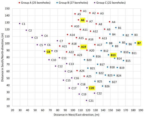
Figure 1.
Aalto New Campus Complex borehole field. Six DTS monitored boreholes are highlighted in yellow).

Table 1.
Aalto New Campus Complex BHE.
The DTS measuring equipment is introduced in Section 2.1 while the methodology for analyzing the DTS data for the estimation of borehole effective thermal resistance is presented in Section 2.3. The alternative method based on the recently developed correlations for groundwater-filled boreholes is depicted in Section 2.2. The algorithm for estimation of the effective thermal resistance of groundwater-filled boreholes has also been developed and implemented within the open-source toolbox for borehole simulation Pygfunction.
2.1. DTS Monitoring System
The distributed temperature sensing (DTS) technology has expanded significantly during the last three decades, especially utilized for continuous and accurate temperature monitoring in numerous applications of geological and subsurface processes [22], including borehole heat exchangers and their vertical temperature profiles [23,24].
Geological Survey of Finland (GTK) has installed the ANCC DTS monitoring system and is currently conducting the recording and data processing of the DTS measured data. Aalto University Campus & Real Estate (ACRE) is the owner of all data related to Aalto New Campus Complex and its energy system (including DTS data). There are six representative boreholes selected for DTS monitoring, two within each BTES group (A, B and C), namely: boreholes A6, A19, B7, B13, C8 and C20 highlighted in Figure 1.
The ANCC DTS monitoring device utilizes four channels distributed in two loops, with total cable length of 11.8 km (Figure 2). The installed DTS cable is a multimode 50 µm/125 µm fiber optic cable. There are two optic fibers in every leg of each monitoring borehole—downstream and upstream leg with bottom termination splicing. That is why fluid temperatures of each leg are measured twice and finally need to be processed by the DTS software. The DTS spatial sampling interval is 25 cm (data are taken at every 25 cm of the cable, four measurement points per meter), and even further processed for this case study. As a result, hourly based fluid temperatures have been retrieved at approx. every 10 m of the borehole depth. After proper calibration with cable coils submerged at reference temperatures, the DTS measurement accuracy is estimated around 0.1–0.5 °C.
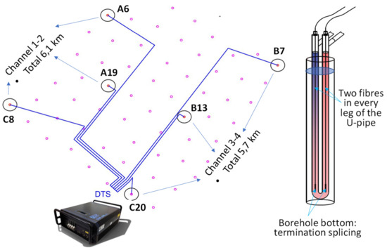
Figure 2.
Aalto New Campus Complex DTS monitoring system.
2.2. Effective Thermal Resistance of Groundwater-Filled Boreholes
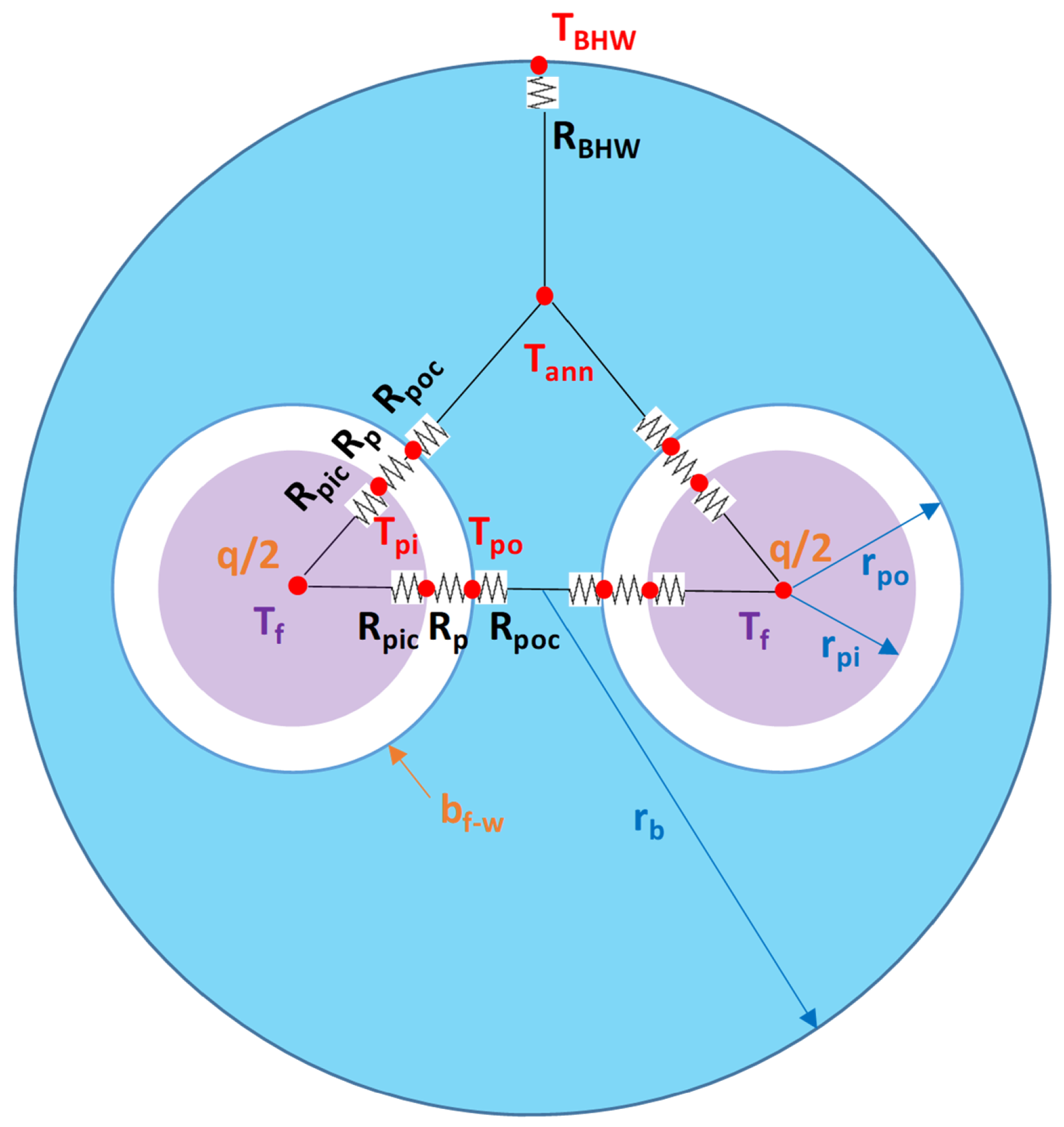
The procedure for estimating the effective thermal resistance of groundwater-filled boreholes is based on the recently developed correlations by Spitler et al. [7,25]. The methodology is summarized in the following subchapters and the procedure is developed according to the star-delta scheme depicted in Figure 3.
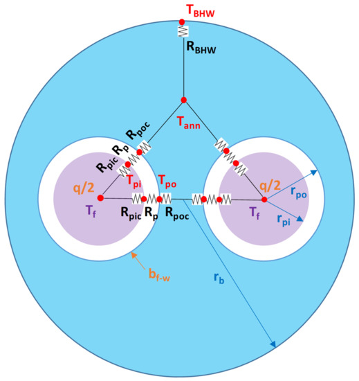
Figure 3.
Resistance scheme of groundwater-filled boreholes.
2.2.1. Convective Thermal Resistance Inside the Pipe
The internal convective resistance Rpic of the pipe depends on whether the internal flow is laminar (Reynolds number Re < 2300) or turbulent (Re ≥ 2300). It is characterized by the convective fluid-to-pipe heat transfer coefficient hpic and the Nusselt number on pipe inner wall Nupic based on the Gnielinski correlation [26]:
where Reynolds (Re) and Prandl (Pr) numbers are: , are respectively fluid velocity, density, heat capacity, dynamic viscosity and thermal conductivity; f is the pipe friction factor: .
Otherwise, the friction factor f is calculated iteratively according to the Colebrook–White equation [26].
2.2.2. Conductive Thermal Resistance of the Pipe Wall
The thermal resistance Rp of pipe wall thickness is calculated as:
where rpo, rpi and kp are respectively pipe outer/inner radius and thermal conductivity.
2.2.3. Convective Thermal Resistance at the Pipe Outer Wall
Thermal resistance Rpoc due to the natural convection of water inside the annulus is related to the heat transfer coefficient hpoc, which depends on the Rayleigh and Nusselt numbers, derived according to the following correlations [7]:
where g is the gravitational constant and kpo, νpo, αpo, and βpo are water thermal conductivity, kinematic viscosity, thermal diffusivity, and thermal expansion coefficient respectively—all evaluated at outer wall film temperature [26] calculated as the average of pipe outer surface temperature Tpo and water annulus temperature Tann; is the hydraulic diameter of the annulus space and is the heat flux at the outer pipe wall [7]; q is the heat rate per borehole depth [W/m], negative for heat extraction and positive for heat injection.
Based on real measurements of groundwater-filled boreholes, Spitler [25] suggested 124 W/m2K as a minimum value for hpoc. Additionally, water temperature at pipe outer wall can be calculated as [7]:
2.2.4. Convective Thermal Resistance at the Borehole Wall
Similarly to the convective resistance at pipe outer wall, the convective resistance RBHW at the borehole wall is related to the heat transfer coefficient hBHW, which depends on the Rayleigh and Nusselt numbers, derived according to the following correlations [7]:
where g is the gravitational constant and kBHW, νBHW, αBHW, and βBHW are water thermal conductivity, kinematic viscosity, thermal diffusivity and thermal expansion coefficient respectively—all evaluated at borehole wall film temperature [26] calculated as the average of borehole wall temperature Tpo and water annulus temperature Tann; is the hydraulic diameter of the annulus space and is the heat flux at the borehole wall [7].
Based on real measurements of groundwater-filled boreholes, Spitler [25] suggested 70 W/m2K as a minimum value for hBHW.
2.2.5. Local Thermal Resistance (Rb), Resistance between Both Legs (R12) and Total Resistance (Ra)
The local thermal resistance is defined as the resistance between the fluid of both legs of the U-pipe (symmetrical case) and the borehole wall. It takes into account the parallel connection of both legs (joining in point Tann, Figure 3) and the additional resistance at the borehole wall [7]:
Similarly, the resistance between both legs (R12) can be computed as a serial connection of all resistances between the two pipes [7]:
Borehole total resistance between the legs (Ra) is defined as [16,18]:
2.2.6. Effective Thermal Resistance (Rb*)
The effective thermal resistance characterizes the overall resistance between the fluid and the borehole wall. It determines the temperature drop between mean fluid temperature Tf (average of inlet/outlet temperatures) and borehole wall temperature Tb according to the following relation:
Depending on two different boundary conditions over the borehole – uniform borehole wall temperature (UBW) and uniform heat flux (UHF), Hellström developed the following expressions relating Rb*, Rb, R12, and Ra:
where H is the borehole depth; ρf, cf, and Vf are respectively fluid density, specific heat capacity and volume flow rate.
If r is the ratio between the effective and local thermal resistances (Rb*/Rb), finally it is possible to estimate the annulus temperature Tann as:
2.2.7. Algorithm for Calculating Rb* of Groundwater-Filled Boreholes
The calculation of Rb* is based on iterative procedure since a priori film temperatures at the annulus and borehole wall are unknown. These temperatures influence the corresponding Rayleigh and Nusselt numbers (Equations (4) and (5)) and therefore, the resulting resistances of the annulus and borehole wall. This, in turn alters the local resistance Rb (Equation (7)), the resistance between both legs R12 (Equation (8)), total resistance Ra (Equation (9)) and also Rb* (Equations (11) or (12)) depending on the adopted boundary condition mode). Finally, the iterative change in Rb* would also alter borehole wall temperature (Equation (10)) and the annulus temperature (Equation (13)). The algorithm can stop when Rb* change is small, less than a pre-established threshold.
The input parameters of the algorithm are the pumping flow rate, heat rate per meter of borehole, mean fluid temperature and the chosen boundary condition mode (UBW/UHF). The output could include some or all variables computed with Equations (1)–(13) and the calculation procedure is summarized as Algorithm 1 shown below.
| Algorithm 1. Iterative algorithm for Rb* of groundwater-filled boreholes. |
Input parameters: Pumping flow rate, heat rate per meter of borehole, mean fluid temperature, boundary condition mode (UBW/UHF)
|
2.2.8. Algorithm Implementation within Pygfunction
The presented methodology and algorithm have been implemented within the open-source toolbox for GHE simulation Pygfunction [13]. Cimmino’s versatile python application is based on the finite line source model (FLS) and can handle irregular configurations of multiple boreholes with hourly-based timestep. The applied load-aggregation schemes, like the Claesson–Javed load aggregation method [27], increase the computational speed, additionally improved in the last versions of 1.1.2 and 2.0.0 due to optimized interface for the calculation of g-functions. Cimmino has recently proposed an approximation of the FLS solution which presents adequate accuracy for simulations improving significantly the computational time [28].
Another important feature implemented in these last versions of Pygfunction is the inclusion of a new module to evaluate fluid properties using CoolProp [29]. This fluid module is directly used by the algorithm for Rb* calculation of groundwater-filled boreholes, while water properties at the pipe outer wall and borehole wall are evaluated using the external python package of IAPWS standard [30] and its _Liquid module (Properties of liquid water at 0.1 MPa).
The proposed enhancement of Pygfunction is applied with daily update of the effective thermal resistance Rb* calculated for groundwater-filled boreholes. For each timestep, the algorithm for Rb* is executed twice—for each one of the boundary conditions UBW/UHF—and finally the average of the two outcomes is taken, as suggested by Spitler and Javed [4]. The enhanced Pygfunction simulation is finally used for validation against measured fluid temperatures of the initial 39 months of system operation. It is also compared with alternative Pygfunction simulations where the value of Rb* is constant, calculated with the multipole method [31,32] for grouted boreholes used by default in Pygfunction. Root mean squared error (RMSE) is the metrics used for comparing simulation vs. measured data, defined as follows:
where N is the sample size; ym,i and ys,i are respectively the measured and simulated quantities.
2.3. Effective Thermal Resistance Derivation from DTS Measurements
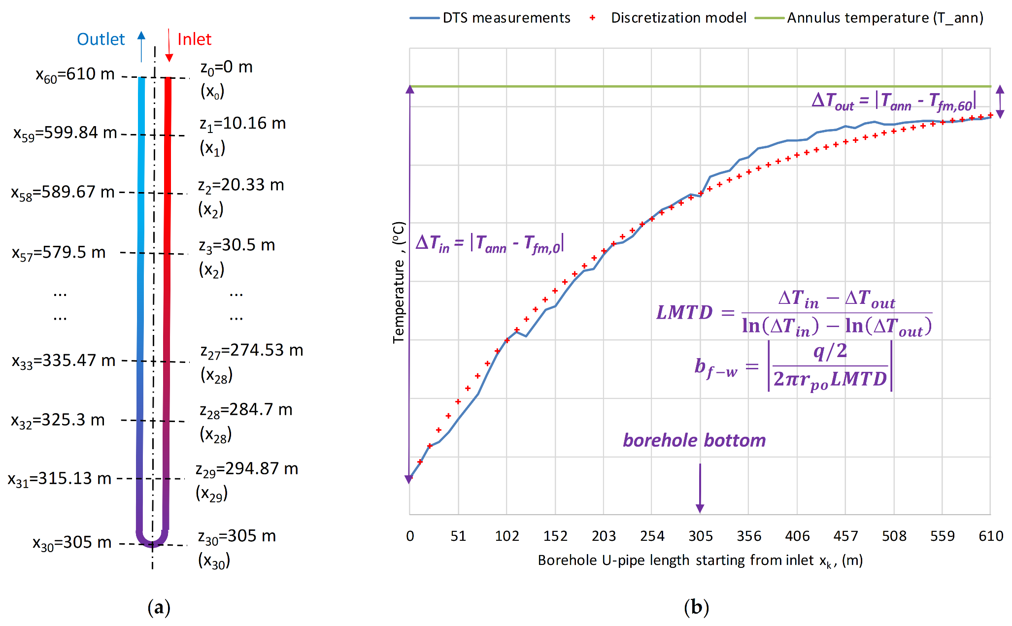
Borehole A19, a 40 mm single-U tube, 305 m depth, is selected for analyzing the DTS measured data. Fluid temperatures of both legs are taken every 10.16 m and stored every hour. As a result, there are 61 measured data points (Tfm,0, Tfm,1, Tfm,2, …, Tfm,59, Tfm,60) representing the x-axis from the borehole inlet (Tfm,0) through bottom (Tfm,30) to outlet (Tfm,60), as shown in Figure 4a. Finally, measured DTS temperatures are averaged on a daily basis, and utilized for estimating the average daily borehole effective thermal resistance (Rb*).
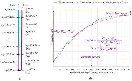
Figure 4.
DTS measurement setup of borehole A19: Vertical DTS data layout with 61 datapoints along the borehole U-pipe path (a) and discretization along the U-pipe length using LMTD and fluid-to-water heat transfer coefficient bf–w (b).
In the proposed discretization model, the borehole annulus temperature Tann is assumed to be constant over the whole borehole length. It is also assumed that the heat rate per meter of borehole (q) is evenly distributed between both legs (each leg transferring q/2). The fluid-to-water heat transfer coefficient bf–w is based on the logarithmic mean temperature difference (LMTD) between fluid and water (Figure 3 and Figure 4b) and can be derived according to the following equations:
The discretization equation of the model is based on the general equation introduced by Incropera et al. [26] (Internal flow/energy balance) for discretized fluid temperature Tf,i+1 (i = 0, 1, 2, …, 59). The model assumes that the U-pipe outer wall is maintained at constant temperature equal to the annulus temperature Tann:
The annulus temperature Tann can be determined analytically taking into account the measured fluid inlet (Tfm,0), bottom (Tfm,30) and outlet (Tfm,60) temperatures. Based on Equation (17), both downward and upward legs of the U-pipe can be characterized as follows:
Dividing Equation (18) by Equation (19), and assuming that downward and upward fluid-to-water heat transfer coefficients are equal (additional explanation regarding this assumption is provided in Appendix A), it is possible to write the following relation:
Additional constraints are established for the calculated value of Tann (Equation (20)) in order to assure the correct calculation of LMTD (Equation (15)):
- when heat is extracted (q < 0, Tfm,0 < Tfm,60), Tann should be higher than both Tfm,30 and Tfm,60
- when heat is injected (q > 0, Tfm,0 > Tfm,60), Tann should be lower than both Tfm,30 and Tfm,60
2.3.1. Derivation of the Effective Thermal Resistance
The final goal of the proposed discretization methods, introduced in the next two subchapters, is the derivation of borehole effective thermal resistance (Rb*). According to Equation (10), Rb* expresses the temperature difference between mean fluid (Tf) and borehole wall (TBHW) per unit heat flow (q). On the other hand, annulus temperature (Tann) and borehole wall (TBHW) are related in Equation (13) through the convective resistance at the borehole wall (RBHW) and the heat flow per unit depth (q). A priori, only the annulus temperature is available (calculated from Equation (20)), and the calculation steps needed to derive Rb* are summarized below:
Since the convective heat transfer coefficient at the borehole wall hBHW ≥ 70 W/m2K, the borehole wall resistance is also bounded: RBHW ≤ 0.04 m·K/W (from Equation (6)). The calculations with Algorithm 1 using A19 borehole data for 18 months (October 2019–March 2021) have confirmed that the average value of RBHW = 0.039 m·K/W, while the average value of r ratio is 1.7 and 1.8 respectively for UBW and UHR boundary condition. Therefore, a fixed value would be adopted for the term rRBHW = 0.07 m·K/W in order to derive TBHW from Tann and finally calculate Rb* (from Equation (21)). It means, in practice, that with, i.e., heat extraction rate q = −10 W/m, the temperature difference between the borehole wall and the annulus space is 0.7 °C.
2.3.2. First Discretization Method (M.1)
The proposed methodology for the calculation of annulus temperature (Equation (20)) based on three DTS measurements—fluid inlet, bottom, and outlet temperatures—will be applied in the first method. The model starts with inlet fluid temperature equal to the DTS measured inlet (initial boundary condition Tf,0 = Tfm,0) and is discretized according to Equation (17). The method is sub-divided into two alternatives (a/b):
- (a)
- the fluid-to-water heat transfer coefficient bf–w is calculated from Equation (16) and the model is discretized with Equation (17)
- (b)
- the fluid-to-water heat transfer coefficient bf–w is optimized using the method of minimization of sum of squared errors (SSE) between measured and modeled fluid temperatures (Equation (17), Figure 4b), the optimization model is formulated as follows:
The optimization problem is solved using the Generalized Reduced Gradient (GRG) non-linear method of MS Excel Solver (on a daily basis).
2.3.3. Second Discretization Method (M.2)
The second method is based on Hellström’s vertical profile (for uniform borehole wall temperature), additionally developed by Lamarche et al. [18]. In this second approach, previously derived borehole wall temperature TBHW (based on the calculated annulus temperature Tann from Equation (20), and borehole wall temperature TBHW from Equation (21)) is used for the calculation of the vertical profile defined as follows:
where is the relative depth within the borehole, η is the parameter already defined in Equation (11) which can be equivalently related with resistances Ra and Rb below:
and parameters ξ and ζ are defined as follows:
Downward and upward legs fluid temperatures Tf,z (Equations (23) and (24)) are discretized at points z=z1, z2, …, z30 (Figure 4a) taking as inlet the DTS measured inlet fluid temperature (Tf,0 =Tfm,0). Both resistances Ra and Rb are optimized using the method of SSE minimization between measured and modeled fluid temperatures (Equations (23)–(26)). The optimization model is formulated below:
The optimization problem is solved using the GRG non-linear method of MS Excel Solver (on a daily basis). The final goal is the derivation of borehole effective thermal resistance Rb*, which can be done using Equation (25) (based on Rb and η).
3. Results
The results presented in this section include the analysis of the A19 borehole DTS measured data within the period October 2019–March 2021. This analysis is used for deriving the effective thermal resistance of borehole A19 on a daily basis and comparing the results with the algorithmic procedure based on Spitler’s correlations for groundwater-filled boreholes.
Additionally, the proposed algorithm for the effective thermal resistance of groundwater-filled boreholes (Rb*) is coupled with the Pygfunction toolbox (with daily update of Rb*) and utilized for validation against measured fluid temperatures of the initial 39 months of system operation (March 2018–May 2021).
3.1. Borehole A19 Data Analysis and Effective Thermal Resistance
Data are taken on a daily basis: fluid temperatures from the DTS measurements and pumping flow rates taken from previous research [21] (assuming that total pumping is evenly distributed among the boreholes. The most relevant variables of borehole A19 are summarized in Table 2 and Table 3.
Table 2.
Borehole A19 (DTS data analysis). Comparison of Methods 1 (a/b) and 2.
Table 3.
Borehole A19. Comparison of Methods 1 (a/b), 2 and the Algorithm for Rb* calculation (UBW/UHR).
Winter operation is characterized with significant heat extraction from November to April (from −12 to −18 W/m) and higher pumping flow rates (0.4–0.5 l/s), while summer period is short, mostly comprising only 3 months (June, July, and August). September is almost neutral (heat extraction roughly equals injection) reflected in its lower LMTD and fluid-to-water heat transfer coefficient bf–w. On the other hand, typical winter months present higher LMTD close to 1 (0.9–1.1 °C) and higher fluid-to-water heat transfer coefficient bf–w (65–75 W/m2K). Winter months are also easier to fit to DTS measured data, as reflected in their lower SSE values (0.1–0.5 K2). Overall, the second method is the most accurate and capable to fit extremely well to DTS measurements, reflected on its lowest SSE.
The average internal resistance Ra obtained with method 2 (0.26 m·K/W) is slightly higher than the outcome of the algorithm with UBW (0.19 m·K/W), values in line with 0.32 m·K/W calculated with the first-order multipole method [4,33] for grouted borehole (assuming grout thermal conductivity kg = 1.2 W/mK). The same is valid when comparing the average local resistance Rb: 0.15, 0.12, and 0.09 m·K/W respectively with method 2, algorithm with UBW and the first-order multipole [4,33]; however it is compensated by the parameter η (1.38 vs. 1.58), and finally all outcomes for Rb* are very similar over the whole 18-month-long period (Table 3).
Good agreement can be acknowledged between all methods and the algorithm: the annual 2020 average Rb* is 0.20–0.22 m·K/W with higher values during the summer months. The winter–summer dichotomy is reflected in lower winter effective thermal resistance Rb* (0.14–0.17 m·K/W) while in summer the monthly values of Rb* can rise to 0.24–0.36 m·K/W. The latter is also related to the dominant days with laminar flow within the U-pipe from June to October 2020 due to the lower pumping flow rate, also reported by Spitler and Javed [4].
More detailed weekly-averaged values of Rb* and pumping flow rate are plotted in Figure 5, both methods (1 and 2) and the algorithmic solution (with two boundary conditions UBW and UHF, the former presenting slightly lower values compared with the latter as shown in [4]). There is a good agreement in winter operation with all options in a compact band (especially coinciding the different calculation approaches in methods 1 and 2). In summer operation, Rb* values are more dispersed with frequent ups and downs, with some extreme values provided by method 2, indicating higher uncertainty with lower heat and pumping flow rates (Figure 5).
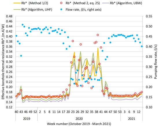
Figure 5.
A19 borehole weekly effective thermal resistance and flow rate.
3.2. Graphical Analysis of Discretization Methods 1 and 2
In order to illustrate how well the different discretization methods work (borehole A19), two different charts are plotted on a monthly basis:
- (a)
- three months with dominating heat extraction typical for winter operation—February, April, and November 2020
- (b)
- one month with dominating heat injection typical for summer operation—August 2020, and two intermediate months—May/September 2020
3.2.1. Borehole A19 (Method 1a)
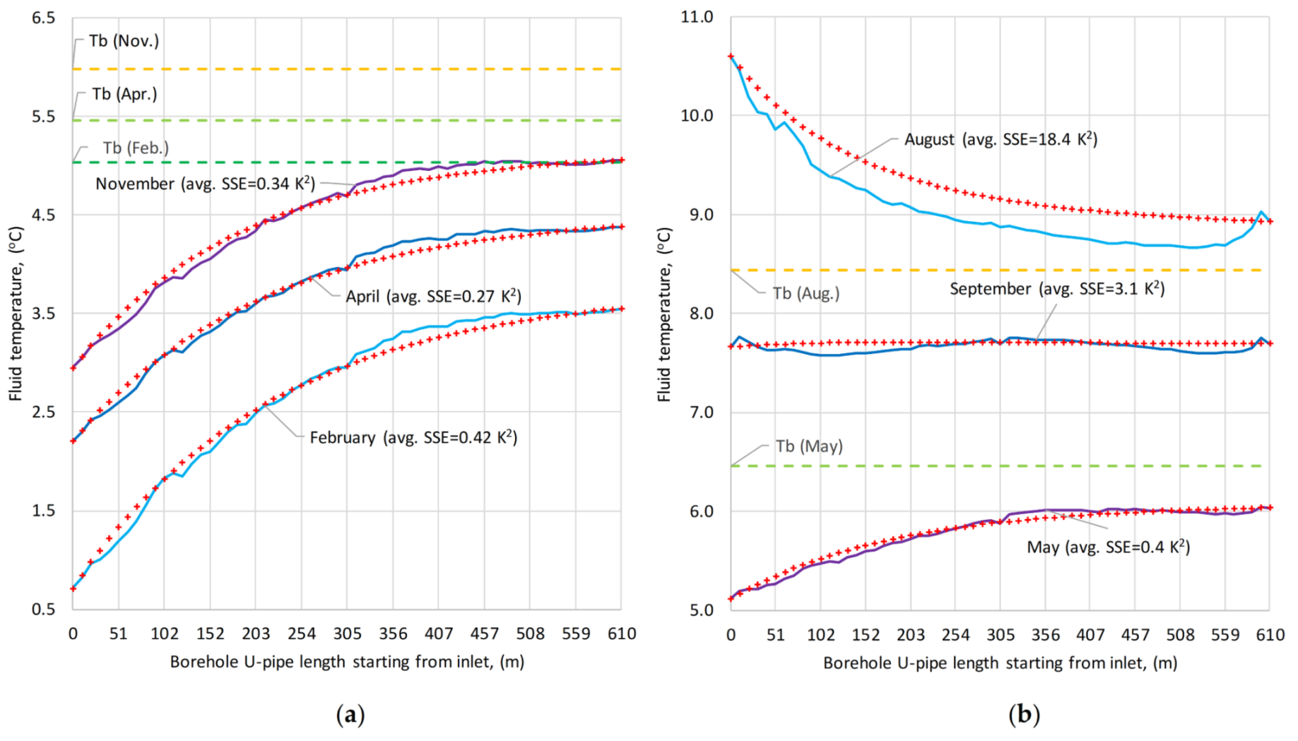
The corresponding chart comparing DTS measurements (thick curves) vs. discretization method 1a is plotted in Figure 6.

Figure 6.
Graphical representation of discretization method 1a (red cruxes) vs. DTS measurements. Winter operation with dominant heat extraction (a). Summer (heat injection) and intermediate operation (b). Temperatures at the borehole wall (Tb) are also shown as reference.
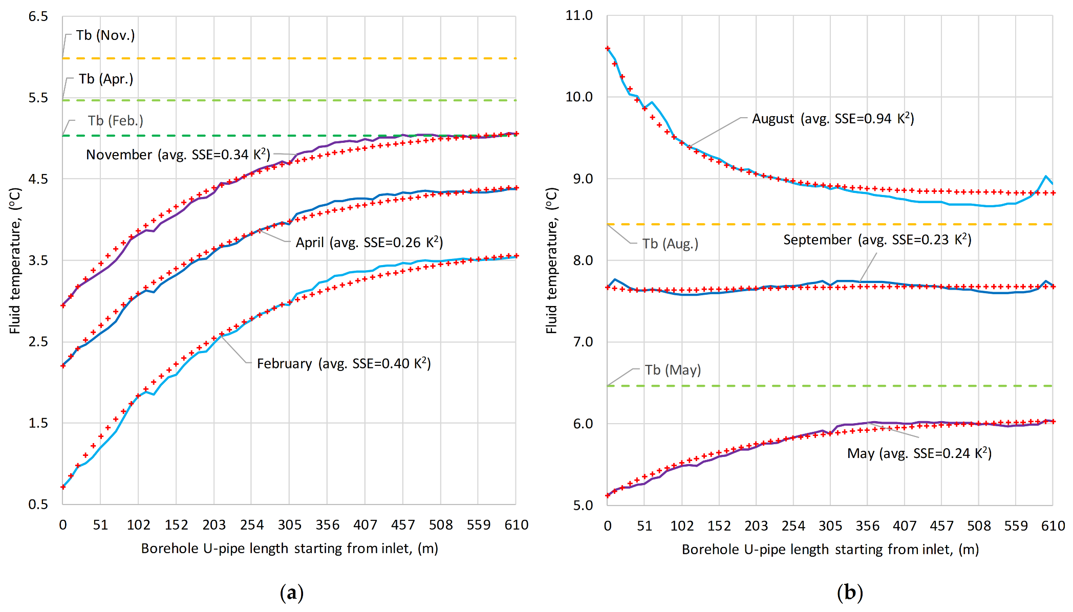
3.2.2. Borehole A19 (Method 1b)
The corresponding chart comparing DTS measurements (thick curves) vs. discretization method 1b is plotted in Figure 7. The average monthly SSE’s show improvement in summer operation (Figure 7b) compared with method 1a.
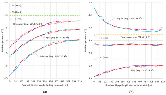
Figure 7.
Graphical representation of discretization method 1b (red cruxes) vs. DTS measurements. Winter operation with dominant heat extraction (a). Summer (heat injection) and intermediate operation (b). Temperatures at the borehole wall (Tb) are also shown as reference.
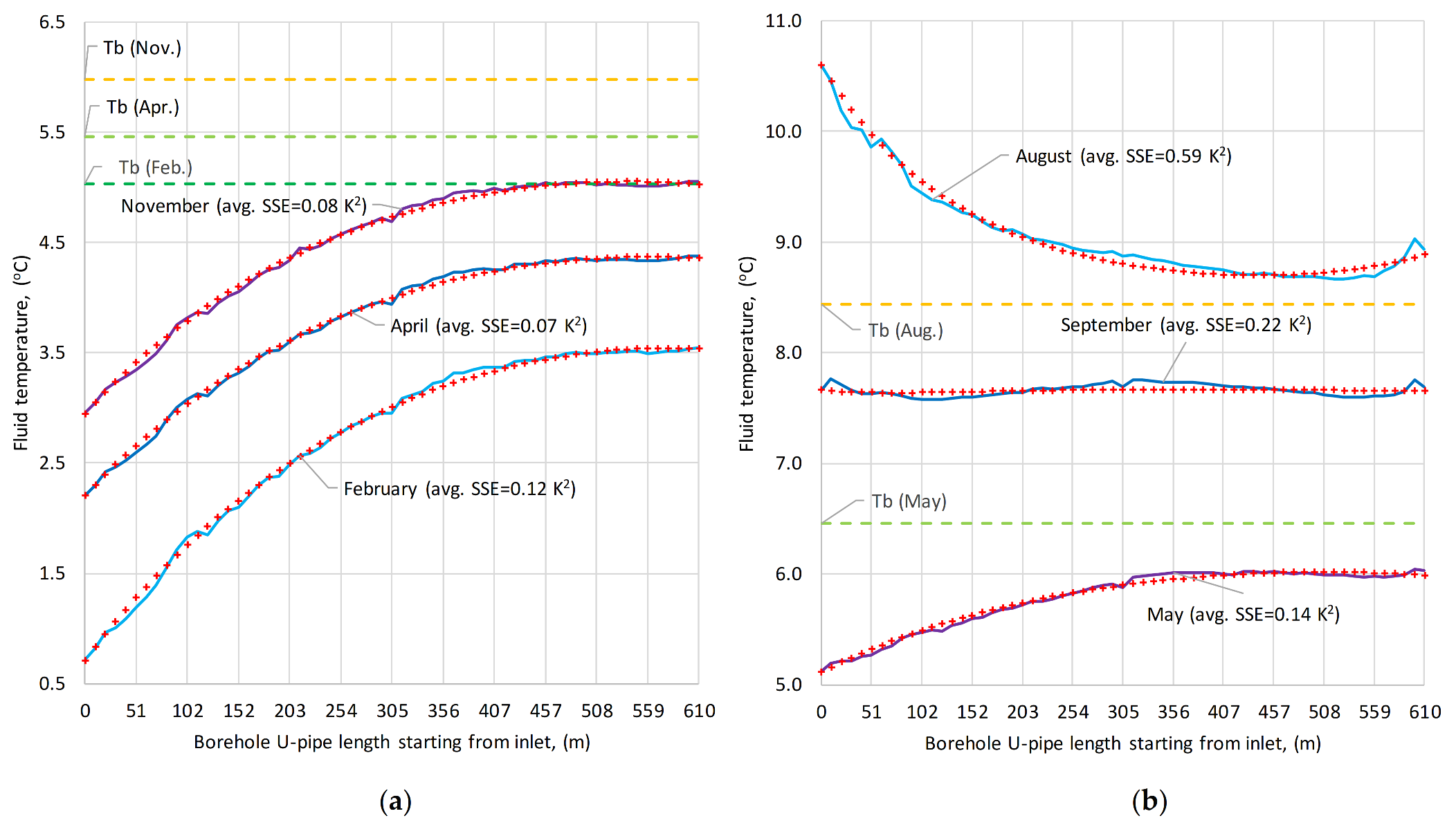
3.2.3. Borehole A19 (Method 2)
The corresponding chart comparing DTS measurements (thick curves) vs. discretization method 2 is plotted in Figure 8. The average monthly SSE’s show significant improvement for all months compared with method 1. This can be acknowledged especially in August when the discretization curve fits very accurately the DTS measurements, despite the significant short-circuiting between borehole legs. This can be seen in Figure 8b as the upward leg (right part, 305–610 m) is gaining heat from the downward one before reaching the outlet. This is a confirmation that the quasi-three-dimensional vertical temperature profile [14,18] can effectively account for a thermal short-circuiting between both legs [34], especially exacerbated with low pumping flow rates and deep boreholes over 200 m [35].
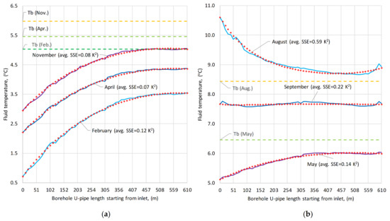
Figure 8.
Graphical representation of discretization method 2 (red cruxes) vs. DTS measurements. Winter operation with dominant heat extraction (a). Summer (heat injection) and intermediate operation (b). Temperatures at the borehole wall (Tb) are also shown as reference.
3.3. Model Validation: Initial 39 Months of System Operation
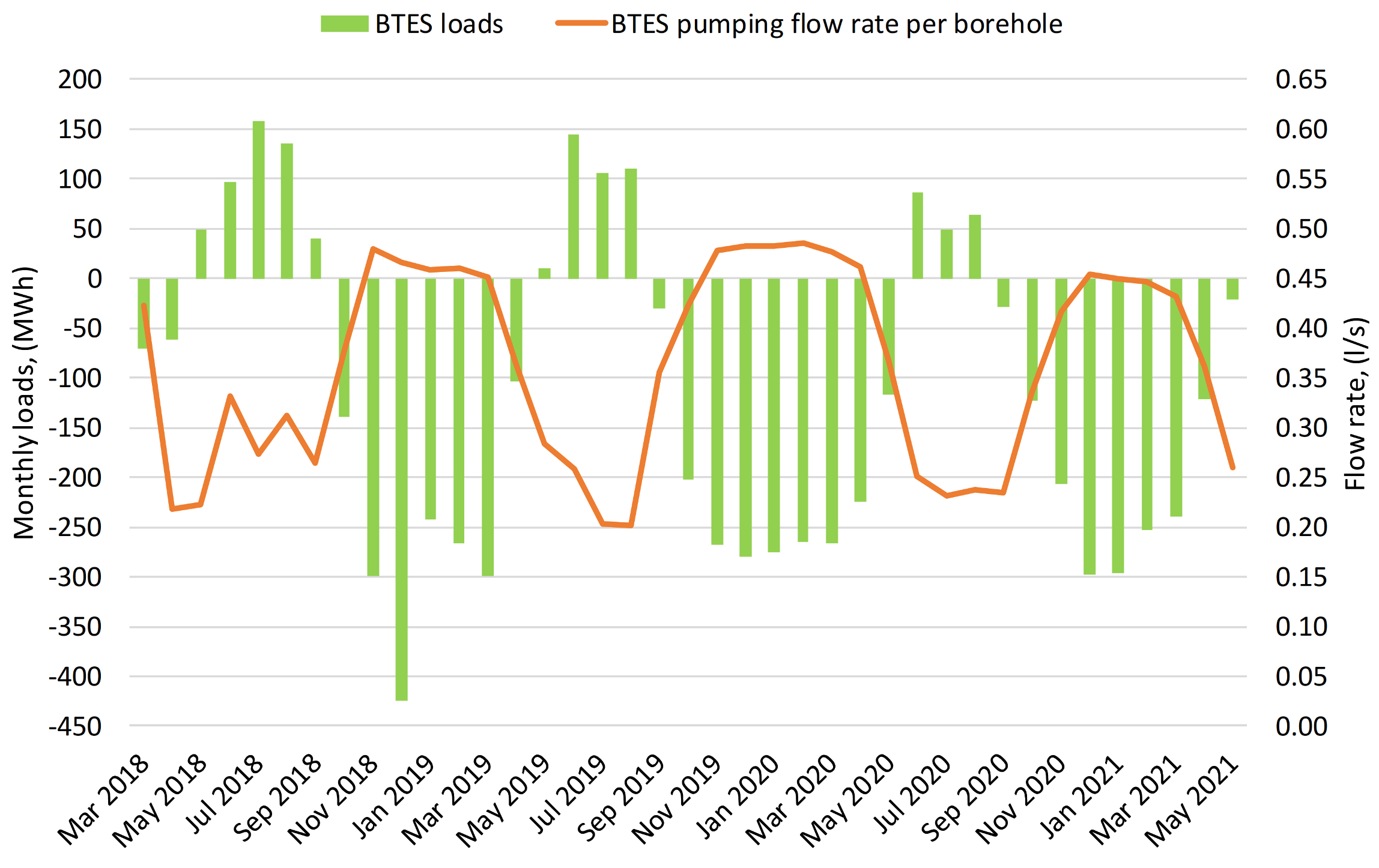
The DTS monitoring system has been operating since 7 February 2019. However, there are temperature measurements of the BTES circuit (inlet/outlet temperatures) since around the middle of March 2018 as well as overall GSHP/circulation pumps (CP) activity. Following the methodology for data reconstruction proposed by Todorov et al. [21], it is possible to establish the following correlations between the pumping volume flow rate Vf (in l/s per borehole) and the frequency percentage signals (FP1/FP2) sent to each one of the twin CP (BTES field):
The BTES loads between October 2019 and May 2021 are obtained using the specifically developed data validation and reconciliation (DVR) methodology [21]. Prior to this, BTES loads are estimated based on the pumping flow rates (linear regression, Equation (28)) and measured inlet/outlet BTES temperatures. Resulting BTES loads and pumping flow rates (on a monthly basis) are shown in Figure 9.
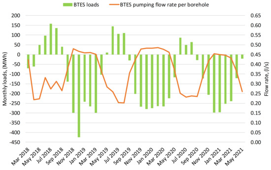
Figure 9.
BTES loads and pumping flow rates (2018–2021).
The developed models utilize daily-based data (loads and pumping flows), borehole field geometry and ground parameters according to Table 1. The different scenarios are listed below:
- Measured data (mean fluid temperature)
- Simulated: Algorithm for Rb* calculation of water-filled boreholes coupled with Pygfunction (with daily Rb* update, average Rb* = 0.22 m·K/W)
- Simulated: Pygfunction modeling standard grouted boreholes, grout thermal conductivity kg = 0.6 W/mK (constant Rb* = 0.18 m·K/W)
- Simulated: Pygfunction modeling standard grouted boreholes, grout thermal conductivity kg = 1.2 W/mK (constant Rb* = 0.13 m·K/W)
- Simulated: Pygfunction modeling standard grouted boreholes, grout thermal conductivity kg = 1.8 W/mK (constant Rb* = 0.12 m·K/W)
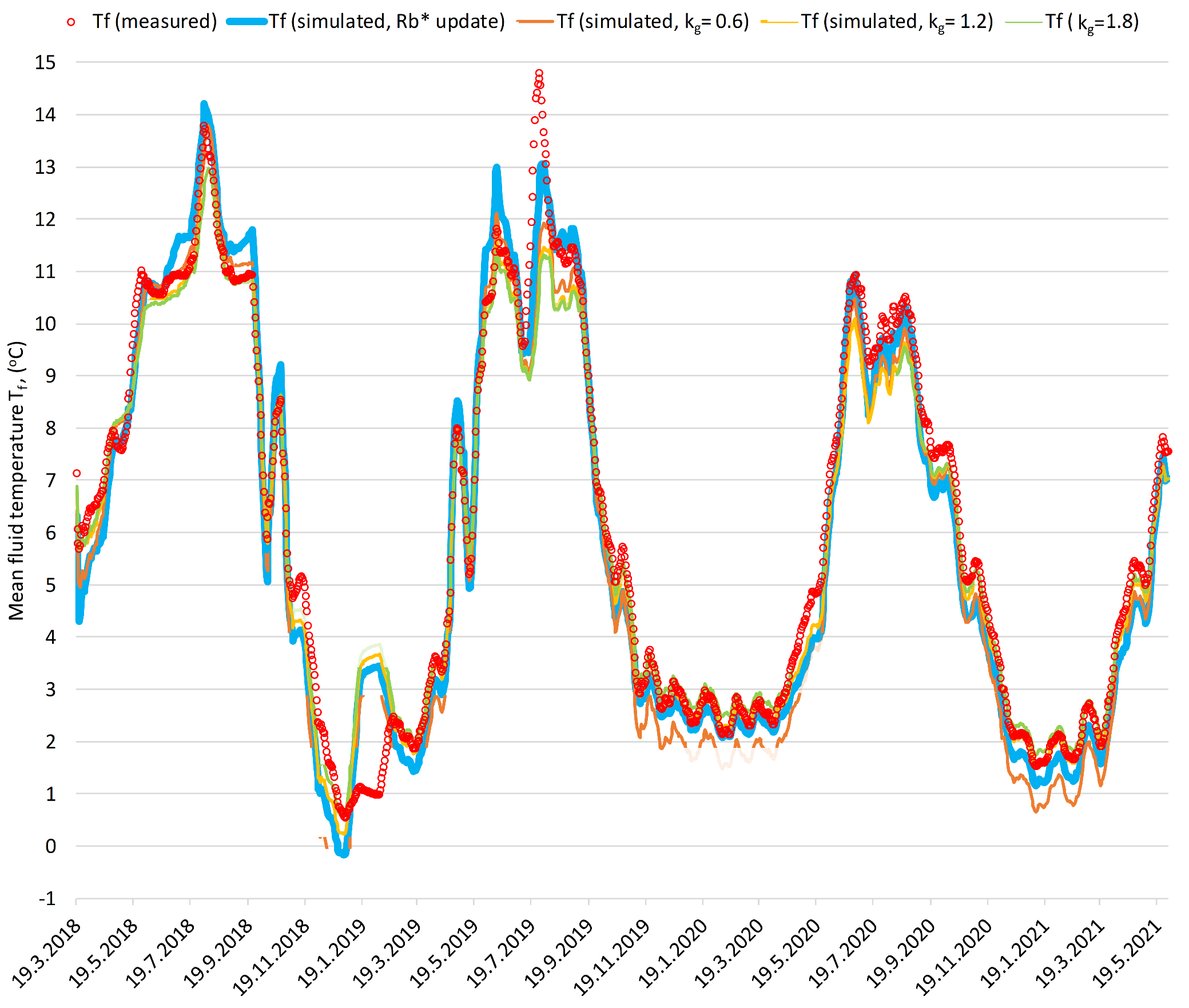
The results, using a 15-day moving average of the mean fluid temperature, in order to reduce the noise in data representation, are plotted in Figure 10.

Figure 10.
Model validation: measured mean fluid temperature vs. simulations.
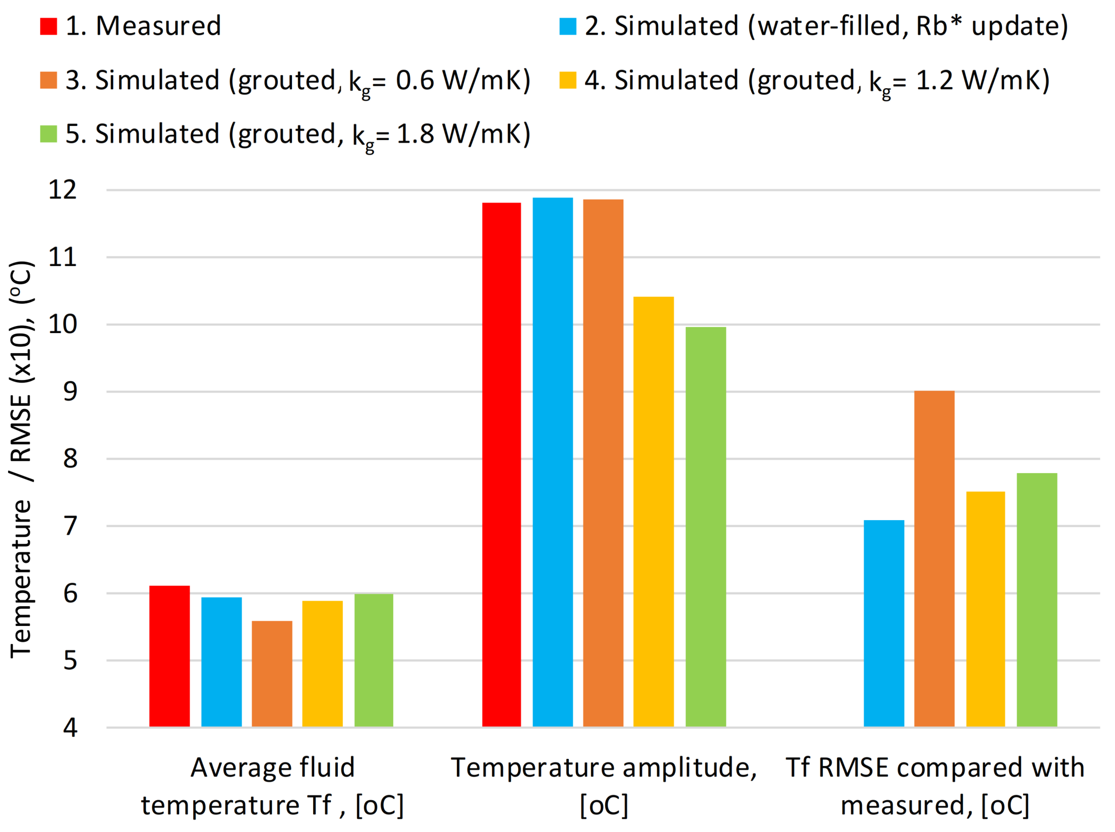
The annual comparison metrics, developed as 365-day periods after the starting day (19 March 2018) are summarized below:
- Mean fluid temperature (annual and overall average)
- Temperature amplitude, difference between maximum and minimum fluid temperatures within the annual period (annual and overall average)
- Mean fluid temperature RMSE, compared with measurements (annually and overall)
Table 4.
Model validation: results comparison.
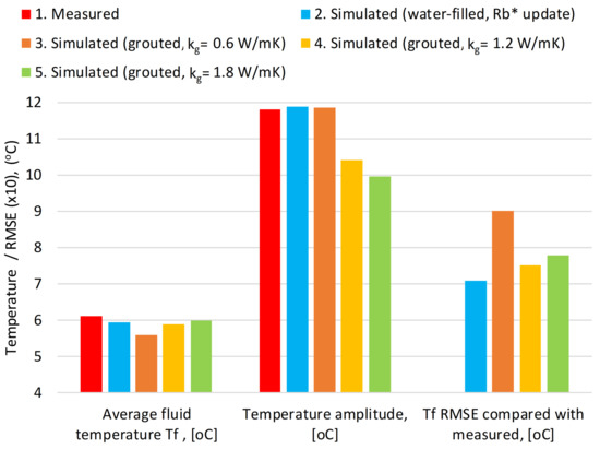
Figure 11.
Model validation: overall comparison indicators.
4. Discussion
All methods using DTS data analysis of borehole A19 for the estimation of the effective thermal resistance (Rb*) show good agreement with the algorithm based on correlations. It is interesting to acknowledge that in summer operation (normally associated with lower pumping flow rate below 0.3 l/s), the Rb* values are more dispersed (Figure 5), while in winter they form a more compact block where both algorithm boundary conditions (UBW/UHR) give lower outcome than the discretization methods 1 and 2. Moreover, both methods (1 and 2) fit more accurately the DTS measured profiles during the winter operation, clearly reflected in the lower average SSE values below 0.5 K2 (Table 2).
On the other hand, method 1a handles very poorly summer operation with SSE over 18 K2 in August, compared with 0.9–1.4 K2 in method 1b and 0.4–1 K2 in method 2, clearly seen in Figure 6b (the discretization curve is not flexible enough to fit well the measured data). Overall, the fluid-to-water heat transfer coefficients bf–w tend to increase when the absolute heat load q increase, i.e., in winter operation when the heat extraction is high. In this respect, September with near 0 heat rate, is presenting a challenging DTS profile with several ups and downs (Figure 6). Furthermore, the bf–w optimization in method 1b, brings a clear advantage for fitting the DTS measurements in summer operation (Table 2, Figure 7 and Figure 8). Method 2, utilizing Hellström’s vertical profile formulation, is the most accurate since it takes into account the short-circuiting between the legs (i.e., DTS curve swing in August indicates this, a temperature short-circuiting due to lower pumping flow rate). Therefore, it can be adapted more precisely to measured data (Figure 8).
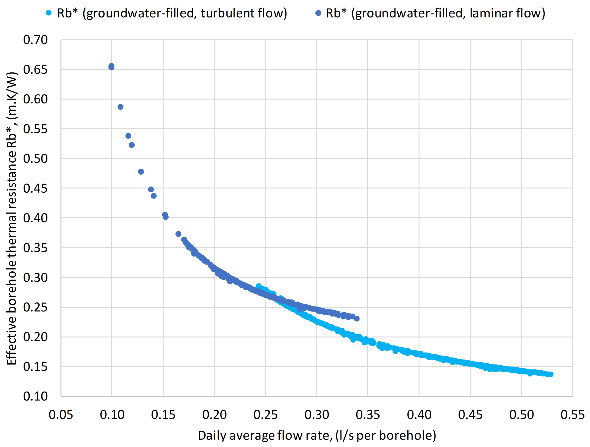
The correlation of Rb* with the pumping flow rate, noticed already in Figure 5, is definitely confirmed when plotting data of the validation model over the whole 39-month-long period with daily resolution (Figure 12).
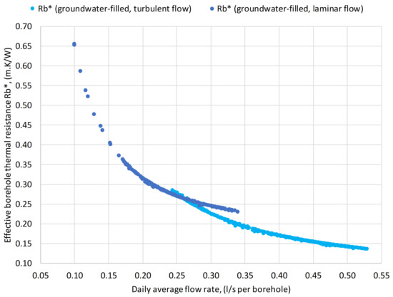
Figure 12.
Effective thermal resistance of groundwater-filled boreholes vs. flow rate.
Among all these 1170 days (from 19 March 2018 to 31 May 2021), the flow is laminar some 30% of the time, mostly during summer operation as previously shown in Table 3 (borehole A19). Laminar flow regime inside the U-pipe (Re < 2300) can provoke a steeper exponential increase of daily Rb* up to 0.66 m·K/W (Figure 12). On the other hand, minimum flow rates in the range of 0.25–0.35 l/s per borehole can assure a turbulent regime (Re ≥ 2300) and lower values for Rb*. Moreover, it is acknowledged a significant variability of Rb* in real operation, considering that the initial TRT results estimated Rb* slightly below 0.1 m·K/W. Lower flow rate (laminar flow within the U-pipe) increases the thermal short-circuiting between both legs, rises the effective borehole thermal resistance and ultimately degrades the overall efficiency of the GHE [4,35].
The presented hybrid model, enhancing the Pygfunction toolbox with capabilities to calculate the Rb* of water-filled boreholes dynamically and updating it during the simulation, has shown very good agreement with measured data (Figure 10), even though the uncertainty of the estimation of BTES loads and flow rates before October 2019 is high. The model fits closely the measured data, which is reflected on its best comparison indicators: average fluid temperature, temperature amplitude of the annual cycle and RMSE (Figure 11). It is followed by the Pygfunction simulation with grout thermal conductivity kg = 1.2 W/mK (and constant Rb* = 0.13 m·K/W), however the latter differs in temperature amplitude which is reflected in its difficulty to follow the measured data curve during the summer peaks (Figure 10). Similar value for grout thermal conductivity (kg = 1.3 W/mK) is also suggested by Earth Energy Designer (EED) [36] when simulating groundwater-filled boreholes [37]. The only significant deviation between measurements and simulation occurs between 13 and 23 July 2019 (Figure 10) when the BTES circulation pumps had very low activity (stopping completely for 53 h) and the mean fluid temperature increased approaching the ambient temperature.
Aalto New Campus Complex is an extreme case of heating dominated system [21] and characterized with significant heat imbalance of the GSHP-BTES interactions (net annual heat extraction 1.2–1.7 GWh). Considering scenarios 3, 4, and 5 (with constant Rb*), as Rb* decreases (by improving the thermal conductivity of the backfilling material kg), the temperature amplitude also decreases, and the overall mean fluid temperature path does not decline so rapidly as seen in Table 4 and Figure 11 (average fluid temperature). This is a similar conclusion also highlighted by Marcotte and Pasquier [38]. That is why, it is so important to maintain Rb* as low as possible, for efficient and sustainable long-term operation [4].
5. Conclusions
The presented case study introduced several approaches for determining the effective thermal resistance Rb* of groundwater-filled boreholes. The proposed two methods utilized the DTS temperature profile of one representative borehole of the irregular BTES field (A19), derived the borehole annulus temperature based on fluid inlet, bottom, and outlet temperatures and introduced different methodologies for discretizing and modeling the vertical profile in order to fit the DTS measurements. The first method estimates the fluid-water LMTD and the fluid-to-water heat transfer coefficient. Its discretization is based on the general approach for internal flow proposed by Incropera et al. [26]. The second method utilizes the borehole wall temperature (determined indirectly from borehole annulus temperature) and is based on Hellström’s formulation of borehole vertical profile developed by Lamarche et al. [18]. The final goal of both methods is the derivation of Rb*.
The second approach of the present research utilizes the recently developed correlations for groundwater-filled boreholes proposed by Spitler et al. [7,25]. The resulting algorithm for the effective thermal resistance Rb* of groundwater-filled boreholes is implemented within the python-based toolbox for GHE simulation Pygfunction (Cimmino [13]). Both methods and the implemented algorithm have presented good agreement in the results of Rb* estimation, analyzing the 18-month DTS measurements of borehole A19. Overall, Lamarche’s approach based on Hellström’s formulation achieved the highest accuracy for mimicking the DTS measured profiles even in challenging situations with short-circuiting between borehole legs.
Finally, a simulation of the initial 39-months of system operation is conducted with Pygfunction and validated against measured data. One of the simulation scenarios is a hybrid model between Pygfunction and the algorithm implementation for groundwater-filled boreholes, updating Rb* on a daily basis. The other three scenarios used grouted boreholes with specified grout thermal conductivity and constant borehole thermal resistance over the entire simulation.
Overall, the hybrid model (with daily Rb* update) presented the best indicators and fitted well with measurements. Therefore, it is concluded that the specifically developed algorithm for calculating the Rb* of groundwater-filled boreholes is essential for a reliable long-term simulation. Additionally, a suboptimal operation of the BTES circulation pumps is detected, with some 30% of the days operating in laminar flow regime (mostly in summer), provoking a steeper exponential increase of the effective borehole thermal resistance. The implementation of strategy for minimum pumping flow rate is recommended in order to assure turbulent regime within the borehole U-pipe and lower borehole effective thermal resistance. Furthermore, DTS measurements of groundwater temperature along the annulus space and the borehole wall (in addition to fluid temperature) are also recommendable since they are essential for improving the confidence and accuracy of the results.
Author Contributions
Conceptualization, O.T.; methodology, O.T.; software, O.T.; validation, O.T.; formal analysis, O.T.; investigation, O.T.; resources, O.T. and K.A.; data curation, O.T.; writing—original draft preparation, O.T.; writing—review and editing, O.T. and K.A.; visualization, O.T.; supervision, R.K.; project administration, M.V.; funding acquisition, R.K. and M.V. All authors have read and agreed to the published version of the manuscript.
Funding
This research was funded by Business Finland, grant number 8199/31/2018.
Institutional Review Board Statement
Not applicable.
Informed Consent Statement
Not applicable.
Data Availability Statement
The data are not publicly available due to a confidentiality agreement with Aalto University Campus & Real Estate (ACRE).
Acknowledgments
This research is part of the Smart Otaniemi Project (Aalto University) and contribution to the IEA HPT Annex 52, “Long term performance measurement of GSHP systems serving commercial, institutional, and multi-family buildings”. We highly appreciate the support of M. Cimmino, A.M. Gustafsson, J. Johnsson and J. D. Spitler. We wish to thank A. Säynäjoki from Aalto University Campus & Real Estate as well as N. Leppäharju and S. Vallin from the Geological Survey of Finland.
Conflicts of Interest
The authors declare no conflict of interest.
Abbreviations
| ACRE | Aalto University Campus & Real Estate |
| ANCC | Aalto New Campus Complex |
| BHE | Borehole Heat Exchanger |
| BTES | Borehole Thermal Energy Storage |
| CFF | Combined Frequency Factor |
| CP | Circulation Pump |
| COP | Coefficient of Performance |
| DVR | Data Validation and Reconciliation |
| DTS | Data Temperature Sensing |
| FLS | Finite Line Source model |
| EED | Earth Energy Designer |
| EFT | Entering Fluid Temperature (GSHP evaporator) |
| GHE | Ground Heat Exchanger |
| GRG | Generalized Reduced Gradient |
| GTK | Geological Survey of Finland |
| GSHP | Ground Source Heat Pump |
| LMTD | Logarithmic Mean Temperature Difference |
| RMSE | Root Mean Squared Error |
| SSE | Sum of squared errors |
| TRT | Thermal Response Test |
| UBW | Uniform Borehole Wall temperature |
| UHF | Uniform Heat Flux |
| bf–w | Fluid-to-water heat transfer coefficient, [W/m2K] |
| bf–w,down | Fluid-to-water heat transfer coefficient downward leg, [W/m2K] |
| bf–w,up | Fluid-to-water heat transfer coefficient upward leg, [W/m2K] |
| cf | Mean fluid heat capacity, [J/kg·K] |
| DH | Hydraulic diameter of the borehole annulus, [m] |
| f | Friction factor |
| g | Gravitational constant, [m2/s] |
| H | Borehole depth, [m] |
| hpic | Convective fluid-to-pipe heat transfer coefficient, [W/m2K] |
| hpoc | Convective heat transfer coefficient at the outer pipe wall, [W/m2K] |
| hBHW | Convective heat transfer coefficient at the borehole wall, [W/m2K] |
| kf | Mean fluid thermal conductivity, [W/m·K] |
| kg | Grout thermal conductivity, [W/m·K] |
| kp | Pipe wall thermal conductivity, [W/m·K] |
| kpo | Water thermal conductivity at pipe outer wall, [W/m·K] |
| kBHW | Water thermal conductivity at the borehole wall, [W/m·K] |
| Nupo | Water Nusselt number at pipe outer wall |
| NuBHW | Water Nusselt number at the borehole wall |
| Pr | Prandtl number |
| q | Heat rate per borehole depth, [W/m] |
| q”po | Heat flux at the outer pipe, [W/m2] |
| q”BHW | Heat flux at the borehole wall, [W/m2] |
| Rapo | Water Rayleigh number at pipe outer wall |
| RaBHW | Water Rayleigh number at the borehole wall |
| Re | Reynolds number |
| Rpic | Convective resistance at pipe inner wall, [m·K/W] |
| Rpc | Pipe wall conductive resistance, [m·K/W] |
| Rpoc | Convective resistance at pipe outer wall, [m·K/W] |
| R12 | Thermal resistance between both U-pipe legs, [m·K/W] |
| Ra | Borehole total thermal resistance, [m·K/W] |
| Rb | Borehole local thermal resistance, [m·K/W] |
| Rb* | Borehole effective thermal resistance, [m·K/W] |
| r | Ratio between borehole effective and local thermal resistances |
| rb | Borehole radius, [m] |
| rpi | Pipe inner radius, [m] |
| rpo | Pipe outer radius, [m] |
| Tann | Annulus temperature, [°C] |
| TBHW, Tb | Temperature at the borehole wall, [°C] |
| Tf, Tfm | Mean fluid temperature, [°C] |
| Tf,i | Modeled (discretized) fluid temperature, i = 0, 1, …, 60 [°C] |
| Tf,z | Modeled (method 2) fluid temperature, [°C] |
| Tfm,i | DTS measured fluid temperature, i = 0, 1,…, 60 [°C] |
| Tpi | Temperature at the pipe inner wall, [°C] |
| Tpo | Temperature at the pipe outer wall, [°C] |
| Uf | Mean fluid velocity, [m/s] |
| Vf | Mean fluid volume flow rate, [m3/s] |
| αpo | Water thermal diffusivity at pipe outer wall, [m2/s] |
| αBHW | Water thermal diffusivity at the borehole wall, [m2/s] |
| βpo | Water thermal expansion coefficient at pipe outer wall, [1/K] |
| βBHW | Water thermal expansion coefficient at the borehole wall, [1/K] |
| ζ | Parameter of vertical profile model (Lamarche/Hellström) |
| η | Parameter of vertical profile model (Lamarche/Hellström) |
| μf | Mean fluid dynamic viscosity, [Pa.s] |
| νpo | Water kinematic viscosity at pipe outer wall, [m2/s] |
| νBHW | Water kinematic viscosity at the borehole wall, [m2/s] |
| ξ | Parameter of vertical profile model (Lamarche/Hellström) |
| ρf | Mean fluid density, [kg/m3] |
Appendix A
Below is presented the exponential analytical solution provided by Incropera et al. [26], applied for the estimation of borehole fluid axial temperature distribution Tx at a distance x (0 ≤ x ≤ 2H) of the U-pipe exposed to a constant temperature Tann (borehole water annulus temperature), with inlet fluid temperature T0 and fluid-to-water heat transfer coefficient bf–w:
Considering a segment of the pipe with length Δx (between x and x + Δx), at point x + Δx Equation (A1) yields:
The discretization at point x + Δx from the previous point x can be written accounting for the local fluid-to-water heat transfer coefficient bf–w,Δx (dependent on the segment length Δx):
Equation (A3) shows that bf–w,Δx depends only on Δx (not depending on the relative position x within the pipe). That is why, if we consider both legs of the U-pipe with length Δx = H, both downward and upward local fluid-to-water heat transfer coefficients would be equal.
References
- Net Zero by 2050: A Roadmap for the Global Energy Sector, International Energy Agency (Special Report). Available online: https://iea.blob.core.windows.net/assets/4719e321-6d3d-41a2-bd6b-461ad2f850a8/NetZeroby2050-ARoadmapfortheGlobalEnergySector.pdf (accessed on 23 August 2021).
- Todorov, O.; Alanne, K.; Virtanen, M.; Kosonen, R. Aquifer thermal energy storage (ATES) for district heating and cooling: A novel modeling approach applied in a case study of a Finnish urban district. Energies 2020, 13, 2478. [Google Scholar] [CrossRef]
- Spitler, J.D.; Gehlin, S.E.A. Thermal response testing for ground source heat pump systems—An historical review. Renew. Sustain. Energy Rev. 2015, 50, 1125–1137. [Google Scholar] [CrossRef]
- Javed, S.; Spitler, J.D. Calculation of Borehole Thermal Resistance; Woodhead Publishing: Cambridge, UK, 2016; Volume 1, ISBN 9780081003220. [Google Scholar]
- Javed, S.; Nakos, H.; Claesson, J. A method to evaluate thermal response tests on groundwater-filled boreholes. ASHRAE Trans. 2012, 118, 540–549. [Google Scholar]
- Gustafsson, A.M.; Westerlund, L. Heat extraction thermal response test in groundwater-filled borehole heat exchanger—Investigation of the borehole thermal resistance. Renew. Energy 2011, 36, 2388–2394. [Google Scholar] [CrossRef]
- Spitler, J.D.; Javed, S.; Ramstad, R.K. Natural convection in groundwater-filled boreholes used as ground heat exchangers. Appl. Energy 2016, 164, 352–365. [Google Scholar] [CrossRef]
- Liebel, H.T.; Javed, S.; Vistnes, G. Multi-injection rate thermal response test with forced convection in a groundwater-filled borehole in hard rock. Renew. Energy 2012, 48, 263–268. [Google Scholar] [CrossRef] [Green Version]
- José, A. Distributed Thermal Response Tests—New Insights on U-Pipe and Coaxial Heat Exchangers in Groundwater-Filled Boreholes. Ph.D. Thesis, KTH Royal Institute of Technology, Stockholm, Sweden, 2013. [Google Scholar]
- Gustafsson, A.M.; Gehlin, S. Influence of natural convection in water-filled boreholes for GCHP. ASHRAE Trans. 2008, 114, 416. [Google Scholar]
- Javed, S.; Spitler, J.D.; Fahlen, P. An experimental investigation of the accuracy of thermal response tests used to measure ground thermal properties. ASHRAE Trans. 2011, 117, 13–21. [Google Scholar]
- Johnsson, J.; Adl-Zarrabi, B. Modelling and evaluation of groundwater filled boreholes subjected to natural convection. Appl. Energy 2019, 253, 113555. [Google Scholar] [CrossRef]
- Cimmino, M.; Thorne, D.; Langevin, C.D.; Sukop, M.C. Pygfunction: An Open-Source Toolbox for the Evaluation of Thermal Response Factors for Geothermal Borehole Fields. In Proceedings of the eSim 2018, the 10th conference of IBPSA, Montreal, QC, Canada, 28 May 2018; pp. 492–501, ISBN 978-2-921145-88-6. [Google Scholar]
- Zeng, H.; Diao, N.; Fang, Z. Efficiency of vertical geothermal heat exchangers in the ground source heat pump system. J. Therm. Sci. 2003, 12, 77–81. [Google Scholar] [CrossRef]
- Rosen, M.; Koohi-Fayegh, S. Modelling Thermally Interacting Multiple Boreholes with Variable Heating Strength. In Proceedings of the 2nd World Sustainability Forum, 1–30 November 2012; MDPI: Basel, Switzerland, 2012. [Google Scholar] [CrossRef]
- Lamarche, L.; Kajl, S.; Beauchamp, B. A review of methods to evaluate borehole thermal resistances in geothermal heat-pump systems. Geothermics 2010, 39, 187–200. [Google Scholar] [CrossRef]
- Lamarche, L.; Raymond, J.; Koubikana Pambou, C. Measurement of internal and effective borehole resistances during thermal response tests. In Proceedings of the IGSHPA Technical/Research Conference and Expo 2017, Denver, CO, USA, 14–16 March 2017. [Google Scholar] [CrossRef] [Green Version]
- Lamarche, L.; Raymond, J.; Pambou, C.H.K. Evaluation of the internal and borehole resistances during thermal response tests and impact on ground heat exchanger design. Energies 2018, 11, 38. [Google Scholar] [CrossRef] [Green Version]
- Hellström, G. Ground Heat Storage: Thermal Analyses of Duct Storage Systems; Lund University: Lund, Sweden, 1991; p. 310. [Google Scholar]
- Christodoulides, P.; Vieira, A.; Lenart, S.; Maranha, J.; Vidmar, G.; Popov, R.; Georgiev, A.; Aresti, L.; Florides, G. Reviewing the Modeling Aspects and Practices of Shallow Geothermal Energy Systems. Energies 2020, 13, 4273. [Google Scholar] [CrossRef]
- Todorov, O.; Alanne, K.; Virtanen, M.; Kosonen, R. A Novel Data Management Methodology and Case Study for Monitoring and Performance Analysis of Large-Scale Ground Source Heat Pump (GSHP) and Borehole Thermal Energy Storage (BTES) System. Energies 2021, 14, 1523. [Google Scholar] [CrossRef]
- Schenato, L. A review of distributed fibre optic sensors for geo-hydrological applications. Appl. Sci. 2017, 7, 896. [Google Scholar] [CrossRef]
- Beier, R.A.; Acuña, J.; Mogensen, P.; Palm, B. Vertical temperature profiles and borehole resistance in a U-tube borehole heat exchanger. Geothermics 2012, 44, 23–32. [Google Scholar] [CrossRef]
- Siska, P.; Latal, J.; Bujok, P.; Vanderka, A.; Klempa, M.; Koudelka, P.; Vasinek, V.; Pospisil, P. Optical fiber based distributed temperature systems deployment for measurement of boreholes temperature profiles in the rock massif. Opt. Quantum Electron. 2016, 48, 1–21. [Google Scholar] [CrossRef]
- Spitler, J.; Javed, S.; Grundmann, R. Calculation Tool for Effective Borehole Thermal Resistance. In Proceedings of the 12th REHVA World Congress (Clima 2016), Aalborg, Denmark, 22–25 May 2016. [Google Scholar]
- Incropera, F.P. Fundamentals of Heat and Mass Transfer, 6th ed.; John Wiley & Sons, Inc.: Hoboken, NJ, USA, 2007; Volume 1, ISBN 9780471457282. [Google Scholar]
- Claesson, J.; Javed, S. A load-aggregation method to calculate extraction temperatures of borehole heat exchangers. ASHRAE Trans. 2012, 118, 530–539. [Google Scholar]
- Cimmino, M. An approximation of the finite line source solution to model thermal interactions between geothermal boreholes. Int. Commun. Heat Mass Transf. 2021, 127, 105496. [Google Scholar] [CrossRef]
- Bell, I. CoolProp Documentation. Available online: https://buildmedia.readthedocs.org/media/pdf/coolprop/latest/coolprop.pdf (accessed on 7 July 2021).
- Romera, J.J.G. Iapws Documentation. Available online: https://iapws.readthedocs.io/_/downloads/en/latest/pdf/ (accessed on 7 July 2021).
- Claesson, J.; Hellström, G. Multipole method to calculate borehole thermal resistances in a borehole heat exchanger. HVAC&R Res. 2011, 17, 895–911. [Google Scholar] [CrossRef]
- Javed, S.; Claesson, J. Second-order multipole formulas for thermal resistance of single u-tube borehole heat exchangers. In Proceedings of the IGSHPA Technical/Research Conference and Expo 2017, Denver, CO, USA, 14–16 March 2017. [Google Scholar]
- Javed, S.; Spitler, J. Accuracy of borehole thermal resistance calculation methods for grouted single U-tube ground heat exchangers. Appl. Energy 2017, 187, 790–806. [Google Scholar] [CrossRef]
- Li, Y.; Mao, J.; Geng, S.; Han, X.; Zhang, H. Evaluation of thermal short-circuiting and influence on thermal response test for borehole heat exchanger. Geothermics 2014, 50, 136–147. [Google Scholar] [CrossRef]
- Hellström, G. Thermal performance of borehole heat exchangers. Energy Convers. Manag. 2016, 122, 544–551. [Google Scholar]
- Earth Energy Designer (EED). Available online: https://buildingphysics.com/eed-2/ (accessed on 15 October 2021).
- Tutorial examples for EED v4. Available online: https://buildingphysics.com/download/exampleseed.pdf (accessed on 15 July 2021).
- Marcotte, D.; Pasquier, P. On the estimation of thermal resistance in borehole thermal conductivity test. Renew. Energy 2008, 33, 2407–2415. [Google Scholar] [CrossRef]


Publisher’s Note: MDPI stays neutral with regard to jurisdictional claims in published maps and institutional affiliations. |
© 2021 by the authors. Licensee MDPI, Basel, Switzerland. This article is an open access article distributed under the terms and conditions of the Creative Commons Attribution (CC BY) license (https://creativecommons.org/licenses/by/4.0/).