Effects of Damaged Rotor on Wake Dynamics of Vertical Axis Wind Turbines

Abstract

Vertical Axis Wind Turbines (VAWTs) are omnidirectional turbomachines commonly used in rural areas for small-to-medium-scale power generation. The complex flow observed in the wake region of VAWTs is affected by a number of factors, such as rotor blades design. A damaged rotor significantly alters the flow field in the wake region of the VAWT, degrading its power generation capability. Published literature on damaged wind turbine blades is severely limited to torque signal analysis and basic flow field description in the wake region. In this study, detailed numerical investigations have been carried out to establish and quantify the relationship between damaged rotor and the wake dynamics of a VAWT. Time-based Computational Fluid Dynamics analyses have been performed on two VAWT models, one undamaged and the other with a missing rotor blade. Proper Orthogonal Decomposition has been used to extract the energy content and temporal coefficients of the various flow patterns associated with the wake region. The results indicate that the first pressure-based flow mode contains 99% of the energy and provides a functional basis for accurate reconstruction of the wake. It is envisaged that this study will aid the development of novel machine learning algorithms for rotor damage detection in wind farms.

1. Introduction

Vertical Axis Wind Turbines (VAWTs) are preferred over Horizontal Axis Wind Turbines (HAWTs) in urban settings due to a number of reasons, such as their smaller size, easier installation and maintenance, lower start-up torque, omnidirectionality, etc. As with any other turbomachine, the momentum transfer component of a VAWT is its rotor, comprising of several rotor blades. These rotor blades are conventionally designed using the Blade Element Momentum Theory [1]. The aerodynamic design of rotor blades results in a well-defined performance spectrum for that particular VAWT type (Savonius, Darrieus, etc.). Any changes to the geometric design of rotor blades lead to a different performance spectrum. These design changes can be intentional (by design engineers for specific reasons) or as a result of catastrophic events, such as bird strike, hail, gusts, etc., resulting in a damaged VAWT. Damage to a VAWT’s rotor blades alters the corresponding flow field. When this altered flow field interacts with the damaged blades, the resulting power generated by the blades can be significantly different to a healthy (nondamaged) VAWT.

Many research studies have been carried out in order to analyse the flow fields associated with VAWTs and the effects of a damaged rotor on power generation. The most common tool researchers have used for this purpose is Computational Fluid Dynamics (CFD). One of the major challenges of CFD modelling, to predict the aerodynamic behaviour and performance of VAWTs, is to accurately simulate the highly complex flow in the near-blades and the wake regions of the turbine [2]. This is further compounded by the turbulence in incident air as flow turbulence is inherently a 3D phenomenon, and its modelling in 2D can lead to significantly erroneous predictions of the flow fields associated with VAWTs [3]. The inability of 2D modelling to accurately capture the blade tip vortices is another key factor to be considered while developing numerical models of VAWTs. Resolving flow turbulence in the wake of VAWTs has been a challenge for researchers [4,5,6,7]. A well-known approach for accurate prediction of wake turbulence is to analyse turbulent kinetic energy and the effects of Tip Speed Ratio (TSR) on it. This approach helps in evaluating the transition from near-field to far-field wake dynamics [4]. Comparative analysis between near-wake and far-wake models show that the former is a useful tool for designing wind turbine farms [3]. Another effective approach for wake dynamic evaluation is the use of Brown’s Vorticity Transport Model (VTM), where the vorticity field in the vicinity of the wind turbine is analysed to quantify the vertical extent of the wake downstream of the rotor. The primary advantage of VTM over conventional CFD-based techniques is its ability to accurately predict the development of turbine wake downstream; for example, estimation of local dynamic stall due to blade–wake interactions [5]. As mentioned earlier, the aerodynamic design of rotor is a dictating factor in power generation from VAWTs; coupled numerical simulations have been implemented for accurately capturing blade-to-turbine and turbine-to-farm scale flow dynamics, providing an enhanced understanding of wakes and enabling the researchers to select better rotor design parameters in a farm layout. These coupled numerical simulations have the capability to estimate the influence of turbine design parameters on flow recovery in the wake region of VAWTs using the Actuator Line Model (ALM), Large Eddy Simulations (LES), and Unsteady Reynolds-Averaged Navier–Stokes (URANS) models [6]. Research studies on the comparative analysis between various URANS turbulence models show that Shear Stress Transport (SST) model provides the most accurate predictions of a turbine’s wake and dynamic stall [7].

Fault detection and diagnostics of wind turbines research has received a lot of attention in recent years. Life cycle assessment, fault diagnosis, and Nondestructive Testing (NDT) techniques have been widely used to detect blade faults and monitor the health of wind turbines [8]. A fault in the blade, such as crack or erosion, can lead to catastrophic failure and unexpected breakdown of the wind turbine system. Continuous condition monitoring and fault diagnostic techniques, such as signal processing of structural vibrations and statistical analyses, are commonly used to monitor the performance of wind turbines to ensure steady power generation [9]. Bayes Net classifier has been reported to be particularly helpful in this due to its relatively lower error in fault diagnosis [10]. Apart from structural health monitoring, numerical techniques have been used recently for condition monitoring of damaged VAWTs. CFD-based solvers have been used for the analysis of torque signals and the flow field associated with damaged VAWTs. It has been reported that when a VAWT loses its blade(s), its power generation decreases from ~2% at lower TSR to ~20% at higher TSRs [11]. Although the effects of large-scale rotor blade faults can be effectively modelled and analysed through CFD analyses, minor geometrical imperfections are significantly harder to model. CFD analyses of bent rotor blades (5–10° deformation) fail to provide any meaningful difference in the wake flow variables of the VAWT, though a slight decrease in the average torque output has been observed [12]. Numerical investigations on the effects of orientation of rotor blade damage during a cycle of VAWT’s operation show that the distinct +ve and −ve peaks in the torque signals reduce in amplitude (locally for individual blades) but the overall amplitude increases considerably, with up to a 7% decrease in the power output from the VAWT [13]. Numerical studies on the effects of slits and missing rotor blades show that the torque output of VAWTs decreases considerably compared with undamaged/healthy VAWTs. It has been noticed that small-scale damage (slits) has negligibly small effects on power generation from the VAWT, as discussed earlier [14]. Effects of stator and rotor blades’ angles on the power generation from VAWTs have been numerically analysed, showing that the stator blade’s outlet angle and rotor blade’s incident angle have more pronounced effects on VAWT’s power generation compared with stator blades’ incident and rotor blades’ outlet angles [15]. Mohamed et al. [16] extended [15] to obtain optimal blade angles for maximum torque generation from the VAWT. It has been reported that stator blade’s outlet angle of 16.689° and rotor blade’s incident angle of 18.2° results in ~19% enhancement in power generation from the VAWT. Shahzad et al. [17] investigated the effects of broken rotor blades of a VAWT on its torque signals. The damage has been numerically applied to a rotor blade by cutting it into two parts, with an increasing gap between the two. As the rotor damage applied is small-scale, the average torque remains almost constant, while the amplitude of the signals increases by up to 65% for the most severe rotor blade damage. Torque signal amplitude has been advocated to be used as a scale for measuring the severity of rotor blade damage. Blade erosion is another important geometrical imperfection that has been reported to degrade the power generation capability of wind turbines. Numerical investigations on these small-scale geometrical features show negligible difference between uneroded and eroded blades’ torque signals. Continuous operation of VAWTs in dusty environmental conditions can lead to 0.2 mm/year of blade erosion [18]. Aboufares et al. [19] extended [18] to analyse the severity of erosion on VAWT blades. It has been reported that dust particles of 500 microns in size can erode blades by up to 1.2 mm/year, with the generation of local turbulence in the vicinity of the VAWT. Zahariev et al. [20] conducted extensive numerical investigations on rotor blade geometry and its effects on the power generation of the VAWT. It has been reported that those regions of the blades that have an aspect ratio of >10% contribute ~70% towards power generation, while those with an aspect ratio <10% generate <30% of power. Analysis of wake dynamics reveal that higher aspect ratios of rotor blades generate localized low-pressure zones in the wake region, with evidence of vortex shedding.

Based on the literature review presented here, it can be concluded that most of the published literature investigates the two phenomena (damaged rotor’s effects on torque signals and flow field analysis) separately; however, both these are inter-related. Some studies that do analyse these two phenomena together are severely limited to first-order analysis. In the present study, we aim to link these phenomena together by analysing (1st order) and then decomposing (2nd order) the flow fields in the wake region of a healthy and a damaged VAWT. We envisage that the decomposed flow fields will aid in providing us with tell-tale flow patterns associated with rotor damage, which are extremely difficult to obtain through conventional fluid-dynamics-based techniques. Accurate recognition of these flow patterns will help (i) in better understanding the effects of damaged rotors, (ii) providing a functional basis for the quantification of rotor damage (leading towards low-fidelity modelling of VAWTs), (iii) development of better flow control mechanisms, and (iv) developing smart algorithms for machine learning that can monitor (for prognosis) and detect rotor damage in VAWT farms.

2. Numerical Modelling of the Vertical Axis Wind Turbine

The Vertical Axis Wind Turbine (VAWT) considered was modelled using ANSYS 2021 R1 Fluent^®. The numerical modelling involves various stages, which are discussed individually hereafter.

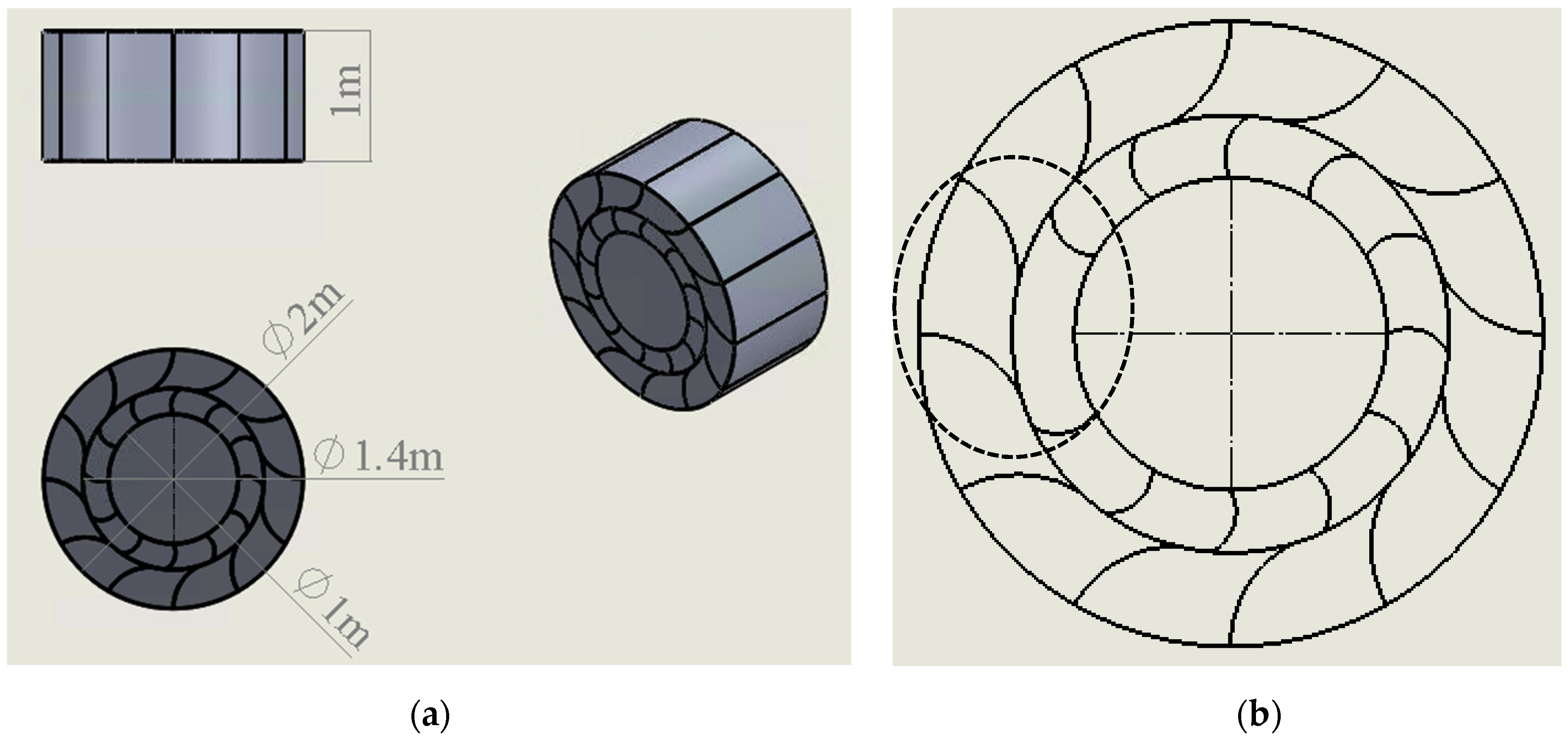
2.1. Geometry of the Vertical Axis Wind Turbine

The VAWT used in the present study consists of 12 rotor and 12 stator blades, as shown in Figure 1a. This VAWT has been used in many previous analytical, experimental, and numerical studies by the author [17,21,22,23,24] and colleagues [11,12,13,14,15,16,18,19,20]. The core, rotor, and stator outer diameters of this VAWT are 1 m, 1.4 m, and 2 m, respectively, while the height (h) is 1 m. For the damaged VAWT, we have removed one of the rotor blades (see Figure 1b). Note that the geometric centres of the VAWT models throughout this study are at (0,0,0).

The dimensions of the flow domain were obtained after carrying out extensive initial numerical assessments, ensuring that the flow fields of the VAWT models (both healthy and damaged) do not interact with the boundary conditions, especially at the inlet, top/bottom, and sides of the flow domain. Based, on these results, the specified length, width and height of the flow domain are 15 m, 3 m, and 6 m, respectively, as shown in Figure 2a. The flow domain was divided into two sections, i.e., the inner and outer sections, in order to control the mesh quality and, thus, for accurately capturing the dynamic behaviour of the wake. Based on initial assessments, it was revealed that the wake region of a VAWT extends 4D downstream (D being the dimeter of the stator). Thus, the inner section of the domain is rectangular in shape with a cylindrical head, where the diameter of the cylindrical head is 2.5 m and the total length of the section is 10.25 m. The complete flow domain, including the healthy VAWT model, is shown in Figure 2b.

2.2. Meshing of the Flow Domain

The meshing of the flow domain was carried out in three different parts, corresponding to the geometry of the flow domain. The VAWT has been spatially discretized using 15-mm hexahedral elements, with a higher concentration on the interface between the rotor and the stator regions, as shown in Figure 3a. As in the case of any turbomachine, hexahedral elements are preferred in the impeller zones [25,26]. The inner domain section was spatially discretized with hexahedral dominant mesh elements having a size of 30 mm, as shown in Figure 3b. The outer section of the domain was meshed with 100 mm tetrahedral elements.

It is well-established that a mesh suitable for the Reynolds-Averaged Navier–Stokes (RANS) simulation is not suitable for Scale-Resolving Simulations (SRS), such as LES [27]. The aforementioned element sizes were chosen after a number of initial simulations in order to find the optimal mesh size, where optimal in this context means the balance between the computational cost and the percentage of Turbulent Kinetic Energy (k) captured within the flow domain (especially in the VAWT and the wake region). For this purpose, we defined the following Custom Field Function (CFF):

$${\mathrm{a}}_{\mathrm{r}}=\frac{\sqrt{{\mathrm{A}}_{\mathrm{f}}}}{2\mathrm{y}}$$

(1)

In Equation (1), a_r is the ratio of cell-base length scale to the cell height and is used to analyse the mesh quality in the near-wall regions, which, in the current scenario, are the rotor and stator blades. A_f is the face area of the mesh elements (in m²) and y is the cell-wall distance (in m). a_r values of <10 are acceptable for LES simulations. Figure 4a depicts the spatial distribution of a_r on plane Z = 0. It can be seen that a_r values in the near-wall regions are higher than anywhere else in the flow domain (as expected), with a maximum value of 4.6. Thus, it can be safely concluded that the near-wall regions have been spatially discretized reasonably well.

In order to quantify the appropriateness of the mesh quality used in the rest of the flow domain, we defined another CFF:

$$\frac{{\mathrm{l}}_{\mathrm{o}}}{∆}=\frac{{\mathrm{k}}^{1.5}}{\mathsf{\epsilon }\sqrt[3]{\mathrm{V}}}$$

(2)

In Equation (2), lo/Δ is the ratio of integral length scale to the number of elements and is used to analyse cumulative k against the length-scale of eddies based on Kolmogorov’s energy spectrum. ε is the dissipation rate of k (in m²/s³) and V is the cell volume (in m³). lo/Δ ≥ 1.25 ensures that ≥50% of k is resolved, ≥4.8 ensures ≥80% resolution, and ≥12.5 ensures ≥90% resolution. Figure 4b depicts the spatial distribution of lo/Δ on plane Z = 0 for lo/Δ ≥ 1.25. The regions that are not covered by contour plots represent k resolution of ≥50%. It can be observed that k has been resolved reasonably well in the flow domain. For reference, we also present the spatial distributions of lo/Δ ≥4.8 and ≥12.5 in Figure 4c,d. It can be observed that most of the wake region has a k resolution of ≥80%. Thus, it can be concluded that the mesh quality in the flow domain is reasonably accurate to carry out LES.

2.3. Boundary Conditions and Fluid Properties

The inlet/upstream boundary of the flow domain was modelled as velocity inlet (U). The average wind speed in the UK (8.2 knot or 4.2 m/s) was prescribed to the VAWT models. The outlet/downstream face of the flow domain was modelled as a pressure outlet boundary, with 0 Pa,g pressure, assuming that the outlet boundary is far away from the VAWT and there are no interactions between the two (this will become evident later in the results section). The top/bottom and the side walls of the domain have been modelled as walls, translating in +X direction at 4.2 m/s—the same as the inlet wind velocity—in order to avoid build-up of shear layers. The stator blades remain fixed, i.e., stationary walls with no-slip boundary condition. The numerical simulations were carried out assuming isothermal conditions, with air having a density (ρ) and dynamic viscosity (μ) of 1.225 kg/m³ and 1.789 × 10⁻⁵ kg/m/s, respectively.

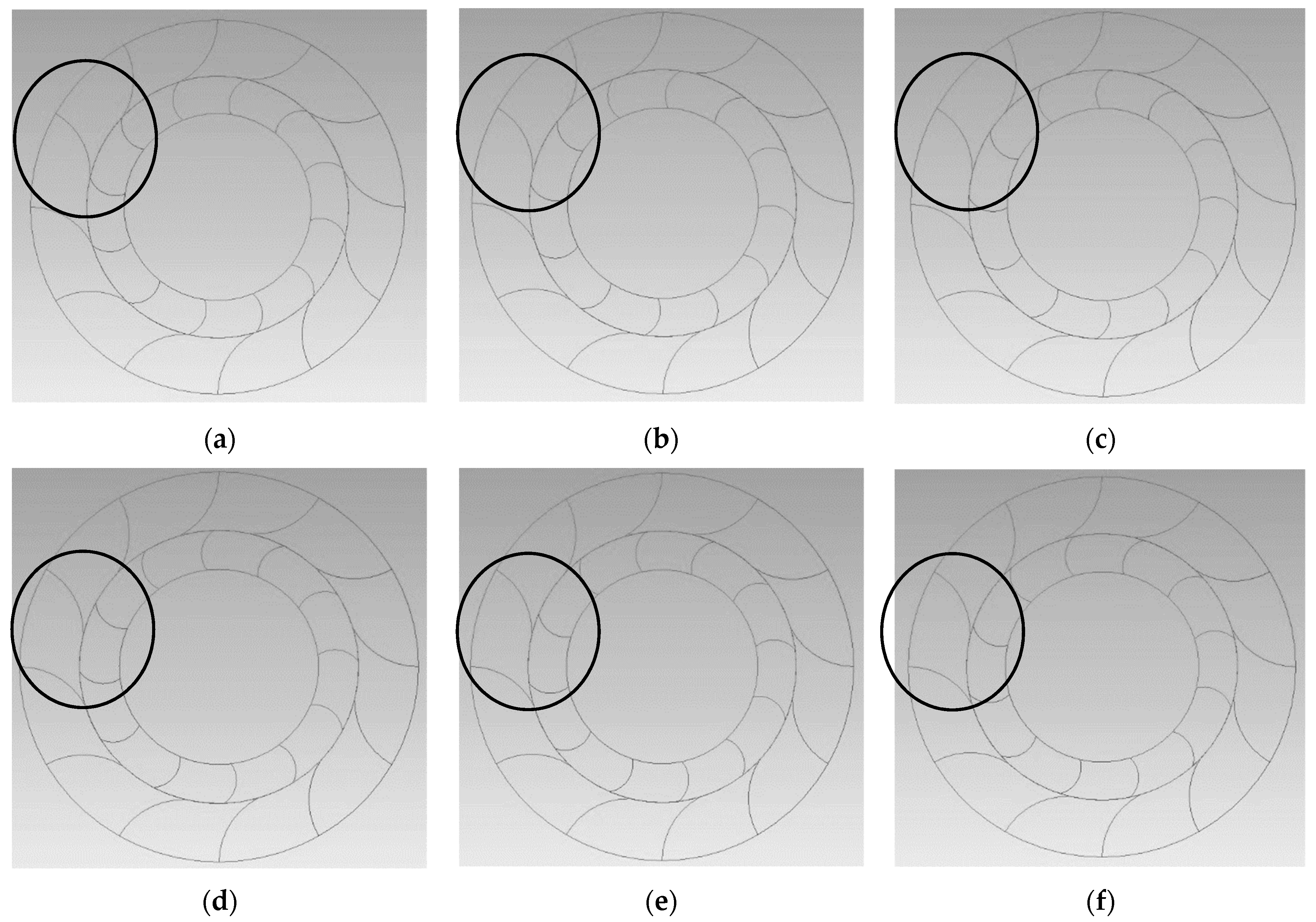
2.4. Rotation of the Vertical Axis Wind Turbine

As discussed earlier, the VAWT considered in the present study is a Savonius VAWT. Studies show that the Savonius VAWTs have a peak Power Coefficient (C_p) at a Tip Speed Ratio (λ) of about 0.5 [28]. C_p and λ are defined here as

$${\mathrm{C}}_{\mathrm{p}}=\frac{\mathrm{P}}{\frac{1}{2}\mathsf{\rho }\mathrm{A}{\mathrm{U}}^3}$$

(3)

and

$$\mathsf{\lambda }=\frac{\mathsf{\omega }\mathrm{R}}{\mathrm{U}}$$

(4)

where

• P is the power generated by the VAWT; P = ωT, where ω is the rotational speed (in rad/s) and T is the torque (in Nm) generated by the rotor.
• A is the swept area of the VAWT (in m²); A = Dh, where D is the rotor’s outer diameter (=1.4 m) and h is the height of the VAWT (=1 m).
• R is the rotor radius (in m); R = D/2 = 0.7 m.

Based on λ = 0.5, R = 0.7 m, and U = 4.2 m/s, using Equation (4), we obtain ω = 3 rad/s or ~29 rpm, which was specified as the rotational speed of the rotor.

2.5. Turbulence Modelling

Large Eddy Simulation (LES) was employed in the present study to model air turbulence, in which the large-scale turbulent motion is resolved, while the small-scale turbulent motion is modelled. For large-scale eddies, filtered Navier–Stokes equations have been used, while for small-scale eddies, subgrid-scale (SGS) modelling was employed. LES applies spatial averaging, rather than temporal averaging, to the momentum transport equation; thus, LES solutions are time-dependent, which is more beneficial for the case of turbomachinery, such as VAWTs, because the effects of rotor blades rotation can be captured more accurately w.r.t. time. It is noteworthy here that the entire turbulence spectrum can be resolved using Direct Numerical Simulations (DNS); however, it is not feasible for practical engineering applications involving high Reynolds number flows due to its exorbitant computational cost (~Re_t³) [29,30].

The filtered Navier–Stokes (NS) equations can be written as follows:

$$\frac{\partial \mathsf{\rho }}{\partial \mathrm{t}}+\frac{\partial }{\partial {\mathrm{x}}_{\mathrm{i}}}\left({\mathsf{\rho }\overline{\mathrm{u}}}_{\mathrm{i}}\right)=0$$

(5)

$$\frac{\partial }{\partial \mathrm{t}}\left({\mathsf{\rho }\overline{\mathrm{u}}}_{\mathrm{i}}\right)+\frac{\partial }{\partial {\mathrm{x}}_{\mathrm{j}}}\left({\mathsf{\rho }\overline{\mathrm{u}}}_{\mathrm{i}}{\overline{\mathrm{u}}}_{\mathrm{j}}\right)=\frac{\partial }{\partial {\mathrm{x}}_{\mathrm{j}}}\left({\mathsf{\sigma }}_{\mathrm{ij}}\right)-\frac{\partial \overline{\mathrm{p}}}{\partial {\mathrm{x}}_{\mathrm{i}}}-\frac{\partial {\mathsf{\tau }}_{\mathrm{ij}}}{\partial {\mathrm{x}}_{\mathrm{j}}}$$

(6)

where the stress tensor due to molecular viscosity (σ_ij) can be defined as follows:

$${\mathsf{\sigma }}_{\mathrm{ij}}=\left[\mathsf{\mu }\left(\frac{\partial {\overline{\mathrm{u}}}_{\mathrm{i}}}{\partial {\mathrm{x}}_{\mathrm{j}}}+\frac{\partial {\overline{\mathrm{u}}}_{\mathrm{j}}}{\partial {\mathrm{x}}_{\mathrm{i}}}\right)\right]-\frac{2}{3}\mathsf{\mu }\frac{\partial {\overline{\mathrm{u}}}_{\mathrm{l}}}{\partial {\mathrm{x}}_{\mathrm{l}}}{\mathsf{\delta }}_{\mathrm{ij}}$$

(7)

The SGS stress (τ_ij) requires further modelling, employing Boussinesq hypothesis, as follows:

$${\mathsf{\tau }}_{\mathrm{ij}}=\mathsf{\rho }\overline{{\mathrm{u}}_{\mathrm{i}}{\mathrm{u}}_{\mathrm{j}}}-{\mathsf{\rho }\overline{\mathrm{u}}}_{\mathrm{i}}{\overline{\mathrm{u}}}_{\mathrm{j}}$$

(8)

Here, μ_t is the turbulent viscosity at SGS (also called eddy viscosity), which needs to be modelled. It has been discussed earlier that SGS eddies are assumed to be isotropic, essentially meaning that SGS stresses (τ_kk) are not modelled; instead, they are added to the filtered static pressure term. The rate of strain tensor δ_ij can be defined as

$${\overline{\mathrm{S}}}_{\mathrm{ij}}\equiv \frac{1}{2}\left(\frac{\partial {\overline{\mathrm{u}}}_{\mathrm{i}}}{\partial {\mathrm{x}}_{\mathrm{j}}}+\frac{\partial {\overline{\mathrm{u}}}_{\mathrm{j}}}{\partial {\mathrm{x}}_{\mathrm{i}}}\right)$$

(9)

For modelling μ_t, we have used the Wall Adapting Local Eddy Viscosity (WALE) model, where μ_t can be defined as

$${\mathsf{\mu }}_{\mathrm{t}}={\mathsf{\rho }\mathrm{L}}_{\mathrm{s}}{}^2\frac{{\left({\mathrm{S}}_{\mathrm{ij}}{}^{\mathrm{d}}{\mathrm{S}}_{\mathrm{ij}}{}^{\mathrm{d}}\right)}^{\frac{3}{2}}}{{\left({\overline{\mathrm{S}}}_{\mathrm{ij}}{\overline{\mathrm{S}}}_{\mathrm{ij}}\right)}^{\frac{5}{2}}+{\left({\mathrm{S}}_{\mathrm{ij}}{}^{\mathrm{d}}{\mathrm{S}}_{\mathrm{ij}}{}^{\mathrm{d}}\right)}^{\frac{5}{4}}}$$

(10)

where L_s is the subgrid-scale mixing length, which is computed as

$${\mathrm{L}}_{\mathrm{s}}=\min \left(\mathsf{\kappa }\mathrm{d},{\mathrm{C}}_{\mathrm{w}}{\mathrm{V}}^{\frac{1}{3}}\right)$$

(11)

Here, κ is the von Karman constant, d is the distance to the closest wall, C_w is a constant having a value of 0.325, and V is the cell volume.

$${\mathrm{S}}_{\mathrm{ij}}{}^{\mathrm{d}}=\frac{1}{2}\left({\overline{\mathrm{g}}}_{\mathrm{ij}}^2+{\overline{\mathrm{g}}}_{\mathrm{ji}}^2\right)-\frac{1}{3}{\mathsf{\delta }}_{\mathrm{ij}}$$

(12)

$${\overline{\mathrm{g}}}_{\mathrm{ij}}=\frac{\partial {\overline{\mathrm{u}}}_{\mathrm{i}}}{\partial {\mathrm{x}}_{\mathrm{j}}}$$

(13)

2.6. Temporal Discretisation

As with spatial discretization, temporal discretization is also crucial for the accuracy of time-dependent numerical solutions; however, the computational cost also needs to be reasonable. Thus, we defined a Custom Field Function (CFF) for the determination of appropriate time step, for time advancing solutions, as follows:

$$∆\mathrm{t}=\frac{{\mathrm{V}}^{\frac{1}{3}}}{\left|\mathrm{U}\right|}$$

(14)

where V is the cell volume (in m³) and |U| is the local flow velocity magnitude (in m/s). The lower limit of Δt, which can capture all of the flow domain, is recommended for LES; however, higher Δt can be used. Figure 5 depicts the spatial distribution of Δt within the flow domain. In Figure 5a, the lower limit is set to 0.005747 s, which is equivalent to 1° rotation of the rotor, while in Figure 5b, the lower limit is set to 0.5° rotation. It can be seen that most of the flow domain (except upstream stator and rotor zones) can be reasonably captured using a Δt of 1° per time step. The temporal resolution can be further improved by considering 0.5° per time step. Obviously, there is trade-off between better temporal resolution and computational resources available/required; we have considered 1° rotation of the rotor blades per time step in the present study.

3. Results and Discussions

After running the precursor RANS simulations, we carried out Large Eddy Simulations (LES) on the healthy and damaged (one rotor blade missing) VAWT models, and the results are presented in this section. The LES simulations were run long enough in order to obtain a statistically steady solution (a few revolutions). Thereafter, we have recorded numerical data for processing and analysis. In this section, we will start our discussion with a brief analysis of the torque signals from both the VAWT models and quantify the differences between the two. Then, we will analyse the time-dependent pressure, velocity, and vorticity fields of healthy and damaged VAWTs. Afterwards, we present the Proper Orthogonal Decomposition (POD) methodology employed, followed by an extensive comparative analysis of the POD modes based on pressure, velocity, and vorticity fields.

3.1. Torque Output Comparison between Healthy and Damaged VAWTs

Torque (T) generated by the rotor blades of the VAWT can be computed as

$$\mathrm{T}=\frac{1}{2}{\mathrm{C}}_{\mathrm{T}}\mathrm{A}\mathrm{R}\mathsf{\rho }{\mathrm{U}}^2$$

(15)

where C_T is the torque coefficient of the VAWT, A is the swept area of the VAWT (in m²), R is the rotor radius (in m), ρ is the density of air (in kg/m³), and U is the incident flow velocity on the blades (in m/s). Torque signals for one full revolution of healthy and damaged VAWTs have been plotted in Figure 6. It can be seen that (as in many published studies as well) the amplitude of torque signal from the damaged VAWT seems to be higher than the healthy VAWT. The −ve peaks in case of damaged VAWTs depict significantly lower torque values compared with healthy VAWT; thus, it is expected that the average torque output from the damaged VAWT will be lower than the healthy VAWT. In order to ensure this, basic statistical analyses were performed on both the torque signals. The results are summarized in

Table 1. Torque characteristics of healthy and damaged VAWTs.

Torque Characteristics	Healthy VAWT	Damaged VAWT	Difference w.r.t. Healthy VAWT
	(Nm)	(Nm)	(%)
Average	5.8	5.6	−2.52
Maximum	6.7	7.2	+7.46
Minimum	5.0	4.4	−12.39
Amplitude	1.7	2.8	+66.52

. As expected, the average torque output from the damaged VAWT is 2.52% lower than the healthy VAWT, while its amplitude is 66.52% higher. This indicates that the damaged VAWT experiences significantly higher wind loads, which can have a considerable impact on its structural health. In published literature [8,9,10], researchers have extensively used digital signal processing techniques to find out the dominant frequencies in the torque signals and have attempted to link them to the damage the VAWT has experienced.

In order to validate the numerical results obtained in this study, the power coefficient (Cp) of the healthy VAWT was compared against the experimental data of Gareth [31] for the same VAWT. Using the well-known relationship between the power and torque outputs of a VAWT (P = ωT), average power of the healthy VAWT was computed to be 17.3 W. Using Equation (3), Cp of the healthy VAWT has been computed to be 0.19, while Gareth [31] obtained a Cp of 0.188 for the same VAWT at λ = 0.5. Thus, there is a close match between the numerically predicted and experimentally recorded Cp values of the healthy VAWT model considered in the present study.

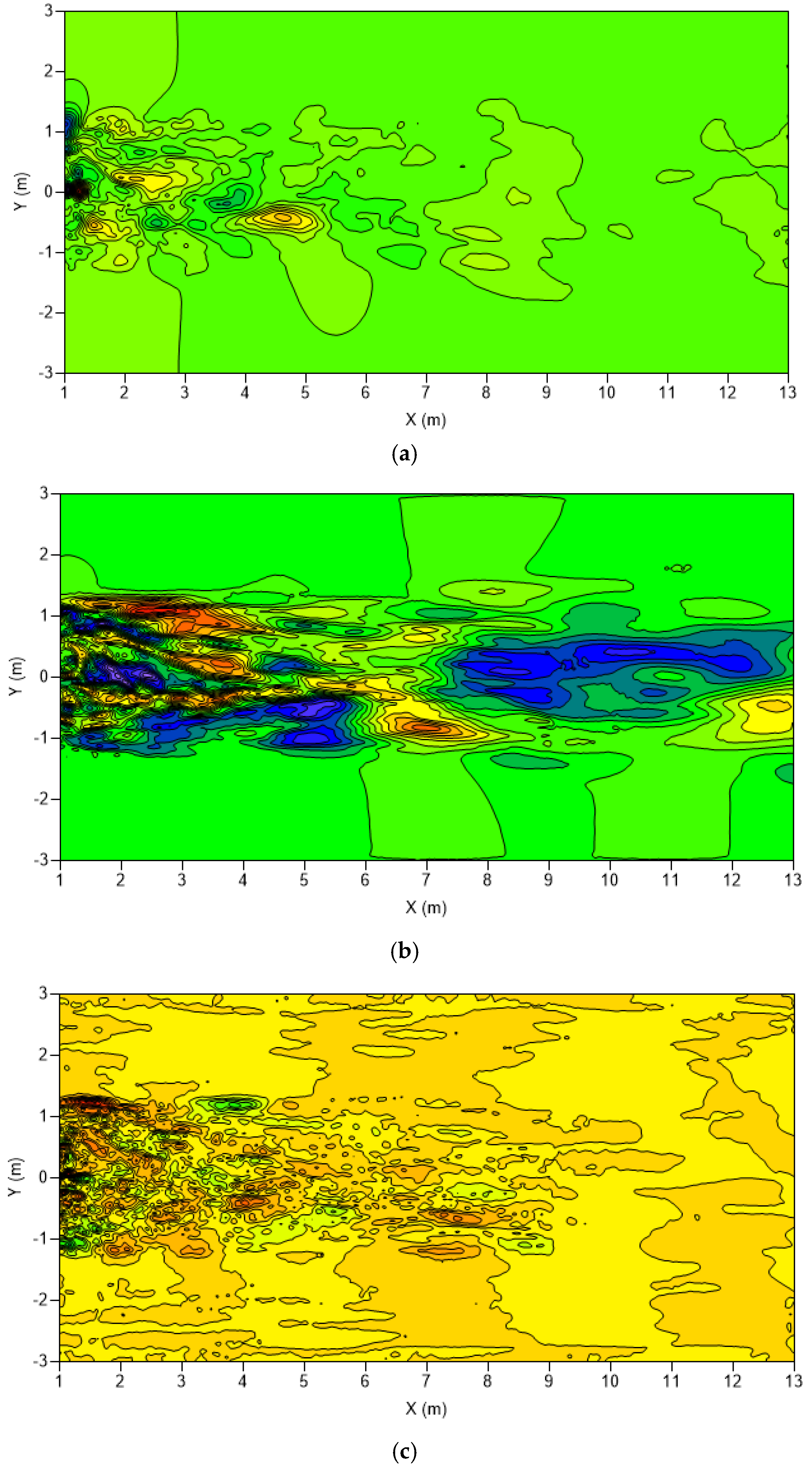
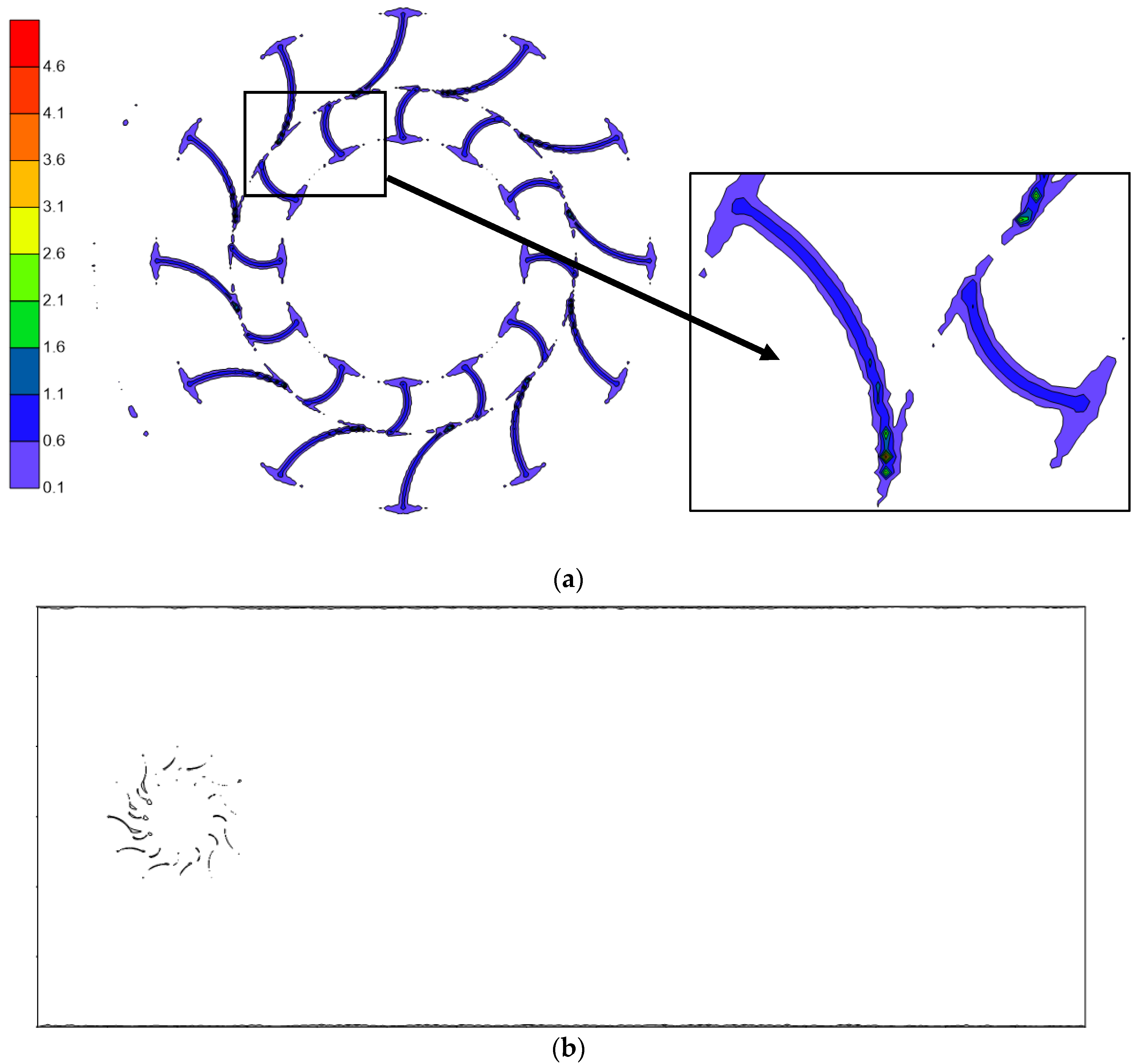
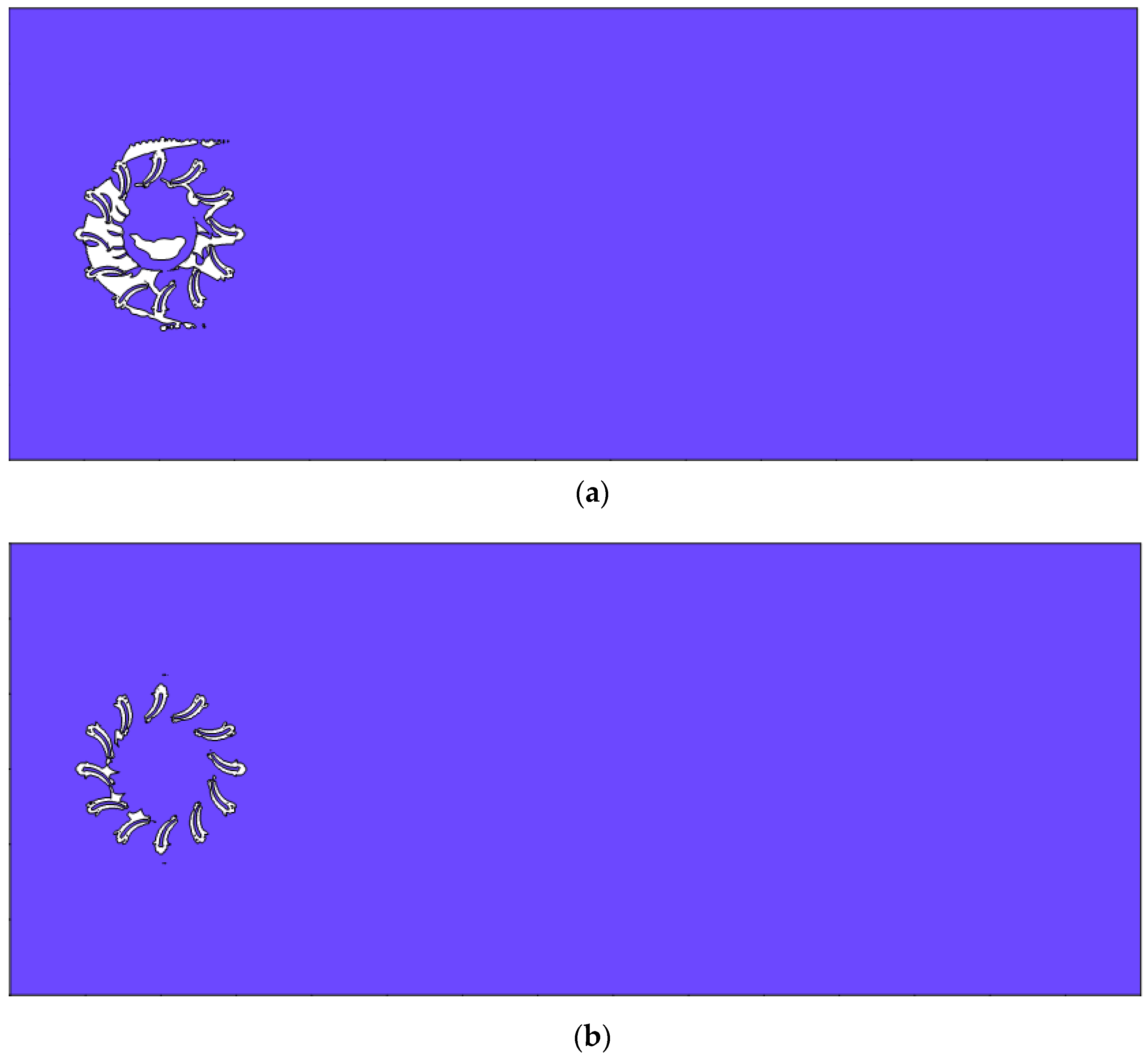
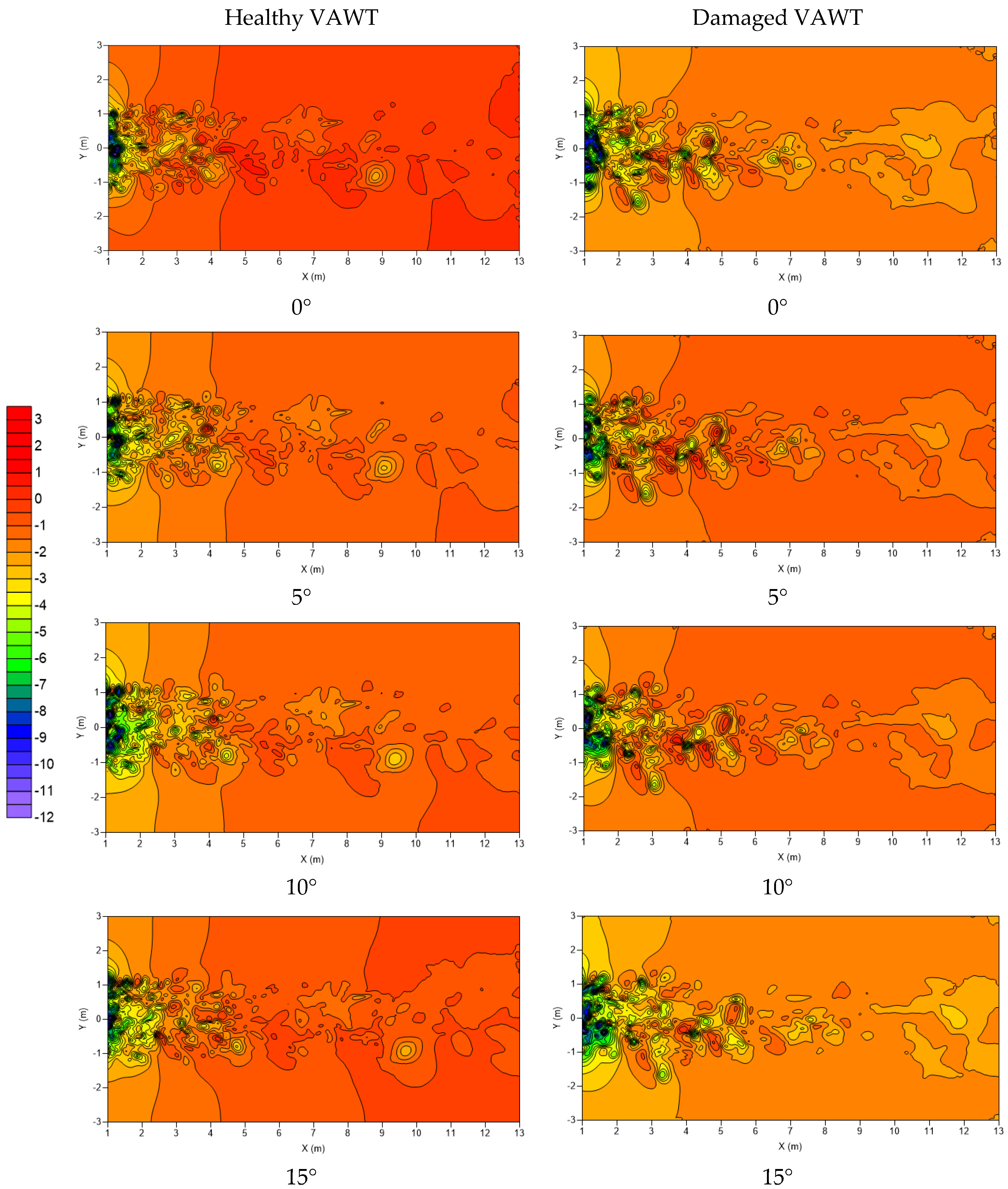
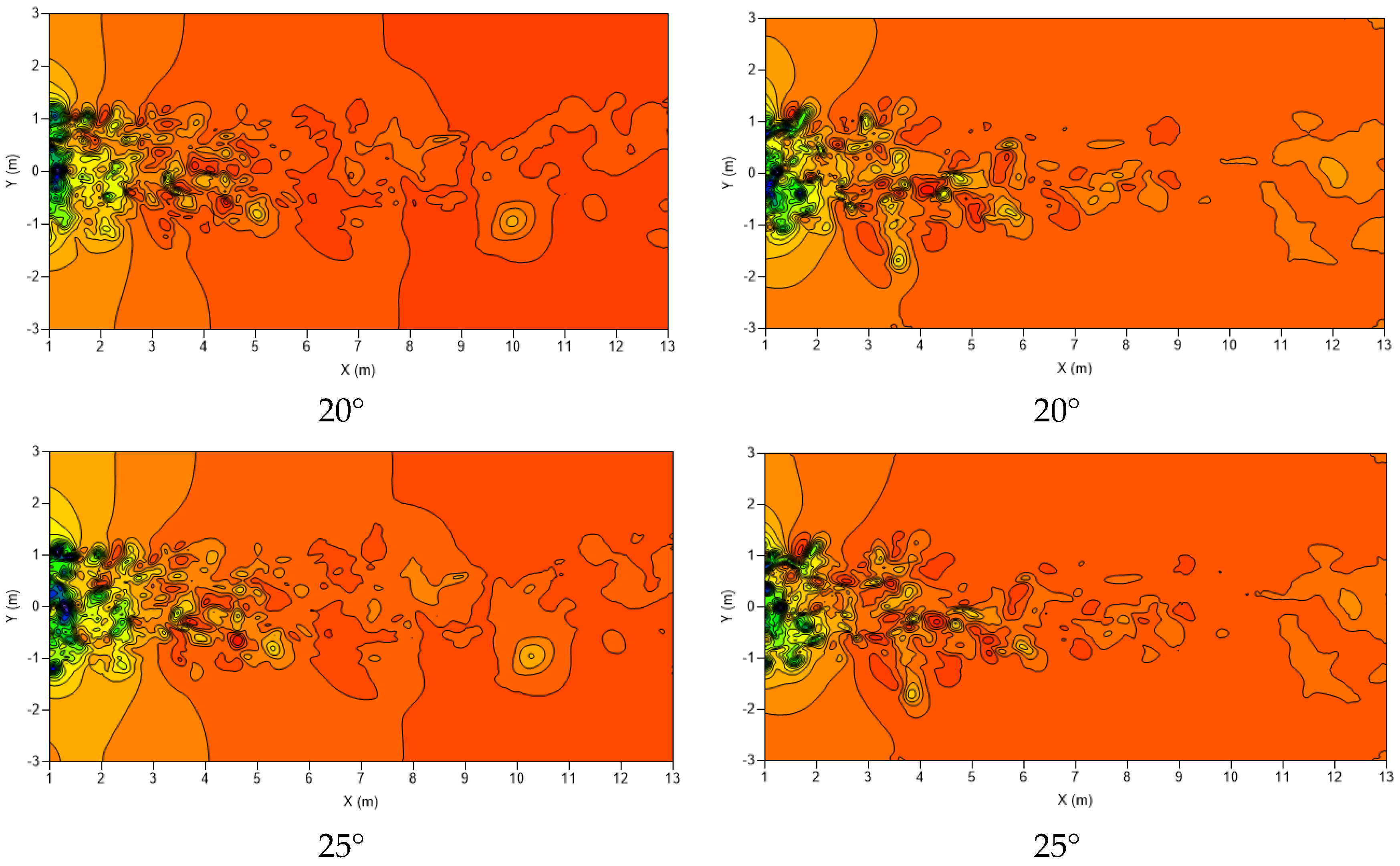
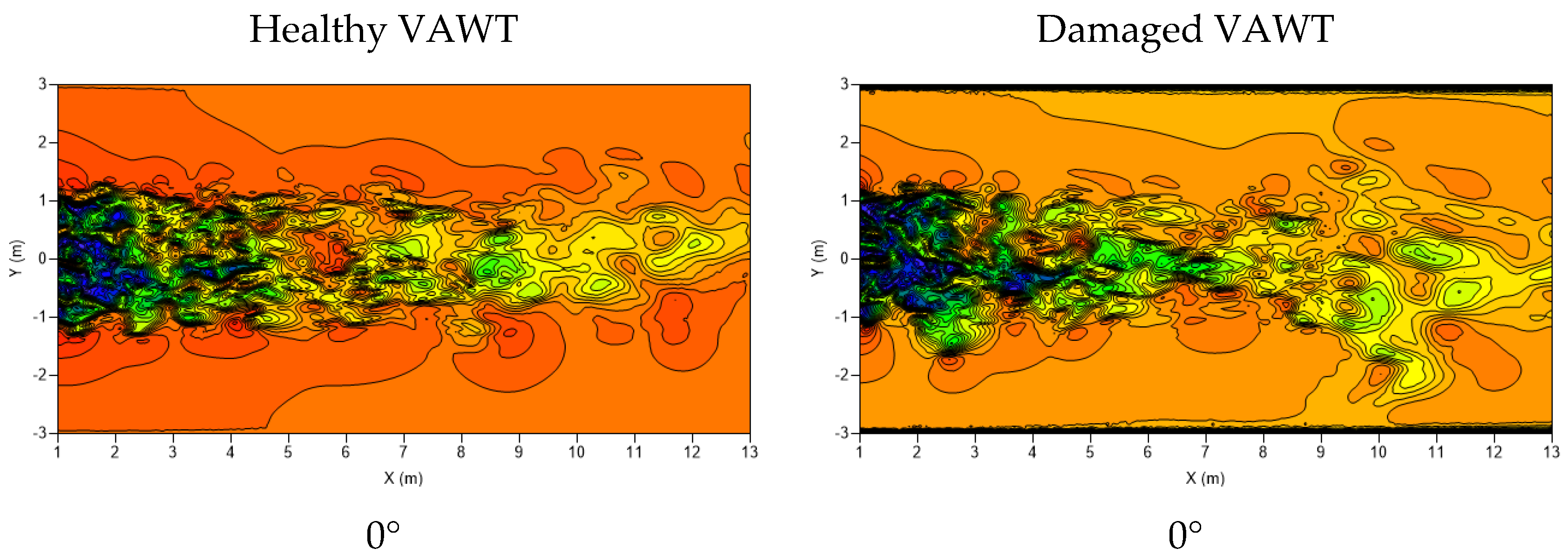
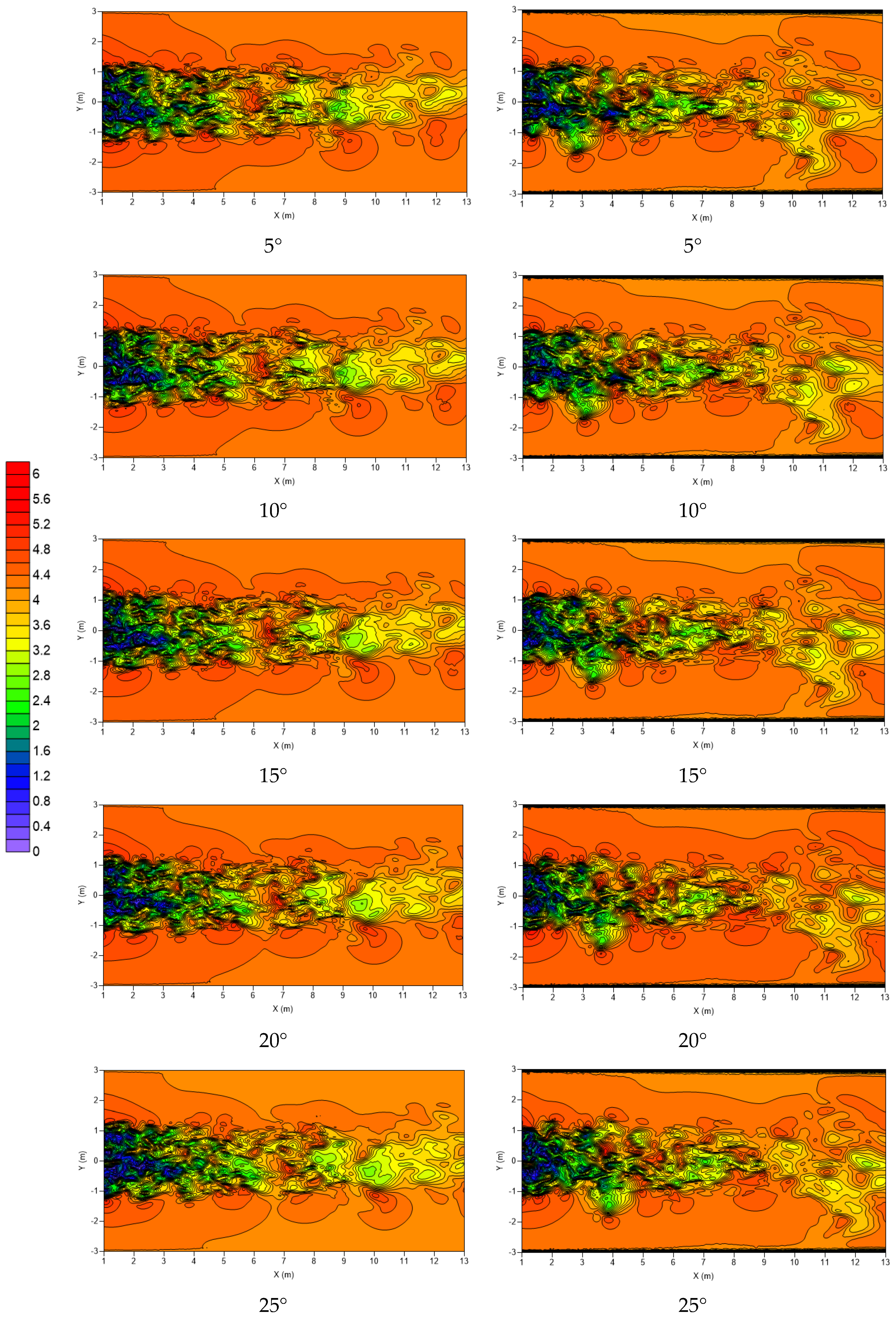
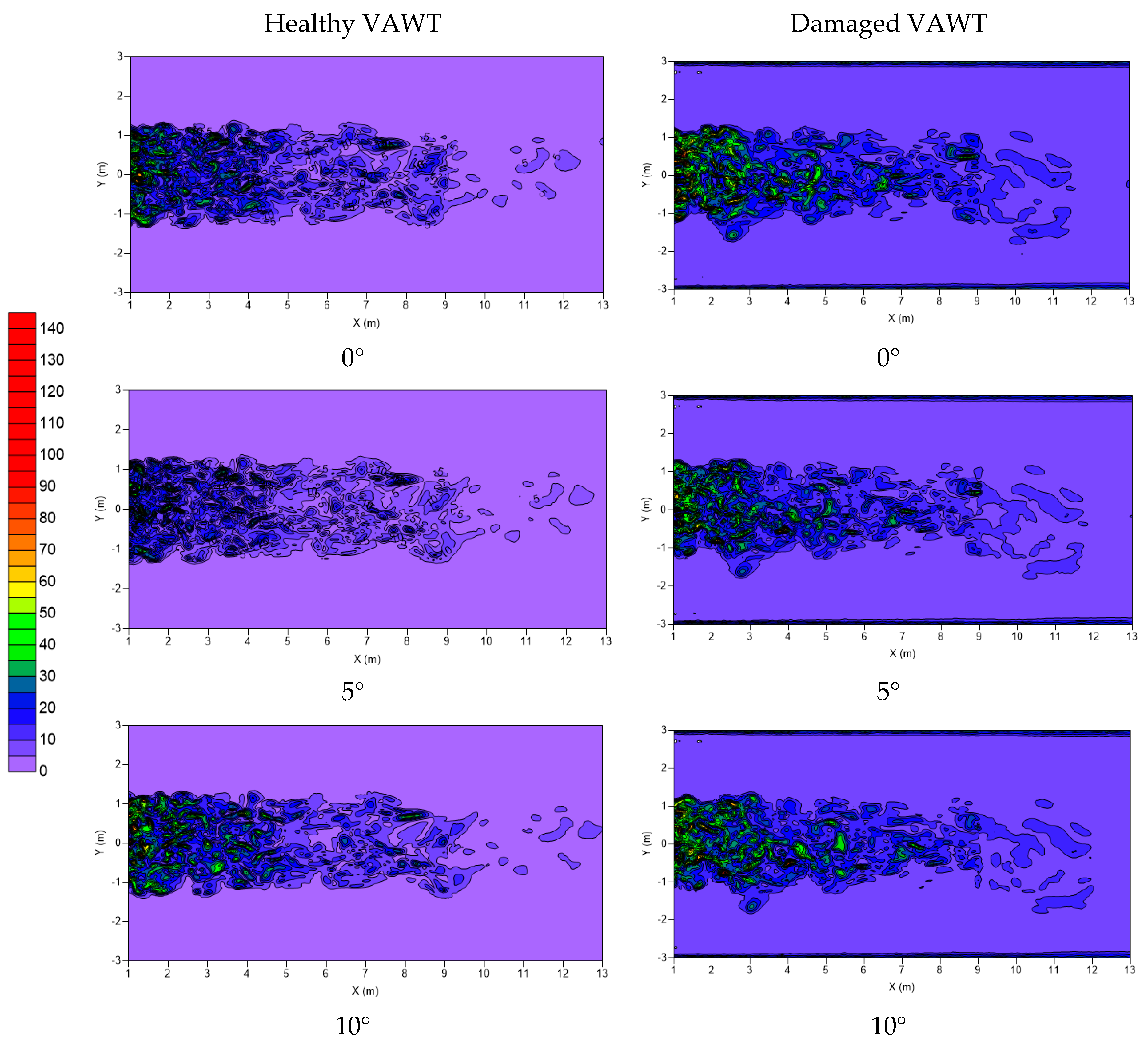
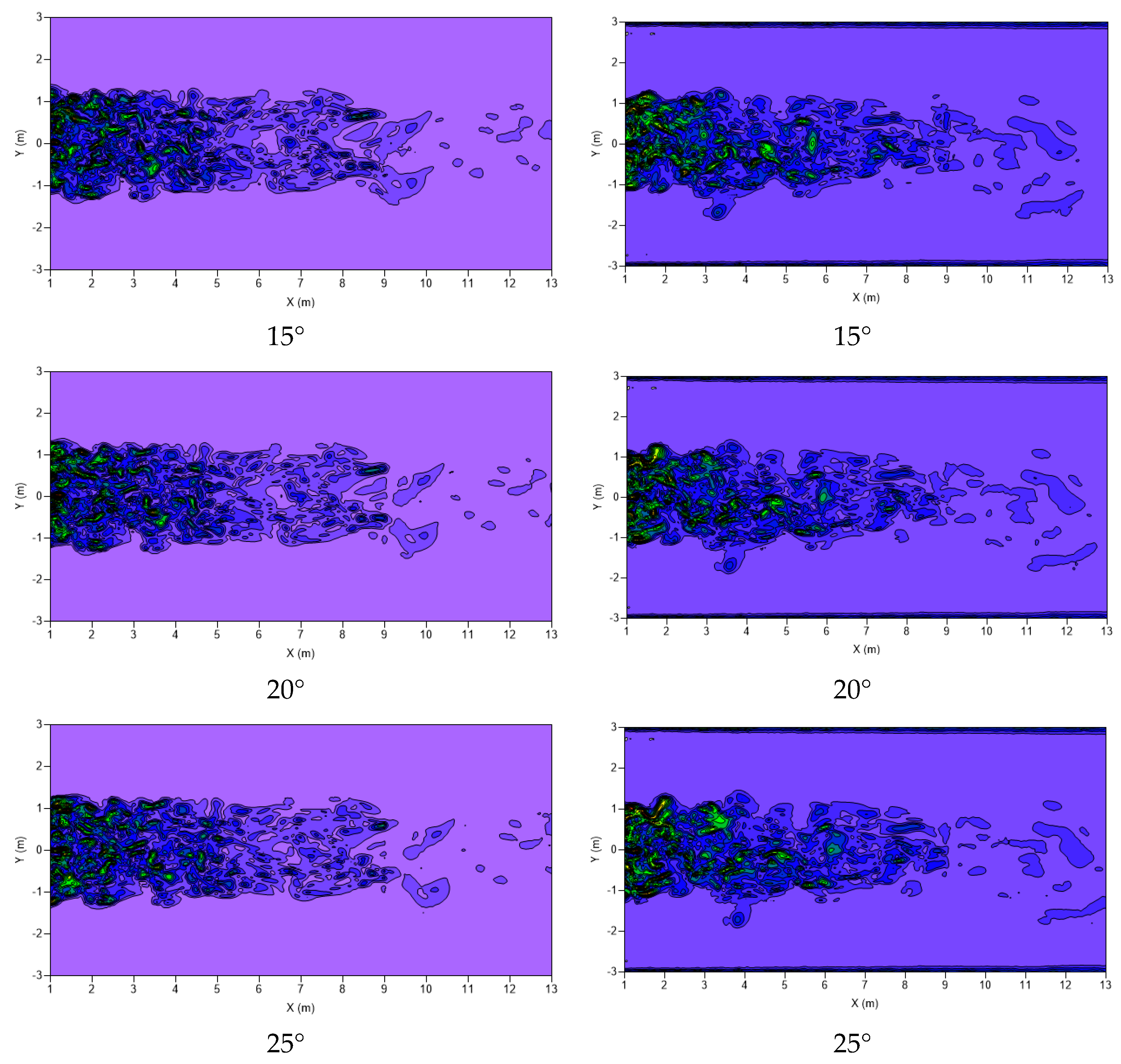
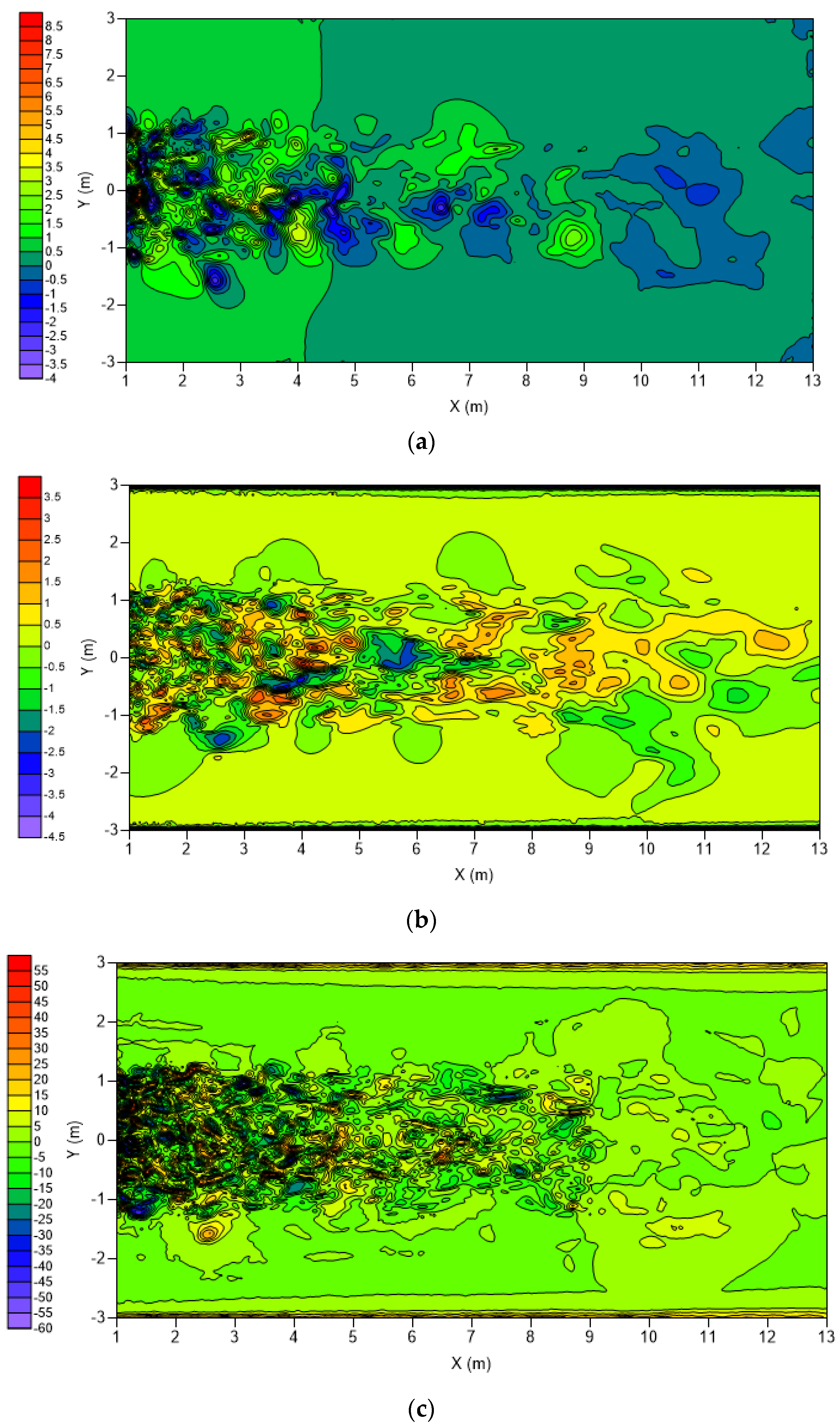
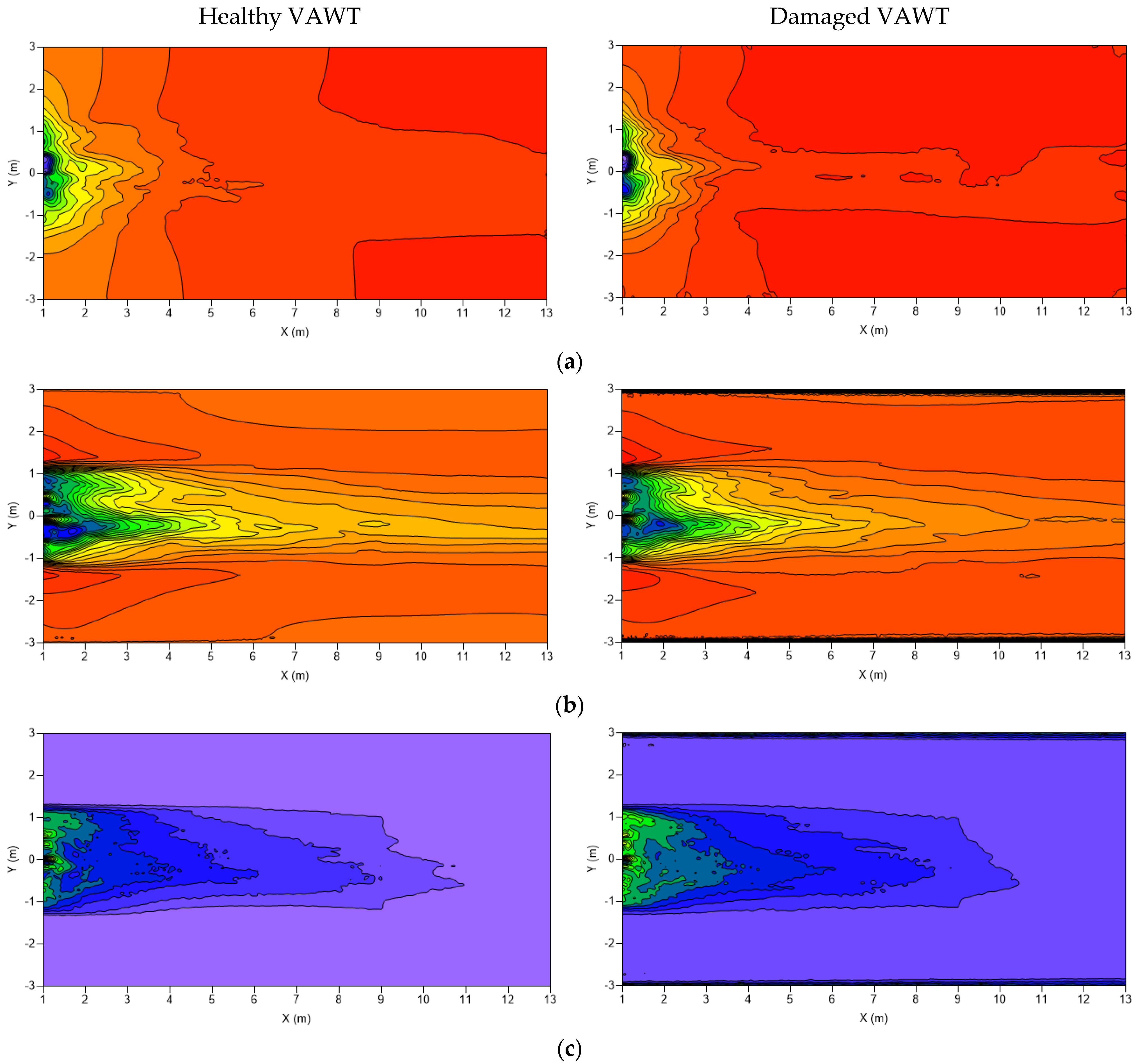
3.2. Flow Field Analysis of Healthy and Damaged VAWTs

In this section, we will analyse the pressure, velocity, and vorticity fields of both healthy and damaged VAWTs, with a view to identify (and compare) the differences between them. For this purpose, we will use the flow field data on plane Z = 0 at six different rotor blades’ positions, from 0° to 25° with equal intervals of 5°. The reason for choosing these blade positions is that they cover the complete journey of a rotor blade from being in-line with a stator blade to the time when it reaches the next stator blade. This is more evident in Figure 7. It is noteworthy that although rotor torque signals in Figure 6 are not exactly the same during a revolution of the VAWT, they are largely within a certain range; thus, we will be analysing the said blade positions only.

Figure 8 depicts the spatial distribution of static pressure in the wake region of the healthy and damaged VAWTs. As our focus in this study is to better understand the dynamic behaviour of wakes, our analysis will be limited to the wake regions only. It is evident in Figure 8 that the wake regions of both the VAWTs contain very complex flow features. The presence and propagation of coherent structures can be clearly observed. Coherent structures, as defined by Berkooz et al. [32], are organized spatial features that appear in shear flows and have a characteristic temporal life cycle. Coherent features were first discovered by Liu [33] and are considered inherent to fully turbulent flows. It can be seen that coherent flow structures feed into the wake region downstream of both the VAWTs. These structures break apart from the main wake flow to form localized low-pressure pockets, dissipating energy as they propagate further downstream. In case of damaged VAWT, we make two observations here:

• Pressure in the wake region is slightly higher, on average, than the pressure in the wake region of the healthy VAWT;
• The breakup of coherent structures is more complex/nonuniform and these structures are still present further downstream than the healthy VAWT.

The aforementioned observations are, however, qualitative in nature, and further investigated are needed as the pressure field comparison is lacking obvious major differences between the two VAWT models.

Figure 9 depicts the spatial distribution of flow velocity magnitude in the wake regions of healthy and damaged VAWTs. The coherent structures are again obvious and are spread more nonuniformly in case of damaged VAWT. As noticed in case of pressure field, there seems to be some minor differences between the two wake regions; the flow velocity, on average, seems slightly lower in the wake region of the damaged VAWT as compared with the healthy VAWT. It is clear that using standard Computational Fluid Dynamics (CFD)-based techniques, it is extremely difficult to quantify the differences between the two wake regions shown, as also stated by Sirovich [34]. The reason for this difficulty in analysing (and comparing) the flow fields is that CFD computes the resultant (combined) flow variables, which is obviously dominated by the main air flow (in +X direction) for VAWTs. As the resultant flow field comprises hundreds of individual components, for accurate quantification of the differences between healthy and damaged VAWTs, it is essential to break the flow fields down into their individual components.

The vorticity distribution shown in Figure 10 provide similar insights about the wake regions of healthy and damaged VAWT models, with some visual differences between the two. The vortices in case of the damaged VAWT seems to be stronger than the healthy VAWT (based on the scale) and extend further downstream in the wake. As previously, without breaking the resultant flow fields into individual components, accurate quantification of the wake dynamics is very difficult. This is of particular interest in the present context for the recognition of distinct patterns in the wake flow fields. It is envisaged that this study will provide a functional basis for the development of better flow control mechanisms and machine learning algorithms. For reader’s interest, we provide the time-averaged spatial distribution of pressure, velocity, and vorticity fields of both the healthy and damaged VAWTs in Appendix A.

Before moving towards breakdown of the flow fields into their individual components, another statistical technique that has recently been used for flow field comparisons in some studies [35,36,37,38] is discussed here. The difference between the flow fields of healthy and damaged VAWTs, for the same flow parameter, can be computed as

$${\mathsf{\phi }}_{\mathrm{difference}}={\mathsf{\phi }}_{\mathrm{damaged}}-{\mathsf{\phi }}_{\mathrm{healthy}}$$

(16)

Figure 11 depicts the spatial distribution of φ_difference for the pressure, velocity, and vorticity fields. It can be seen in Figure 11a that the local pressure differences range from −4 Pa,g to +8.5 Pa,g. The distribution of positive and negative pressure zones across Y = 0 m, which is an inherent characteristic of VAWTs, indicates stronger vortices shed by the damaged VAWT compared with the healthy VAWT. Figure 11b,c also depict similar trends, i.e., higher flow velocity and vortex shedding in damaged VAWT. The issue here is that the differences in flow variables are still based on resultant values and, thus, are resultant in nature themselves.

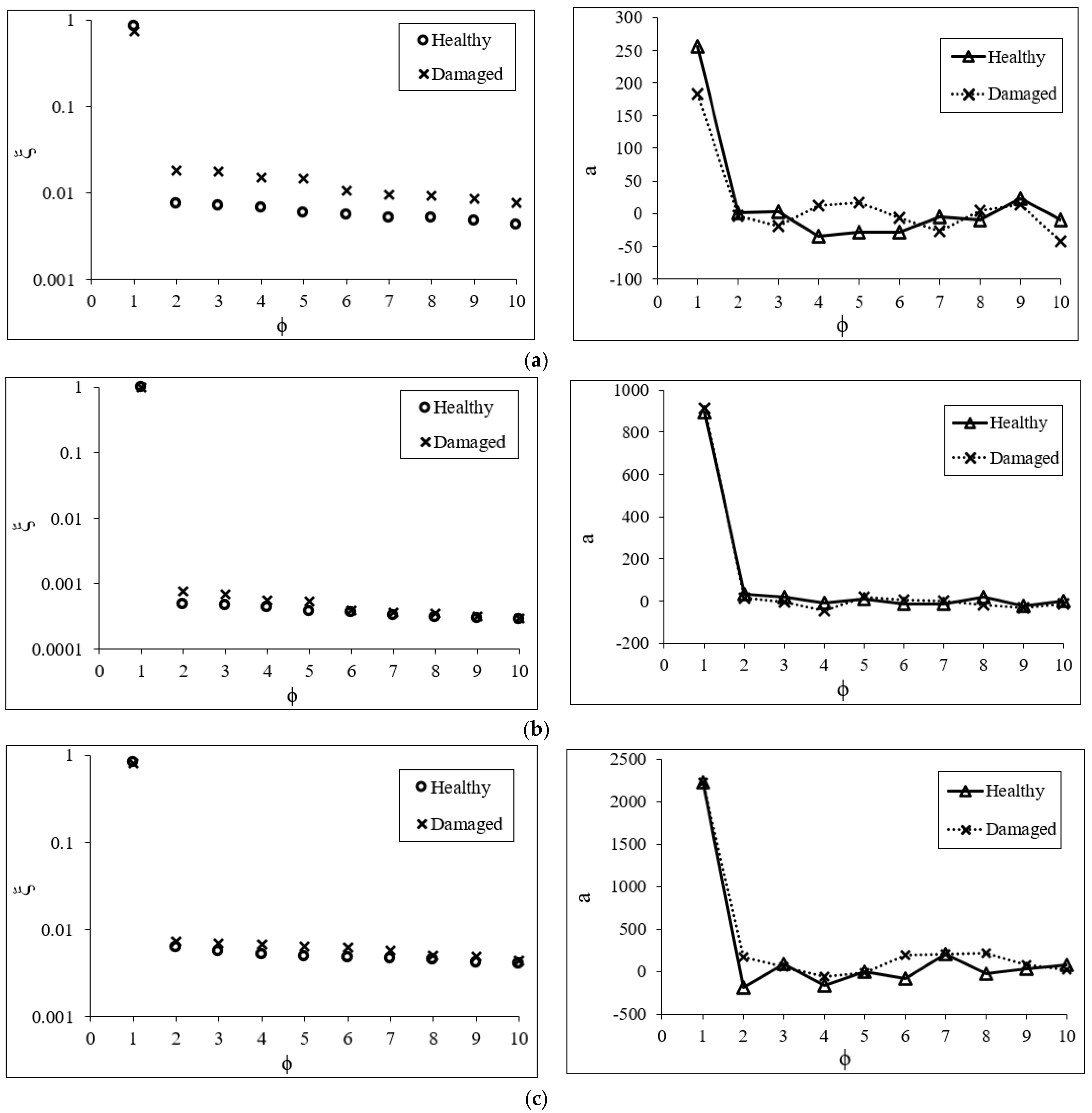
3.3. Proper Orthogonal Decomposition (POD)

It is well-established (through the results presented in Section 3.1 and from the literature review) that a missing rotor blade has a significant effect on the torque generating capability of the VAWT. Let us first break this torque degradation phenomena/event down into different stages. In stage 1, the VAWT loses a rotor blade (catastrophic event). In stage 2, the flow field changes in order to accommodate the effects of modified geometry (flow-field re-establishment). Finally, in stage 3, the modified flow field interacts with the modified rotor blades and consequently, the blades generate torque. Most of the published studies address stage 3 (which is also very important as far as power generation from VAWTs is concerned). However, stage 3 is a consequence of stage 2, i.e., re-established flow features; thus, the root cause for torque variations lies in stage 2. Published research studies are severely limited to either space-averaged or time-averaged investigations on stage 2, which provide an overall perspective, as discussed in Section 3.2. In this study, our aim is to break the re-established flow field down into meaningful components and analyse them individually with a view to identify (and quantify) dominant patterns of coherent structures in the wake regions of healthy and damaged VAWTs. For this purpose, we use Proper Orthogonal Decomposition (POD) on the pressure, velocity, and vorticity fields.

Proper Orthogonal Decomposition (POD) is a mathematical procedure developed initially by Lumley [39] and later extended as Karhunen–Loeve expansion in pattern recognition [40,41] to decompose a time-dependent flow variable into infinite linear combinations of orthogonal, to analyse flow turbulence. There are a number of ways to achieve this, such as the Snapshot method [34], Dynamic Mode Decomposition (DMD), [42], spatiotemporal POD [30], etc., each having their own merits and demerits. In this study, we use the Snapshot method to compute the orthogonal modes of the flow fields. The reason for choosing this method is its low computational cost. For reconstruction of the original data, optimal linear basis (or modes) needs to be obtained, which reduce the order of the system however, still approximating the dynamic behaviour of the flow variable reasonably well.

Let us consider a vector field u(x,t), which can be decomposed into its deterministic spatial functions ϕ(t) and time coefficients a(t) as

$$\mathrm{u}\left(\mathrm{x},\mathrm{t}\right)={\displaystyle \sum _{\mathrm{i}=1}^{\mathrm{n}}}{\mathrm{a}}_{\mathrm{i}}\left(\mathrm{t}\right){\mathsf{\varphi }}_{\mathrm{i}}\left(\mathrm{x}\right)$$

(17)

Time-advancing snapshots of u from the LES data are recorded every Δt and arranged in matrix form. Modes of u(x,t) are computed from the ensemble of Partial Differential Equation (PDE) solutions. The inner product between the field and the mode is maximized as

$$\max \frac{{\langle \left|\mathrm{u},\mathsf{\varphi }\right|\rangle }^2}{{\Vert \mathsf{\varphi }\Vert }^2}$$

(18)

Here, the numerator is maximized for ‖ϕ‖² = 1. The modes to be computed should satisfy

$$\int \langle \mathrm{u}\left(\mathrm{x}\right)\mathrm{u}\left({\mathrm{x}}^{\prime }\right)\rangle \mathsf{\varphi }\left({\mathrm{x}}^{\prime }\right)\mathrm{d}{\mathrm{x}}^{\prime }=\mathsf{\psi }\mathsf{\varphi }\left(\mathrm{x}\right)$$

(19)

where ψ is Lagrange multiplier. The eigenfunction of Equation (18) is computed such that its kernel is the average autocorrelation function $\langle \mathrm{u}\left(\mathrm{x}\right)\mathrm{u}\left({\mathrm{x}}^{\prime }\right)\rangle =\mathrm{R}\left(\mathrm{x},{\mathrm{x}}^{\prime }\right)$. The eigenvalue problem reduces to Rϕ = ψϕ. The modes (ϕ) and corresponding eigenvalues are then computed. It is noteworthy that the eigenvalues represent the energy content (ξ) of the modes. In this study, both ξ and a (temporal coefficients), based on pressure, velocity, and vorticity data, were analysed and the corresponding POD modes (ϕ) were computed. For the validity of the POD modes, we reconstruct the flow fields and compare them in Figure 8, Figure 9 and Figure 10.

In this study, the first 10 POD modes were computed in the wake regions of healthy and damaged VAWTs. Figure 12 depicts the energy content (ξ) and the temporal coefficients (a) of these modes for the pressure, velocity, and vorticity data. It can be clearly seen that for all the flow variables considered, the first POD mode (ϕ₁) is the dominant mode. ϕ₁ in case of healthy VAWT contains 85%, 99%, and 82% of the energy for pressure, velocity, and vorticity fields, respectively. For the damaged VAWT, the corresponding ξ values for ϕ₁ are 73%, 99%, and 81%. Thus, ξ of pressure-based ϕ₁ for the damaged VAWT is 14% lower than the healthy VAWT, while the differences in ξ of velocity- and vorticity- based ϕ₁ are <1%. In case of temporal coefficients (a) as well, pressure-based ϕ₁ of damaged VAWT is 28% lower than the healthy VAWT, while this difference is <1% for velocity and vorticity fields. Hence, it can be concluded that the effects of damaged rotor (on wake dynamics of the VAWT) are more pronounced in pressure field, and thus, should be used for the recognition of flow patterns in the wake region.

The spatial distribution of the first POD mode (ϕ₁) in the wake region of both healthy and damaged VAWTs are shown in Figure 13. It can be seen for the pressure-based ϕ₁ in Figure 13a that the dominant flow structure for the damaged VAWT is significantly different from the healthy VAWT. The spatial penetration of wake jet is stronger downstream of the VAWT when a rotor blade is missing, and the streamlines are more compactly arranged at the exit of the VAWT. This is further confirmed when we analyse vorticity-based ϕ₁ in Figure 13c; vortex shedding into the wake region is more pronounced in the damaged VAWT. The velocity-based ϕ₁ in Figure 13b fails to provide any significant or meaningful information, both qualitatively and quantitatively, for analysing VAWT damage. For reader’s interest, we provide spatial distribution of ϕ₂ in Appendix B. It can be concluded that the dominant flow in case of both healthy and damaged VAWTs is in the direction of flow. The vortex shedding is a secondary flow phenomenon represented in ϕ₂. Thus, POD modes provide a functional basis for the analysis of rotor damage, which conventional CFD techniques cannot provide.

In order to validate that ϕ₁ is the dominant mode from flow behaviour point of view, we need to reconstruct the flow fields based on just ϕ₁ and see whether the reconstructed fields resemble the original flow fields presented in Figure 8, Figure 9 and Figure 10. The reconstructed pressure, velocity, and vorticity fields in the wake regions of healthy and damaged VAWTs, based on first POD mode alone, are presented in Figure 14. Comparing Figure 14a with Figure 8 (pressure field), Figure 14b with Figure 9 (velocity field), and Figure 14c with Figure 10 (vorticity field), it can be seen that the reconstructed flow fields represent the original flow fields reasonably well; thus, only the first POD mode is required to analyse the wake dynamics and recognizing flow patterns, leading to the development of more accurate machine learning algorithms for VAWTs.

4. Conclusions

Numerical investigations have been carried out in order to analyse the effects of damaged rotors on the wake dynamics associated with Savonius VAWTs. Large Eddy Simulations are conducted on healthy and damaged VAWTs, where the rotor damage is represented in the form of a missing rotor blade. Pressure, velocity, and vorticity fields in the wake region of both the VAWTs are obtained, analysed, and compared. It is noticed that conventional CFD techniques, computing resultant flow variables, provide very little qualitative information on the differences between healthy and damaged VAWTs, and thus, are incapable of quantifying wake dynamics through accurate flow pattern recognition. Proper Orthogonal Decomposition is employed to extract functional basis for the spatial distribution of the wake region of the VAWTs. Based on the results obtained, it can be concluded that the effects of damaged VAWT rotors are more pronounced in the pressure field. It is also observed that the first pressure-based POD mode contains 99% of the energy content of the wake flow field, making it the dominant mode, and the flow pattern associated with it the dominant flow structure in the wake region. Wake flow fields obtained through high-fidelity modelling of the VAWTs have been accurately reconstructed using low-fidelity modelling, validating the results of this study. After carrying out pattern recognition in the present study, we envisage to use the functional basis for the development of machine learning algorithms to detect damages in VAWT farms.

References

1. Chen, J.; Wang, X.; Li, H.; Jiang, C.; Bao, L. Design of the Blade under Low Flow Velocity for Horizontal Axis Tidal Current Turbine. J. Mar. Sci. Eng. 2020, 8, 989. [Google Scholar] [CrossRef]
2. Barnes, A.; Cross, D.; Hughes, B. Towards a Standard Approach for Future Vertical Axis Wind Turbine Aerodynamics Research and Development. Renew. Sustain. Energy Rev. 2021, 148, 111221. [Google Scholar] [CrossRef]
3. Peng, H.; Liu, H.; Yang, J. A Review on the Wake Aerodynamics of H-Rotor Vertical Axis Wind Turbines. Energy 2021, 232, 121003. [Google Scholar] [CrossRef]
4. Posa, A. Influence of Tip Speed Ratio on Wake Features of a Vertical Axis Wind Turbine. J. Wind. Eng. Ind. Aerodynamics 2020, 197, 104076. [Google Scholar] [CrossRef]
5. Scheurich, F.; Fletcher, T.; Brown, R. Simulating the Aerodynamic Performance and Wake Dynamics of a Vertical Axis Wind Turbine. Wind Energy 2011, 14, 159–177. [Google Scholar] [CrossRef] [Green Version]
6. Hezaveh, S.; Zeid, E.; Lohry, M.; Martinelli, L. Simulation and Wake Analysis of a Single Vertical Axis Wind Turbine. Wind Energy 2017, 20, 713–730. [Google Scholar] [CrossRef]
7. Rezaeiha, A.; Montazeri, H.; Blocken, B. On the Accuracy of Turbulence Models for CFD Simulations of Vertical Axis Wind Turbines. Energy 2019, 180, 838–857. [Google Scholar] [CrossRef]
8. Du, B.; He, Y.; He, Y.; Zhang, C. Progress and Trends in Fault Diagnosis for Renewable and Sustainable Energy System based on Infrared Thermography: A Review. Infrared Phys. Technol. 2020, 109, 103383. [Google Scholar] [CrossRef]
9. Qiao, W.; Lu, D. A Survey on Wind Turbine Condition Monitoring and Fault Diagnosis—Part II: Signals and Signal Processing Methods. IEEE Trans. Ind. Electron. 2015, 62, 6546–6557. [Google Scholar] [CrossRef]
10. Dhanraj, A.; Sugumaran, V. A Comparative Study of Bayes Classifiers for Blade Fault Diagnosis in Wind Turbines through Vibration Signals. Struct. Durab. Health Monit. 2017, 11, 69–90. [Google Scholar]
11. Park, K.; Asim, T.; Mishra, R.; Pradhan, S. Condition Based Monitoring of Vertical Axis Wind Turbines using Computational Fluid Dynamics. In Proceedings of the 39th National Conference on Fluid Mechanics and Fluid Power, Surat, India, 13–15 December 2012. [Google Scholar]
12. Park, K.; Asim, T.; Mishra, R. Simulation Based Approach to Predict Vertical Axis Wind Turbine Faults using Computational Fluid Dynamics. In Proceedings of the 1st International Conference on Through-Life Engineering Services, Bedfordshire, UK, 5–6 November 2012. [Google Scholar]
13. Park, K.; Asim, T.; Mishra, R. Computational Fluid Dynamics based Fault Simulations of a Vertical Axis Wind Turbines. J. Phys. Conf. Ser. 2012, 364, 012138. [Google Scholar] [CrossRef] [Green Version]
14. Park, K.; Asim, T.; Mishra, R. Effect of Blade Faults on the Performance Characteristics of a Vertical Axis Wind Turbine. In Proceedings of the 26th International Congress of Condition Monitoring and Diagnostic Engineering Management, Helsinki, Finland, 11–13 June 2013. [Google Scholar]
15. Park, K.; Asim, T.; Mishra, R. Numerical Investigations on the Effect of Blade Angles of a Vertical Axis Wind Turbine on its Performance Output. Int. J. Cond. Monit. Diagn. Eng. Manag. 2015, 18, 3–10. [Google Scholar]
16. Mohamed, F.; Park, K.; Pradhan, S.; Mishra, R.; Zala, K.; Asim, T.; Al-Obaidi, A. The Effect of Blade Angles of the Vertical Axis Wind Turbine on the Output Performance. In Proceedings of the 27th International Congress of Condition Monitoring and Diagnostic Engineering Management, Brisbane, Australia, 16–18 September 2014. [Google Scholar]
17. Shahzad, A.; Asim, T.; Park, K.; Pradhan, S.; Mishra, R. Numerical Simulations of Effects of Faults in a Vertical Axis Wind Turbine’s Performance. In Proceedings of the 2nd International Workshop and Congress on eMaintenance, Lulea, Sweden, 13–14 December 2012. [Google Scholar]
18. Asim, T.; Mishra, R. Numerical Investigations on the Performance Degradation of a Vertical Axis Wind Turbine Operating in Dusty Environment. In Proceedings of the FLUVISU, Pleumeur-Bodou/Lannion, France, 16–20 November 2015. [Google Scholar]
19. Aboufares, G.; Zala, K.; Mishra, R.; Asim, T. Effects of Sand Particle Size on the Performance Characteristics of a Vertical Axis Wind Turbine. In Proceedings of the 6th International and 43rd National Conference on Fluid Mechanics and Fluid Power, Allahabad, India, 15–17 December 2016. [Google Scholar]
20. Zahariev, M.; Asim, T.; Mishra, R.; Nsom, B. Effects of blade tapering on the performance of vertical axis wind turbines analysed through advanced visualization techniques. Int. J. Cond. Monit. Diagn. Eng. Manag. 2019, 22, 69–74. [Google Scholar]
21. Shahzad, A.; Asim, T.; Mishra, R.; Paris, A. Performance of a Vertical Axis Wind Turbine under Accelerating and Decelerating flows. Procedia CIRP 2013, 11, 311–316. [Google Scholar] [CrossRef] [Green Version]
22. Asim, T.; Mishra, R.; Ubbi, K.; Zala, K. Computational Fluid Dynamics based Optimal Design of Vertical Axis Marine Current Turbines. Procedia CIRP 2013, 11, 323–327. [Google Scholar] [CrossRef] [Green Version]
23. Asim, T.; Mishra, R.; Kaysthagir, S.; Aboufares, G. Performance comparison of a Vertical Axis Wind Turbine using Commercial and Open-Source Computational Fluid Dynamics based codes. In Proceedings of the 5th International Conference on Jets, Wakes and Separated Flows, Stockholm, Sweden, 16–18 June 2016. [Google Scholar]
24. Park, K.; Asim, T.; Mishra, R.; Marangwanda, G. Computational Fluid Dynamics based Performance Optimisation of Vertical Axis Marine Current Turbines. In Proceedings of the 2nd International Workshop and Congress on eMaintenance, Lulea, Sweden, 13–14 December 2012. [Google Scholar]
25. Long, Z.; Ming, C.; An-An, X.; Fang, W. CFD Simulation Methods for Rotor based on N-S Equation. Mater. Sci. Eng. 2019, 685, 012031. [Google Scholar]
26. Rane, S.; Kovacevic, A.; Stosic, N. Grid Generation for CFD Analysis and Design of a Variety of Twin-Screw Machines. Designs 2019, 3, 30. [Google Scholar] [CrossRef] [Green Version]
27. Moghadam, Z.; Guibault, F.; Garon, A. On the Evaluation of Mesh Resolution for Large-Eddy Simulation of Internal Flows using OpenFoam. Fluids 2021, 6, 24. [Google Scholar] [CrossRef]
28. Pujol, T.; Massaguer, A.; Massaguer, E.; Montoro, L.; Comamala, M. Net Power Coefficient of Vertical and Horizontal Wind Turbines with Crossflow Runners. Energies 2018, 11, 110. [Google Scholar] [CrossRef] [Green Version]
29. Asim, T.; Mishra, R. Large Eddy Simulation based Analysis of Complex Flow Structures within the Volute of a Vaneless Centrifugal Pump. Sadhana 2017, 42, 505–516. [Google Scholar] [CrossRef] [Green Version]
30. Muralidhar, S.; Podvin, B.; Mathelin, L.; Fraigneau, Y. Spatio-temporal Proper Orthogonal Decomposition of turbulent channel flow. J. Fluid Mech. 2019, 864, 614–639. [Google Scholar] [CrossRef] [Green Version]
31. Gareth, C. Design, Operation and Diagnostics of a Vertical Axis Wind Turbine. Ph.D. Thesis, University of Huddersfield, Huddersfield, UK, 2012. [Google Scholar]
32. Berkooz, G.; Holmes, P.; Lumley, J. The Proper Orthogonal Decomposition in the Analysis of Turbulent Flows. Annu. Rev. Fluid Mech. 1993, 25, 539–575. [Google Scholar] [CrossRef]
33. Liu, J. Contributions to the understanding of Large-Scale Coherent Structures in Developing Free Turbulent Shear Flows. Adv. Appl. Mech. 1988, 26, 183–209. [Google Scholar]
34. Sirovich, L. Turbulence and the Dynamics of Coherent Structures, Part 1: Coherent Structures. Q. Appl. Math. 1987, 45, 561–571. [Google Scholar] [CrossRef] [Green Version]
35. Asim, T. Computational Fluid Dynamics based Diagnostics and Optimal Design of Hydraulic Capsule Pipelines. Ph.D. Thesis, University of Huddersfield, Huddersfield, UK, 2013. [Google Scholar]
36. Singh, D.; Aliyu, A.; Charlton, M.; Mishra, R.; Asim, T.; Oliveira, A. Local Multiphase Flow Characteristics of a Severe-Service Control Valve. J. Pet. Sci. Eng. 2020, 195, 107557. [Google Scholar] [CrossRef]
37. Ghori, M.; Nirwan, J.; Asim, T.; Chahid, Y.; Farhaj, S.; Khizer, Z.; Timmins, P.; Conway, B. MUCO-DIS: A new AFM-based Nanoscale Dissolution Technique. AAPS PharmSciTech 2020, 21, 1–11. [Google Scholar] [CrossRef] [PubMed]
38. Singh, D.; Charlton, M.; Asim, T.; Mishra, R.; Townsend, A.; Blunt, L. Quantification of Additive Manufacturing Induced Spatial distribution of the Global and Local Performance Characteristics of a Complex Multi-Stage Control Valve Trim. J. Pet. Sci. Eng. 2020, 190, 107053. [Google Scholar] [CrossRef]
39. Lumley, J.L. The Structure of Inhomogeneous Turbulent Flows. In Atmospheric Turbulence and Radio Wave Propagation; Yaglom, A., Tatarski, V., Eds.; Nauka: Moscow, Russia, 1967; pp. 166–177. [Google Scholar]
40. Fukunaga, K. Introduction to Statistical Pattern Recognition; Academic Press: New York, NY, USA, 1972. [Google Scholar]
41. Loeve, M. Probability Theory; Springer: Berlin, Germany, 1977. [Google Scholar]
42. Schmid, P. Dynamic Mode Decomposition of Numerical and Experimental Data. J. Fluid Mech. 2010, 656, 5–28. [Google Scholar] [CrossRef] [Green Version]
Figure 1. Geometry of the VAWT models. (a) Healthy. (b) Damaged.
Energies 14 07060 g001
Figure 2. Geometry of the flow domain. (a) Drawing of the flow domain sections; (b) complete flow domain.
Energies 14 07060 g002
Figure 3. Spatial discretization of (a) VAWT and (b) inner domain section.
Energies 14 07060 g003
Figure 4. Spatial distribution of (a) ar, (b) lo/Δ ≥ 1.25, (c) lo/Δ ≥ 4.8, and (d) lo/Δ ≥ 12.5 within the flow domain.
Energies 14 07060 g004aEnergies 14 07060 g004b
Figure 5. Spatial distribution of Δt within the flow domain: (a) lower limit = 0.005747, (b) lower limit = 0.0028735.
Energies 14 07060 g005
Figure 6. Torque signals for one complete revolution of healthy and damaged VAWTs.
Energies 14 07060 g006
Figure 7. Positions of rotor blades w.r.t. stator blades: (a) 0° (in-line; same as 30°), (b) 5°, (c) 10°, (d) 15°, (e) 20°, (f) 25°.
Energies 14 07060 g007
Figure 8. Spatial distribution of static gauge pressure (in Pa) in the wake region of healthy and damaged VAWTs.
Energies 14 07060 g008aEnergies 14 07060 g008b
Figure 9. Spatial distribution of flow velocity magnitude (in m/s) in the wake region of healthy and damaged VAWTs.
Energies 14 07060 g009aEnergies 14 07060 g009b
Figure 10. Spatial distribution of vorticity magnitude (in %) in the wake region of healthy and damaged VAWTs.
Energies 14 07060 g010aEnergies 14 07060 g010b
Figure 11. Spatial distribution of φdifference between the healthy and damaged VAWTs at 0° for (a) pressure, (b) velocity, and (c) vorticity fields.
Energies 14 07060 g011
Figure 12. Spatial distribution of ξ and a for ϕ1 … ϕ10 in the wake of healthy and damaged VAWT, based on (a) pressure, (b) velocity, and (c) vorticity data.
Energies 14 07060 g012
Figure 13. ϕ1 distribution in the wake region of healthy and damaged VAWTs: (a) Pressure-based, (b) Velocity-based (c) Vorticity-based.
Energies 14 07060 g013
Figure 14. Reconstructed (a) pressure, (b) velocity, and (c) vorticity fields in the wake region of healthy and damaged VAWTs based on ϕ1.
Energies 14 07060 g014