Article

A Method for Assessing the Impact of Changes in Demand for Coal on the Structure of Coal Grades Produced by Mines

Faculty of Civil Engineering and Resource Management, AGH University of Science and Technology, Mickiewicza 30 Av., 30-059 Kraków, Poland
Energies 2021, 14(21), 7111; https://doi.org/10.3390/en14217111
Submission received: 3 October 2021 / Revised: 23 October 2021 / Accepted: 25 October 2021 / Published: 1 November 2021

Abstract

:
Due to the withdrawal of coal from power generation in the EU, mining companies in Poland are forced to adapt their production to the decreasing demand. Forecasting the volume of demand plays an important role in planning the volume of the mine’s output. The demand for coal is constantly changing, with a downward trend. This article presents a method that allows to assess the impact of the variable demand on mine profits and on the volumes of sales of individual coal grades. The proposed method is based on the Monte Carlo simulation and on a solution consisting of the optimization of the production and sales of coal by the mining company (the SIMPLEX algorithm). By using the Monte Carlo simulation to forecast the demand, unlike other commonly used methods, a sufficiently large set of real situations that may occur in the future can be obtained. The results allow us to conclude the extent of desirable adjustment of the structure of the mine’s production to the requirements of its consumers, as well as to predict in which direction these changes will proceed and with what probability. The usefulness of the developed method has been verified on the example of an existing hard coal mine.

1. Introduction

The most important external conditions determining the effectiveness of the operation and development of mines and companies exploiting resource companies include the level of demand for coal from domestic and foreign consumers. The method presented in this article, which allows to assess the impact of the variability of demand on the grade structure of the production, is presented on the example of an existing hard coal mine. However, it can be applied to any enterprise which needs to adjust its output to the quantitative and qualitative requirements of its consumers. Every activity is based on planning, and for most companies, the most important thing is to plan the volume of their production. Different approaches are used for this. However, due to its great importance for the operation of the coal company, the determination of the size of the expected demand must be based on multi-factor analyses.
In general, coal is treated as an energy medium, which is why the demand for it is determined primarily by the requirements of the power industry. In the literature you can find numerous studies on forecasts of energy demand, and related demand for coal, in various cross-sections: by country, region, economy sector or enterprise. This approach is most appropriate in relation to the planning of the energy policy of a country but, in the case considered in this publication, the forecasting of the volume of coal production for the next year is considered from the point of view of one of the coal companies competing with other groups of mines.
Forecasting demand is a difficult task, burdened with uncertainty and determined by a large number of external factors. In addition, we are dealing with seasonality (daily, weekly and annual).
Predictive models and methods can generally be divided into two groups of techniques based on artificial intelligence and on conventional (statistical) models. The first group includes expert systems, fuzzy neural models, fuzzy inference, and neural networks. They flourished in the 1990s. Interestingly, opinions can be found in some studies and textbooks, e.g., [1,2], that there is little evidence that neural networks can excel standard prognostic methods.
The other group (statistical methods) differs from the first one by the fact that the forecast of the value of an analyzed variable is a strict mathematical combination of the previous values of this variable and of possible other values of external variables. The most commonly used are the autoregression (AR) models, linear regression models, dynamic linear and nonlinear models, ARMAX models, ARIMA models, Threshold AR models, methods based on the Kalman filter, optimization techniques and curve adjustment procedures. The interest in the statistical models stems from the fact that it is relatively easy to interpret their individual components. Another important aspect is that they have a relatively high accuracy [3,4,5,6].
The issues of coal demand forecasting can be found in the abundant scientific and educational literature. The simplest approach (forecast model) is to assume for the calculation for the planned period (next year) the same size and structure of demand as those valid for the current year (the “zero” forecast) [7]. This is a major simplification, although this forecast seems to be the most appropriate, at least in the first period of the planning of the demand (the beginning of the activity). In practice, this model is adopted when we are dealing with a slow-changing phenomenon [8].
In the area of coal demand forecasting two approaches can be distinguished in the literature: the analysis of factors determining the demand for coal and the forecasting itself. The authors of publication [9] investigated the relationship between coal consumption, gross domestic product, electric power production and population based on a vector autoregressive model and on the modified Granger causality test. Manuscript [10] analyzes the factors influencing the increase in the coal consumption in China using the Logarithmic Mean Divisia Index (LMDI) method. It was noted that the improving energy efficiency of coal-fired power generation and of the final combustion of coal was the main factor reducing the coal consumption. The authors of paper [11], analyzing the discrepancy between the increase in the demand for coal in China and the economic growth, are of a similar opinion: technological progress, change in the quality of coal, adaptation of the energy structure, change in the structure of industry, environmental management and coal dioxide emission considerations are important reasons for the change in the demand for coal.
Of the analyzed publications on the forecasting methods, paper [12] deserves attention. Its authors carried out a short-range modeling and forecasting of the aggregate monthly coal production in the USA. As a result of their research, the authors have found that the simplicity of the ARIMA and intervention models, the reality of their forecasts and the ease of updating them, make them very attractive compared to large-scale econometric models—for use in the short-term forecasting of coal output. In contrast, paper [13] determined the projected demand for coal in China using the Granger causality test. Publication [14] predicted the coal consumption in seven major Chinese coal industries based on the exponential smoothing and on the Holt–Winters model. Manuscript [15] is concerned with the forecasting of coal consumption in various sectors (transport, energy and others) in India. The authors developed a prediction model based on artificial neural networks (one- and multi-dimensional) and compared it to regression models. The conclusion is that, in most cases, the artificial neural network model gives better results.
However, the authors of publication [16], using the X-12-ARIMA procedure, predicted the demand for hard coal in Poland within a 12-month cycle.
The occurrence of seasonality in the mining industry suggests that this aspect should be taken into account in demand planning. However, due to the fact that planning the coal output of Polish mines requires annual planning, seasonality is not important in this case. Fluctuations (seasonality) in demand are included in the total annual production, and any surplus of coal, occurring in summer, is stored in dumps. In accordance with this policy, an optimization model has been developed, also based on the annual planning of coal production and sales, for the selected coal company. The necessary demand for next year was determined using the regression method. Based on time series, the trend that matched the retrospective data being analyzed was determined, and then it was extrapolated to next year.
This method was successfully verified by me on the example of this existing coal company. Of course, one can strive for the most accurate estimation of demand, if the results differ significantly from the real ones. Secondly, it would make sense to resort to advanced forecasting techniques if just one specific solution were to be developed on their basis: in this case an optimal production plan for the next year. A forecast is just a forecast, not a certainty. Even in this case, its optimistic and pessimistic (or “conservative”) variants are given. However, the author’s opinion, three variants—optimal, optimistic and pessimistic—are not enough. Therefore, the best solution is to include a random factor in the forecasts, on a wider scale, and to generate a fairly large set of possible demand scenarios. The proposed method generates 1000 possible plans for the production and sales of coal for the company. The number of these plans can be arbitrary, but it allows one to get reliable results. Such a large set of solutions makes it possible to estimate with what probability the mine will have consumers for its individual coal grades (and their quantities) and allows for the forecasting of which coal grades may not find consumers (and turn into an excess stock). To generate the solutions, I used the algorithm described in Section 2.2, based on the Monte Carlo simulation [17,18,19,20,21,22]. The Monte Carlo simulation turns out to be extremely useful in practical applications because it allows one to solve even very complex probabilistic problems. In addition, it reflects with high probability the events that can happen, and the large number of draws affects the quality of the estimate (certainty of the results). In addition, the advantage of the Monte Carlo method, unlike other methods, is its ability to draw a large number of demand variants at once.
In the scenario-based method, three variants are determined: optimistic, pessimistic (conservative) and the most likely (realistic). The inefficiency of this method is due to the very low probability that all the analyzed values will take the best (optimistic variant) or worst (pessimistic variant) values, and due to the limitation to just three scenarios. On the other hand, the assessment of the impact of changes in the demand for coal on the performance of a multi-company mining group or an individual mine should be analyzed for a sufficiently large set of scenarios.
When examining the sensitivity of mine production plans [23,24,25], it was noticed that they are very susceptible to random changes in the demand. The results obtained in the form of profit histograms revealed a lack of adjustment of the quantitative and qualitative structure of the output of some mines to the needs of the market. Therefore, the research on this issue was undertaken and the Monte Carlo method was used for this analysis.
The analyzed demand scenarios reflect real situations that may occur; hence, the results of the analysis can be helpful when planning annual production volumes for mines.
In view of the above considerations, it makes sense to use the method in this paper in the planning of the output of individual mines as well as multi-company mining organizations.

2. Materials and Methods

2.1. The Model and Method of Optimization

The starting point of the proposed method is the SIMPLEX table obtained as a result of optimizing the coal production and sales plan for a specific mathematical optimization model, using the SIMPLEX method [26,27,28,29,30,31,32,33,34]. The formal record of the general mathematical model of the optimization of the coal production and sales, determined by a set of limiting conditions and the assumed form of the objective function, is as follows [35]:
Objective function:
F = j = 1 p i = 1 r j k = 1 m i j ( c i j k k z i j k ) x i j k j = 1 p K s j max
Sales restrictions:
i = 1 r j j = 1 p k = 1 m i j x i j k n Z k   for   all   k ,
i = 1 r j n = 1 m i j x i j k n b i j k n Q s j   for   all   j ,
i = 1 r j β i j = 1   for   all   j ,
x i j k 0 ,
where:
cijk—the price of ij type of coal accepted by consumers in group k (PLN/Mg);
kjzijk—the variable cost of i type of coal for mine j (PLN/Mg);
Ksj—the fixed cost for mine j (PLN);
xijk—the net amount of extracted coal of ij type accepted by consumers in group kn (Mg);
Zk—the consumer demand for group k (Mg);
Qsj—the total gross extraction for mine j (Mg);
i—the index of coal type, i = 1, 2, …, rj;
j—the index of mine; j = 1, 2, …, p;
kn—the index of consumer groups; k = 1, 2, …, mij, where mij marks numerousness miscellany kn for coal of ij type;
bij—conversion gross/net;
βij—the share of extracted coal of certain type against the total gross coal extracted.
As a result of the optimization, we have an optimal (from the point of view of the adopted criterion) annual plan for the production and sales of coal for a multi-mine company, broken up into the individual component mines. The software package used for the optimization maximizes the aggregate profit of the mines (Equation (1)), taking into account the quality requirements of coal users.
The developed plan for the production and sales of coal often precedes the moment when a decision will be made on its basis. It may turn out that the mathematical model with which we have described a given issue does not fully correspond to the real decision-making situation. In other words, the optimal solution obtained based on a mathematical model does not have to actually be the best in specific conditions (at a given moment of decision-making). The taking of more variables and limiting conditions into account boils down to developing a complex model. In general, it is a non-linear model, for which it may be practically impossible to obtain a solution. Therefore, in practice, the desired adaptation of solutions to specific conditions in which decisions will be made can be achieved by modifying optimal solutions obtained based on simplified linear models. We are talking about the use of the author’s proprietary post-optimization methods. However, they are not the subject of this publication.
On the other hand, the development of the model itself and the resulting single solution are insufficient for making informed production decisions. The solution deserves, or even requires, an assessment in terms of the impact of a random factor such as, in the case of the coal mining, the variable level of demand for extracted coal. The method proposed by the author, described in Section 2.2, provides this possibility.

2.2. The Algorithm for Estimating the Impact of Random Fluctuations in Demand on the Company’s Performance

The proposed method consists of reiterated determination of the optimal program for coal production and sales for different demand scenarios. The implementation of this process begins with the drawing of a demand vector (the Monte Carlo simulation) constituting a sub-vector of the right sides of the equation of the optimization model (Equation (2)). Demand sub-vectors will be a random variable with normal distribution, with the expected (nominal) value equal to the planned demand for a given period. The most likely error of the model was taken as the dispersion (standard deviation).
The author’s assumption of the normal distribution of the random variable (coal demand) is due to several reasons. The normal distribution plays an important role in the statistical description of natural, industrial and other processes. Authors studying phenomena of a technical or economic nature in the broadly defined mining industry state that the phenomena are characterized by a distribution which is normal or similar to normal [36,37,38]. The drawing of the variants of the demand for coal is carried out using a Gaussian number generator.
The optimal solution is obtained using the SIMPLEX algorithm for each variant of a sufficiently large set of clusters of random demand. In this way, a set of production tasks and corresponding financial results for a single mine or a multi-mine company is obtained. Furthermore, additional information is obtained, such as: unused production capacity of the mine(s), the demand volumes of individual consumers (for each of the variants), the possible volume of imported coal, etc. The results are presented in the form of histograms of random fluctuations of the analyzed quantities (in this case, the demand for a specific coal grade of a specific mine). The results obtained by means of this analysis make it possible to assess the adjustment of the quantitative and qualitative structure of the mine’s production to the size of the variable demand, as well as to analyze what will be the demand for a specific grade and with what probability. The feasibility of the obtained solutions is ensured by allowing the possibility of storing coal.
The algorithm of the proposed method runs in two steps (Figure 1). In the first step, the randomly selected demand vector is transferred to the original solution, thus modifying relevant attenuating variables. The smallest attenuating variable with negative value (the most unacceptable) is selected. It is then reduced to zero so as not to reduce other negative attenuating constraints. The above procedure always leads to an acceptable solution (thanks to the possibility of storing coal).
The second step is the optimization of the acceptable solution by the SIMPLEX method. The general mathematical model for optimizing the production and sales of coal (Equations (1)–(5)), after being reduced to the canonical form, is as follows:
A X = b
max x J = c T X
X 0
where:
A—constraint matrix (simplex tableau), A = [aij], (I = 1, …, m; j = 1, …, n);
X—vector of decision variable values together with inequality constraint slack variables;
b—vector of the right-hand sides of the equation;
c—vector of objective function coefficients and zero coefficients for slack variables;
J—objective function (quality coefficient).
If we have a base solution xB, then the xB components can be divided into two groups and written as follows [34]:
x B = x B B x N B
where:
x B B —base variables ( x B B 0 );
x N B —non-base variables ( x N B = 0 ).
The matrix of the limiting condition coefficients can be written as follows:
A   =   B   N
where:
B, N—sub-matrices of matrix A.
The base solution xB relative to the base variables (after the substitutions and at xN = 0) will take this form:
x B = B 1 b
J = c B T B 1 b
The algorithm for bringing the acceptable solution to optimality (while maximizing the objective function) is as follows (Figure 2) [34]:
1.
An assessment of the optimality of the current solution.
To check whether the acceptable solution is optimal, the so-called “optimality indicators” should be calculated. They are calculated for all the non-base variables in the SIMPLEX array (for the base variables they always equal zero). The formula for their determination is as follows:
z j B c j < 0
where:
z j B = c B T a j B
Based on the values of Equation (13), calculated for all the problem variables with a given base solution xB, it is possible to determine whether or not it is the optimal solution.
In the case of maximizing the objective function, if all optimality indicators are greater than, or equal to, zero, the solution is optimal:
j = 1 , 2 , , n z j B c j 0   gdy   f ( x ) max
2.
The selection of the vector entering the base.
If the current base solution does not meet the optimality condition (Equation (15)), it becomes necessary to replace the base vectors. Finding the optimal solution consists of moving from one base to another. The selection of a new, neighboring, solution is performed by selecting a vector (accompanying the appropriate non-base variable, e.g., xk), which will be in the future database. The number, k, of the variable is determined using this Equation (16):
z k B c k = min z j B c j | z j B c j < 0
The formula is called the “entry criterion”. When maximizing the objective function, we select the variable for which the optimality index has turned out to be the lowest.
3.
The selection of the vector leaving the base.
Because the base is made up of more than one base variable, one needs to decide which one will not be retained in the new database. For the vector selected in the previous step, we calculate the so-called “exit quotients”. It should be noted here that the method of their calculation is independent of the direction of the criterion. We remove from the base the l-th vector such that:
min x i B a i k B | a i k B > 0 = x r B a r k B
If there were to be a zero or a negative value in the denominator, the exit quotients are not counted. If the result is several identical minimum exit quotients, it is best to choose the one with the largest divider.
4.
The exchange of vectors in the base and the determination of the SIMPLEX array elements.
It is more convenient to start the determination of the elements of the SIMPLEX array from the row associated with the new base variable xk, and then proceed to the calculation of the remaining elements of the array. The principle of determination by rows using the Jordan–Gaussian elimination method was adopted for the calculation of the remaining elements:
a k j B = a l j B a l k B a i j B = a i j B a i k B a k j B ( i k ) |   ( j   =   1 ,   2 ,   ,   n )
wi denotes the row of the old SIMPLEX array associated with the xi variable and wi denotes the corresponding line in the new array. The second part of Equation (18) shows that the numerical process of building the array in rows can be schematically written in the form of Equation (19):
w i = w i a i k B w k
Once the new optimal solution has been obtained, the procedure starts from the beginning. Thanks to this, we get a sufficiently large set of solutions (mine production plans). The size of this set is determined by the decision-maker, by assuming the right number of draws.
Based on the algorithm described above, a software package was created. It consists of the main program, Smprand.exe, the Problem.txt file and the MPS (SIMPLEX array) file. The optimal solution of the production and sales program, namely the SIMPLEX array (MPS), is the starting point to conducting an analysis of the impact of the variable demand of coal on the efficiency of the operation of a multi-mine company.
In the Problem.txt file the name of the output file is defined, in which the set of optimal solutions, the number of the set of optimal solutions, the values of demand forecasts for all consumers and their dispersions are saved. Smprand.exe is the executable program that retrieves data from the Problem.txt file and from the MPS file.

2.3. The Algorithm for Determining the Planned Demand

The planning the coal demand for a given future period is carried out by the regression method [39]. For a sufficiently large set of retrospective data, the least squares method is used to adjust the best model for each of the groups of coal recipients. Then, according to the selected trend model, the volume of the demand from the consumers for the planned period is forecast (the author has adopted the annual planning regime). To put it simply, a trend is determined that matches the analyzed data, and then it is extrapolated to future years. The formulas of the trends proposed to extrapolate the magnitude of future demand inter alia [40,41]:
  • The linear model:
    Z = a + b t
  • The exponential model:
    Z = a b t
  • The hyperbolic model:
    Z = a + b t
  • The power model:
    Z = a t b
  • The logarithmic model:
Z = a + b log t
where:
Z—demand volume (Mg/year);
t—consecutive years of the analyzed period, (t = 1, 2, …, n);
a, b—regression coefficients.
The regression coefficients for the linear model are calculated with Equation (25):
b = t i t ¯ Z i Z ¯ Z i Z ¯ 2
a = Z ¯ b t ¯
where:
Zi—demand in the i-th year (Mg/year);
Z ¯ —average demand in the analyzed period (Mg/year).
The choice of the model that most faithfully reflects the development of the demand over time is made based on the correlation coefficient determined by this formula:
r = t i t ¯ Z i Z ¯ Z i Z ¯ 2 t i t ¯ 2
In order to obtain more accurate results, the most likely (standard) error of the forecast was taken as the dispersion. In order to estimate the forecast error, the following is performed in each instance:
1.
Estimation of the parameters of the stochastic structure (distribution of the random component), which allow to conclude the fit of the model to the empirical data held, by determining [17,18,42,43,44]:
  • Variance (estimator) of the residual component:
σ r 2 = n = 1 N y n y mod 2 N K
where:
yn—actual value of endogenous factor;
ymod—model-based value of endogenous factor;
N—number of observations;
K—number of estimating parameters for model structure.
  • Variance and covariance matrices:
K = X T X 1 σ r 2
and
X = 1 x 1 1 x 2 1 x 3 -- -- 1 x N
X T X = N x n x n x n 2
2.
Estimation of the variance of forecasts:
σ y 2 = u K u T
and
u = 1 x n + 1
where:
xn +1—time, during which prognosis is prepared.
3.
Average forecast error, taking into account (6.1) and (6.4), according to the following formula:
σ y p r o g = σ r 2 + σ y 2
Following the proposed algorithm, for the assumed number of draws, the results presented in the form of histograms are obtained.

3. Results

The calculations were carried out for the existing coal company consisting of seven mines with different production characteristics. The breadth of this subject does not allow for its full presentation, therefore only the results obtained for one of the mines, mine “F”, are presented. The production capacity of the mines with their technical and economic parameters are shown in Table 1, while their coal grades and quality parameters are provided in Table 2. Table 3, Table 4 and Table 5 characterizes the consumers of the studied company, divided into aggregated groups. To the values given in PLN their equivalent in EUR was added according to the average exchange rate of 16 September 2021 (1 EUR = 4.57 PLN).
The Appendix A contains data on the demand in the years 2010–2020 (Table A1, Table A2 and Table A3). The demand from each aggregated consumer group (for the year 2021) was calculated based on the algorithm presented in Section 2.3 (Equations (20)–(27)). For each forecasted demand of the group of consumers, the most probable forecast error was calculated according to Equation (34). The results are summarized in Table 6.
For example, the calculations for the “Indv. consumers 1”, “Export 1” and “Export 7” groups are presented. Figure 3 illustrates the demand in the years 2010–2020 along with the trend line and the forecast value for the “Indv. consumers 1”. However, these results are in Figure 4 for the Export 1, and in Figure 5 for the Export 7.
The linear model with the −0.939 correlation coefficient has turned out to be the best model. The sales volume estimated on its basis, which, in effect, represents the volume of the demand from the “Indv. consumers 1” group of consumers in 2021, amounted to 336,714 Mg per year. Table 7 shows the results for the other models. However, in Table 8 and Table 9 are the models that forecast the demand for “Export 1” and “Export 7”, respectively.
Based on the production capacity of the “A–G” mines (Table 1 and Table 2) and the estimated demand volumes from individual groups of consumers in terms of coal quantity and quality (Table 3, Table 4, Table 5 and Table 6), the production and sales of coal was optimized using the SIMPLEX algorithm (Equations (1)–(5)). The solution is an optimal plan for the production and sales of coal for a given year from the point of view of the adopted criterion (Equation (1)) and the adopted restrictions (Equations (2)–(5)). A fragment of this plan, the annual optimal production plan for mine “F”, is presented in Table 10. It provides information relevant from the decision-maker’s point of view about the volume of sales (across the population of consumers), the stock of coal at hand, unused production capacity and the profit achieved by the mine. The optimal production and sales plans for the remaining mines (“A”–”E” and “G”) are included in Appendix A (Table A4, Table A5, Table A6, Table A7, Table A8 and Table A9).
As can be seen, the mine has 6 out of the 17 potential consumers of the company as a whole. To achieve the planned sales, the mine should extract the amount of coal consistent with its production capacity of 3,385,600 Mg (Table 1). This is due to the longwall exploitation system (about 15–20% of the extraction is made up of thick assortments, and the rest are fine coal). As a result, the unsold, excess coal will be stored on site.
The optimal plan for the production and sale of coal (Table 10 and Table A4, Table A5, Table A6, Table A7, Table A8 and Table A9) is one of the possible solutions. In order to assess the impact of the randomness of the consumer demand on the possibility of selling coal, it is necessary to analyze a sufficiently large set of realistic variants of the future demand. Following the algorithm described in Section 2.2, demand volumes for all the groups of consumers were drawn (in the Monte Carlo simulation). Each of the selected demand sub-vectors is a random variable with normal distribution, with an expected (nominal) value equal to the planned volume of demand (sales) in 2021 (Table 6). For the analysis, a number of taken draws was equal to 1000, which allowed to obtain a sufficient set of production tasks and corresponding financial results, as a result of which was obtained a good quality of estimation of the resulting probability distribution. Each time a new optimal production plan is obtained for the selected demand vector—for the whole company and for each of its mines. In this case, it is 1000 optimal production plans for the company. Such a large set of optimal production plans makes it possible to assess sensitivity of the company and its mines to fluctuations in the planned demand. The nominal values and dispersions of the demand are summarized in Table 6. The results for mine “F” are summarized in Table 11 and Table 12, and in Figure 6, Figure 7, Figure 8 and Figure 9. For the remaining mines, the results are included in Appendix A (Table A10, Table A11, Table A12, Table A13, Table A14 and Table A15 and Figure A1, Figure A2, Figure A3, Figure A4, Figure A5, Figure A6, Figure A7, Figure A8, Figure A9, Figure A10, Figure A11, Figure A12, Figure A13, Figure A14, Figure A15, Figure A16, Figure A17, Figure A18, Figure A19, Figure A20, Figure A21, Figure A22, Figure A23, Figure A24, Figure A25, Figure A26, Figure A27 and Figure A28).
Table 11 shows, for comparative purposes, the probability that mine “F” will obtain the profit shown in the optimal plan, as well as its minimum and maximum values. It was performed the same for the specific coal grades (Table 12). In addition, the probabilities of their sale were counted in the minimum and maximum quantities, which were found in the 1000 random plans.
In order to facilitate the interpretation of the results, the black vertical line was added to the Figures to illustrate the nominal value of a given quantity (according to the optimal plan from Table 10).

4. Discussion

The analysis of the histogram of the profit achievable for mine “F” has revealed distortions of the histogram resulting from the mismatch of the production structure to the demand (Figure 4). The histogram shows that the probability of achieving the nominal gross profit (shown in the optimal annual production plan, see Table 10) is only 0.482 (Table 11). The mine is most likely to achieve a profit of PLN 46,437,000 (EUR 10,161,378). In 181 cases out of the 1000, the mine could achieve a profit of PLN 149,825,000 (EUR 32,784,577). Such large fluctuations in the mine’s profit are caused by the quantity and quality of individual coal grades accepted by the consumers, and so in the case of:
  • The “cobble” grade—the probability that the mine will sell the amount shown in the optimal plan (Table 10) is practically 1. In two cases, sales per the 1000 were lower by 15,063 Mg (Table 12, Figure 5).
  • The “nut coal” grade—the probability that the mine will sell the amount that was shown in the optimal plan (Table 10) is 0.586. Selling a larger quantity is unlikely: the probability of selling, for example, 60,880 Mg (the maximum quantity) of this grade is 0.071 (Table 12, Figure 6). However, a quantity of 24,853 Mg will always be sold.
  • The “coking coal” grade—the chance of maintaining the sales at the level as shown in the optimal plan is only 50% (probability 0.532) (Table 12). The probability of selling more coking coal is small: 0.352. The most likely situation is that the mine will not find buyers for this coal. The probability of such situation is 0.676 (Table 12, Figure 7).
Regarding the sales of other grades to the consumer group concerned, the mine has no problems and will always find buyers for any volume (Table 12).

5. Conclusions

Changes in the volume of consumers’ demand for coal have a significant impact on the volume of mining production and, thus, on the economic performance of mines and mine groups. The results of the above analysis make it possible to formulate certain strategies for future operations, mainly in terms of decisions regarding feasible volumes of coal extraction and sales. They also provide a basis for taking measures aimed at adapting the production structure to the requirements of the consumers both in terms of quantity and quality.
With the company concerned, coal from one mine accepted in one of the solutions by a specific consumer may be rejected by the same consumer in the next variant of the solution, in favor of a “more attractive” offer from another mine. This is revealed by the results described, e.g., in paper [23,24,25], for the multivariate changes in the demand.
The results enable direct identification of coal grades to be accepted by consumers, and with what probability, and the extraction of those grades is unprofitable due to the lack of market demand.
Maintaining a mining structure that is not accepted by consumers involves costs. Unfortunately, the production structure of a mine is dependent on its mining technology (e.g., the longwall system). On the other hand, such a supply–demand mismatch calls for a restructuring. In the case of managing a group of mines, it is possible to control the extraction and sale of coal. Sometimes, this has to be done at the expense of changes in the optimal production and sales plan. We are departing from the optimal solution, but it becomes a rational plan [23,24,25].
The results obtained as a result of the research undertaken by the author have shown that the proposed method can be useful, in particular with regard to the economic performance of mines (in the environment of variable demand) [24,25]. Only the combination of the method of rationalization of production decisions presented in paper [35] with the method of assessing the impact of the variability of demand on the performance of a multi-mine company provides a comprehensive and useful decision-making tool for the management of a multi-mine company.

Funding

This research was prepared as part of AGH University of Science and Technology in Poland, scientific subsidy under number: 16.16.100.7998 and 501.696.7997/L34.

Institutional Review Board Statement

Not applicable.

Informed Consent Statement

Not applicable.

Data Availability Statement

The data presented in this study are new and have not been previously published.

Conflicts of Interest

The author declares no conflict of interest.

Appendix A

Table A1. The historical volumes of coal demand from the “Export” consumers in the years 2014–2020, (Mg).
YearsName of Consumer Group
Export 1Export 2Export 3Export 4Export 5Export 6Export 7
201438,707509,597371,252208,049378,926144,3891,918,295
201535,126462,456336,809180,803353,873135,0321,840,840
201635,790471,187343,269192,868350,365133,5061,773,707
201734,076443,624326,832183,156333,588127,1131,688,772
201829,274385,412280,781157,349286,585109,2031,450,821
201928,234371,708270,797151,754276,394105,3201,389,234
202027,414360,914262,933147,348268,368102,2611,353,602
Table A2. The historical volumes of coal demand from the domestic consumers in the years 2010–2020, (Mg).
YearsName of Consumer Group
Indv.
Consumers 1
Indv.
Consumers 2
Cokerys 1Cokerys 2Cokerys 3Dust Kettles
2010473,5811,924,126951,233114,3241,266,7808,308,837
2011469,2301,906,447942,493113,2731,255,1418,232,494
2012439,1061,784,055881,986106,0011,174,5627,703,977
2013436,6541,774,092877,061105,4091,168,0037,860,956
2014423,0621,718,873859,762102,1291,131,6487,422,504
2015427,6391,737,466858,954103,2331,143,8907,502,796
2016434,2571,774,354872,247104,8311,161,5927,618,905
2017411,0551,670,086825,64399,2301,079,5297,211,832
2018365,5821,485,336734,30888,253977,8956,414,035
2019348,8641,417,410700,72789,217933,1756,120,715
2020335,1981,361,885673,27780,918896,6205,880,946
Table A3. The historical volumes of coal demand from the domestic consumers in the years 2010–2020, (Mg).
YearsName of Consumer Group
Grates 1Grates 2Chamber Grates 1Chamber Grates 2
2010178,32692,43969,33853,848
2011176,68791,59068,70153,353
2012165,34485,71064,29049,928
2013164,42183,23263,93149,649
2014159,30382,57961,94148,104
2015161,02683,47262,61148,624
2016169,51884,76463,58049,377
2017154,78280,23560,18346,788
2018137,65971,35953,52641,568
2019131,36468,09651,07839,667
2020126,21865,42849,07738,113
Table A4. The optimal production and sales plan for mine “A” for 2021.
Name of Consumer GroupCoal Size GradeSales QuantityTotal SalesProfit:Mine
Reserves
(Mg)(Mg)(PLN)(Mg)
Dust kettlesfine coal I264,765597,9024,843,2990
Dust kettlesfine coal II317,136 (€1,059,803)
Grates 2slurry16,003
Dumping coalcobble160,023
Dumping coalnut coal21,821
Dumping coalfine coal IIA675,004
Table A5. The optimal production and sales plan for mine “B” for 2021.
Name of Consumer GroupCoal Size GradeSales QuantityTotal SalesProfit:Mine
Reserves
(Mg)(Mg)(PLN)(Mg)
Grates 1fine coal II113,486113,486−4,880,293427,416
Dumping coalcoking coal252,598 (€−1,067,898)
Table A6. The optimal production and sales plan for mine “C” for 2021.
Name of Consumer GroupCoal Size GradeSales QuantityTotal SalesProfit:Mine
Reserves
(Mg)(Mg)(PLN)(Mg)
Export 5coking coal123,542989,34849,931,963121,552
Cokerys 3coking coal865,806 (€10,926,031)
Table A7. The optimal production and sales plan for mine “D” for 2021.
Name of Consumer GroupCoal Size GradeSales QuantityTotal SalesProfit:Mine
Reserves
(Mg)(Mg)(PLN)(Mg)
Export 2coking coal292,7131,662,02777,472,3491,493,506
Export 3coking coal220,455 (€16,952,374)
Indv. consumers 1cobble36,934
Indv. consumers 2fine coal IIA637,566
Grates 1fine coal II8394
Chamber grates 1fine coal IIA47,390
Cokerys 1coking coal418,575
Dumping coalfine coal I18,467
Table A8. The optimal production and sales plan for mine “E” for 2021.
Name of Consumer GroupCoal Size GradeSales QuantityTotal SalesProfit:Mine
Reserves
(Mg)(Mg)(PLN)(Mg)
Export 1coking coal22,9842,952,72876,118,5020
Export 2coking coal9893 (€16,656,127)
Export 6nut coal38,855
Indv. consumers 1cobble215,197
Dust kettlesfine coal I206,231
Dust kettlesfine coal IIA1,545,236
Dust kettlesfine coal II863,778
Grates 2slurry13,752
Chamber grates 2slurry36,803
Dumping coalslurry36,122
Table A9. The optimal production and sales plan for mine “G” for 2021.
Name of Consumer GroupCoal Size GradeSales QuantityTotal SalesProfit:Mine
Reserves
(Mg)(Mg)(PLN)(Mg)
Indv. consumers 1cobble53,0391,915,77134,031,6390
Export 7fine coal IIA932,482 (€7,446,748)
Export 7fine coal II206,632
Indv. consumers 2fine coal IIA677,516
Dust kettlesfine coal IIA521
Dust kettlesfine coal II12,155
Grates 2slurry33,426
Dumping coalcobble53,315
Dumping coalnut coal15,194
Dumping coalcoking coal1,057,470
Table A10. A summary of the volumes of sales of the individual coal grades with the probability of their achievement at σyprog for mine “A”.
Coal Size GradeQuantity According to PlanMinimum QuantityMaximum QuantityProbability of Achieving the Quantity
According to the Planminmax
(Mg)(Mg)(Mg)(-)(-)(-)
fine coal I264,7650264,7650.0080.8810.881
fine coal II317,1360317,1360.0080.8810.881
slurry16,003016,0030.0080.8810.881
Table A11. A summary of the volumes of sales of the individual coal grades with the probability of their achievement at σyprog for mine “B”.
Coal Size GradeQuantity According to PlanMinimum QuantityMaximum QuantityProbability of Achieving the Quantity
According to the Planminmax
(Mg)(Mg)(Mg)(-)(-)(-)
coking coal113,48681,002142,4880.0010.0010.496
Table A12. A summary of the volumes of sales of the individual coal grades with the probability of their achievement at σyprog for mine “C”.
Coal Size GradeQuantity According to PlanMinimum QuantityMaximum QuantityProbability of Achieving the Quantity
According to the Planminmax
(Mg)(Mg)(Mg)(-)(-)(-)
coking coal123,54292,798152,23710.0040.506
coking coal865,806658,2131,001,05410.0110.565
Table A13. A summary of the volumes of sales of the individual coal grades with the probability of their achievement at σyprog for mine “D”.
Coal Size GradeQuantity According to PlanMinimum QuantityMaximum QuantityProbability of Achieving the Quantity
According to the Planminmax
(Mg)(Mg)(Mg)(-)(-)(-)
cobble36,934069,7580.0050.0710.505
fine coal II8394015,8540.0030.1060.526
fine coal IIA637,56601,293,6970.0030.0380.529
fine coal IIA47,390057,3140.2770.0060.442
coking coal292,7130371,5930.2770.0020.335
coking coal220,4550270,7140.0030.0060.376
coking coal418,5750788,3550.2170.0050.562
Table A14. A summary of the volumes of sales of the individual coal grades with the probability of their achievement at σyprog for mine “E”.
Coal Size GradeQuantity According to PlanMinimum QuantityMaximum QuantityProbability of Achieving the Quantity
According to the Planminmax
(Mg)(Mg)(Mg)(-)(-)(-)
cobble215,1970215,1970.0180.9490.949
nut coal38,85524,68438,8550.0010.9940.994
fine coal I206,2310206,2310.1110.8520.852
fine coal IIA1,545,2361,545,2361,545,236111
fine coal IIA863,7780863,7780.0960.8360.836
slurry13,752068,8670.0010.7250.725
slurry36,803044,7790.0430.0070.444
coking coal22,984026,1720.7800.0070.063
coking coal9893032,8770.6610.1930.197
Table A15. A summary of the volumes of sales of the individual coal grades with the probability of their achievement at σyprog for mine “G”.
Coal Size GradeQuantity According to PlanMinimum QuantityMaximum QuantityProbability of Achieving the Quantity
According to the Planminmax
(Mg)(Mg)(Mg)(-)(-)(-)
cobble53,0390106,3550.5150.0390.267
fine coal II12,155012,1550.3390.6570.657
fine coal IIA932,48201,313,0940.6460.0010.146
fine coal IIA677,51601,310,9360.4750.010.221
fine coal IIA52101,610,5180.1450.4330.855
fine coal II206,6320206,6320.0240.8400.840
slurry33,426033,4260.2270.7310.731
Figure A1. Histogram showing frequencies of achieving given quantity of sales fine coal I for mine “A” with σyprog.
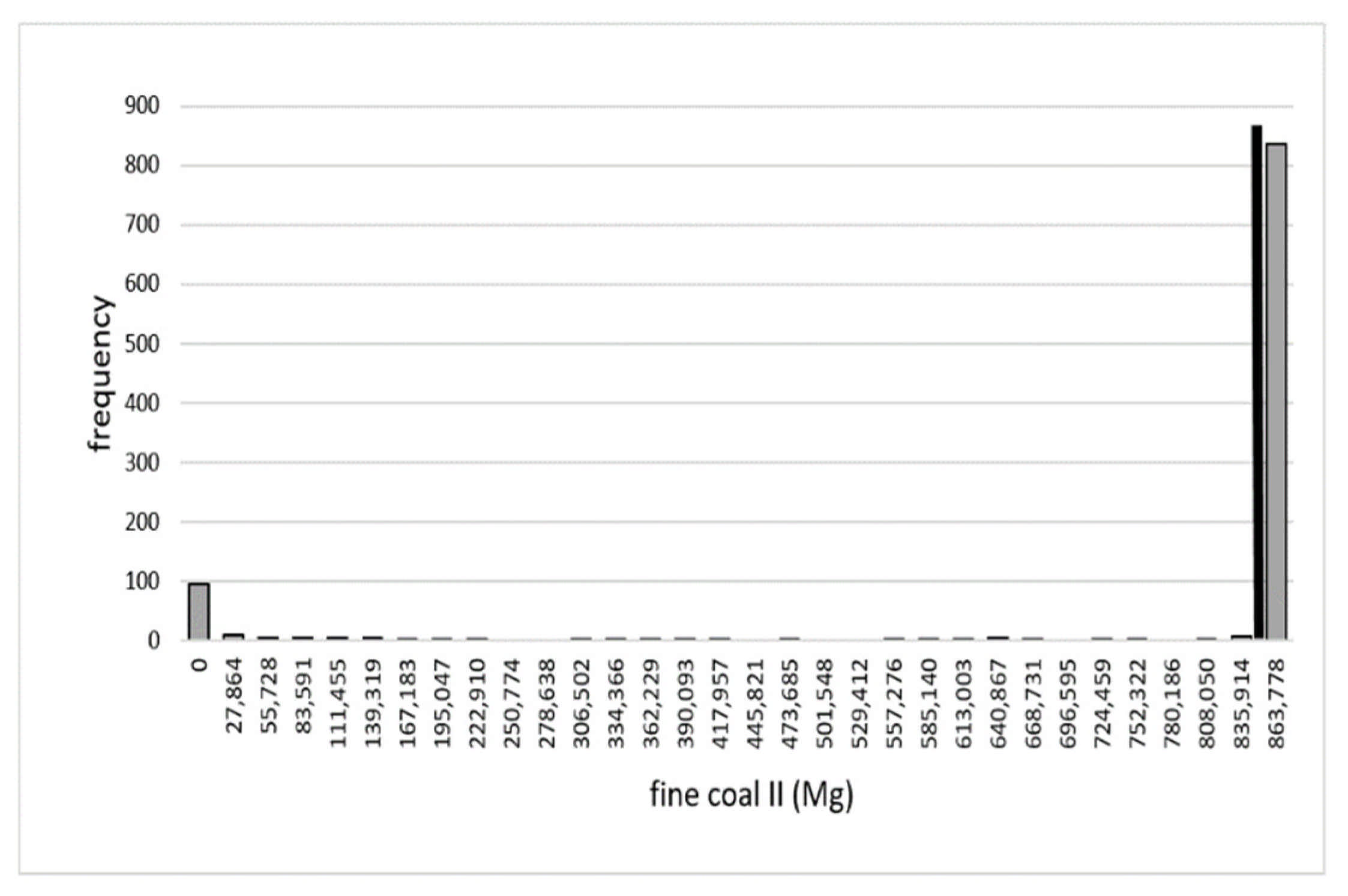
Energies 14 07111 g0a1
Figure A2. Histogram showing frequencies of achieving given quantity of sales fine coal II for mine “A” with σyprog.
Energies 14 07111 g0a2
Figure A3. Histogram showing frequencies of achieving given quantity of sales slurry for mine “A” with σyprog.
Energies 14 07111 g0a3
Figure A4. Histogram showing frequencies of achieving given quantity of sales of coking coal for mine “B” with σyprog.
Energies 14 07111 g0a4
Figure A5. Histogram showing frequencies of achieving given quantity of sales of coking coal (“Export 5”) for mine “C” with σyprog.
Energies 14 07111 g0a5
Figure A6. Histogram showing frequencies of achieving given quantity of sales of coking coal (“Cokerys 3”) for mine “C” with σyprog.
Energies 14 07111 g0a6
Figure A7. Histogram showing frequencies of achieving given quantity of sales of cobble for mine “D” with σyprog.
Energies 14 07111 g0a7
Figure A8. Histogram showing frequencies of achieving given quantity of sales of fine coal II for mine “D” with σyprog.
Energies 14 07111 g0a8
Figure A9. Histogram showing frequencies of achieving given quantity of sales of fine coal IIA (“Indv. Consumers 2”) for mine “D” with σyprog.
Energies 14 07111 g0a9
Figure A10. Histogram showing frequencies of achieving given quantity of sales of fine coal IIA (“Chamber grates 1”) for mine “D” with σyprog.
Energies 14 07111 g0a10
Figure A11. Histogram showing frequencies of achieving given quantity of sales of coking coal (“Export 2”) for mine “D” with σyprog.
Energies 14 07111 g0a11
Figure A12. Histogram showing frequencies of achieving given quantity of sales of coking coal (“Export 3”) for mine “D” with σyprog.
Energies 14 07111 g0a12
Figure A13. Histogram showing frequencies of achieving given quantity of sales of coking coal (“Cokerys 1”) for mine “D” with σyprog.
Energies 14 07111 g0a13
Figure A14. Histogram showing frequencies of achieving given quantity of sales of cobble for mine “E” with σyprog.
Energies 14 07111 g0a14
Figure A15. Histogram showing frequencies of achieving given quantity of sales of nut coal for mine “E” with σyprog.
Energies 14 07111 g0a15
Figure A16. Histogram showing frequencies of achieving given quantity of sales of fine coal I for mine “E” with σyprog.
Energies 14 07111 g0a16
Figure A17. Histogram showing frequencies of achieving given quantity of sales of fine coal II for mine “E” with σyprog.
Energies 14 07111 g0a17
Figure A18. Histogram showing frequencies of achieving given quantity of sales of slurry (“Grates 2”) for mine “E” with σyprog.
Energies 14 07111 g0a18
Figure A19. Histogram showing frequencies of achieving given quantity of sales of slurry (“Chamber grates 2”) for mine “E” with σyprog.
Energies 14 07111 g0a19
Figure A20. Histogram showing frequencies of achieving given quantity of sales of coking coal (“Export 1”) for mine “E” with σyprog.
Energies 14 07111 g0a20
Figure A21. Histogram showing frequencies of achieving given quantity of sales of coking coal (“Export 2”) for mine “E” with σyprog.
Energies 14 07111 g0a21
Figure A22. Histogram showing frequencies of achieving given quantity of sales of cobble for mine “G” with σyprog.
Energies 14 07111 g0a22
Figure A23. Histogram showing frequencies of achieving given quantity of sales of fine coal II (“Dust kettles”) for mine “G” with σyprog.
Energies 14 07111 g0a23
Figure A24. Histogram showing frequencies of achieving given quantity of sales of fine coal IIA (“Export 9”) for mine “G” with σyprog.
Energies 14 07111 g0a24
Figure A25. Histogram showing frequencies of achieving given quantity of sales of fine coal IIA (“Indv. consumers 2”) for mine “G” with σyprog.
Energies 14 07111 g0a25
Figure A26. Histogram showing frequencies of achieving given quantity of sales of fine coal IIA (“Dust kettles”) for mine “G” with σyprog.
Energies 14 07111 g0a26
Figure A27. Histogram showing frequencies of achieving given quantity of sales of fine coal II (“Export 7”) for mine “G” with σyprog.
Energies 14 07111 g0a27
Figure A28. Histogram showing frequencies of achieving given quantity of sales of slurry for mine “G” with σyprog.
Energies 14 07111 g0a28

References

  1. Hippert, H.S.; Pedreira, C.E.; Souza, R.C. Neural networks for short-term load forecasting: A review and evaluation. IEEE Trans. Power Syst. 2001, 16, 44–55. [Google Scholar] [CrossRef]
  2. Kaminski, V. The challenge of pricing and risk managing electricity derivatives. In The US Power Market; Barber, P., Ed.; Risk Books: London, UK, 1997. [Google Scholar]
  3. Bunn, D. Forecasting loads and prices in competitive power markets. Proc. IEEE 2000, 88, 163–169. [Google Scholar] [CrossRef]
  4. Nowicka-Zagrajek, J.; Weron, R. Modeling electricity loads in California: ARMA models with hyperbolic noise. Signal Process. 2002, 82, 1903–1915. [Google Scholar] [CrossRef] [Green Version]
  5. Sadownik, R.; Barbosa, E.P. Short-term forecasting of industrial electricity consumption in Brasil. J. Forecast. 1999, 18, 215–224. [Google Scholar] [CrossRef]
  6. Smith, M. Modeling and short-term forecasting of New South Wales electricity system load. J. Bus. Econom. Stat. 2000, 18, 465–478. [Google Scholar] [CrossRef]
  7. Larose, D.T. Data Mining Methods and Models; Wiley-Interscience Publication: Hoboken, NJ, USA, 2006. [Google Scholar]
  8. Box, G.P.; Jenkins, G.M. Analiza Szeregów Czasowych. Prognozowanie i Sterowanie; PWN: Warszawa, Poland, 1983. (In Polish) [Google Scholar]
  9. Michieka, N.M.; Fletcher, J. An investigation of the role of China’s urban population on coal consumption. Energy Policy 2012, 48, 668–676. [Google Scholar] [CrossRef]
  10. Chong, C.; Ma, L.; Li, Z.; Ni, W.; Song, S. Logarithmic mean Divisia index (LMDI) decomposition of coal consumption in China based on the energy allocation diagram of coal flows. Energy 2015, 85, 366–378. [Google Scholar] [CrossRef]
  11. Lin, B.; Wu, W. Coal demand in China’s current economic development. China Soc. Sci. 2018, 2, 141–161. [Google Scholar]
  12. Vaziri, M.; Hutchinson, J. Short-run forecasting of United States coal production. Int. J. Min. Geol. Eng. 1987, 5, 419–432. [Google Scholar] [CrossRef]
  13. Yawei, O.; Li, O. A forecast of coal demand based on the simultaneous equations model. In Proceedings of the 2011 IEEE International Symposium on IT in Medicine and Education, Guangzhou, China, 9–11 December 2012. [Google Scholar]
  14. Zhu, Q.; Zhang, Z.; Chai, J.; Wang, S. Coal demand forecasting model based on consumption structure division. Syst. Eng. 2014, 32, 112–123. [Google Scholar]
  15. Jebaraj, S.; Iniyan, S.; Goic, R. Forecasting of Coal Consumption Using an Artificial Neural Network and Comparison with Various Forecasting Techniques. Energy Sources Part A Recovery Environ. Eff. 2011, 33, 1305–1316. [Google Scholar] [CrossRef]
  16. Rybak, A.; Manowska, A. Zjawisko sezonowości popytu a strategie produkcji węgla kamiennego w Polsce. Zeszyty Naukowe Politechniki Śląskiej 2017, 108, 373–382. (In Polish) [Google Scholar]
  17. Barnett, V. Elementy Pobierania Prób; PWN: Warszawa, Poland, 1982. (In Polish) [Google Scholar]
  18. Bobrowski, D. Probabilistyka w Zastosowaniach Technicznych; WNT: Warszawa, Poland, 1986. (In Polish) [Google Scholar]
  19. Brandt, S. Analiza Danych. Metody Statystyczne i Obliczeniowe; PWN: Warszawa, Poland, 1998. (In Polish) [Google Scholar]
  20. Brockwell, P.J.; Davis, R. Introduction to Time Series and Forecasting; Springer: New York, NY, USA, 2002. [Google Scholar]
  21. Fishman, G.S. Monte Carlo: Concepts, Algorithms and Applications; Springer: New York, NY, USA, 1996. [Google Scholar]
  22. Zieliński, R. Metoda Monte Carlo; WNT: Warszawa, Poland, 1974. (In Polish) [Google Scholar]
  23. Fuksa, D. The ways of solving non-linear decision problems through application of optimal production plans for mines/Sposoby rozwiązywania nieliniowych problemów decyzyjnych w opracowywaniu optymalnych planów produkcji kopalń. Min. Res. Man. 2007, 23, 97–108. (In Polish) [Google Scholar]
  24. Fuksa, D. The method for the assessment of the impact of variable demand of hard coal consumers on the profitability of a multi-facility mining enterprise/Metoda oceny wpływu zmiennego zapotrzebowania odbiorców węgla na rentowność wielozakładowego przedsiębiorstwa górniczego. Inżynieria Miner. 2017, 1, 249–256. (In Polish) [Google Scholar]
  25. Fuksa, D. Consolidation of mining enterprises as a chance to make the Polish mining industry profitable. Inżynieria Miner. 2018, 2, 47–54. [Google Scholar] [CrossRef]
  26. Bendkowski, J. Zarządzanie operacyjne—Istota, zakres przedmiotowy. Zeszyty Naukowe Politechniki Śląskiej. Organ. i Zarz. 2004, 21, 7–17. [Google Scholar]
  27. Błażewicz, J. Badania Operacyjne Dla Informatyków; WNT: Warszawa, Poland, 1983. (In Polish) [Google Scholar]
  28. Gal, T. Betriebliche Entscheidungsprobleme, Sensitivitätalise Sensitivitätsanalyse und Parametrische Programmierung; Gruyter: Berlin, Germany, 1973. [Google Scholar]
  29. Grabowski, W. Programowanie Matematyczne; PWN: Warszawa, Poland, 1982. (In Polish) [Google Scholar]
  30. Grudzewski, W. Badania Operacyjne w Organizacji i Zarządzaniu; PWN: Warszawa, Poland, 1985. (In Polish) [Google Scholar]
  31. Gruszczyński, M.; Podgórska, M. Ekonometria; SGH: Warszawa, Poland, 1996. (In Polish) [Google Scholar]
  32. Ignasiak, E. Badania Operacyjne; PWN: Warszawa, Poland, 1996. (In Polish) [Google Scholar]
  33. Miszczyński, M. Programowanie Liniowe; Przedsiębiorstwo Specjalistyczne “Absolwent”: Łódź, Poland, 1997. (In Polish) [Google Scholar]
  34. Nykowski, I. Programowanie Liniowe; PWN: Warszawa, Poland, 1980. (In Polish) [Google Scholar]
  35. Fuksa, D. Racjonalizacja Decyzji Produkcyjnych w Spółce Węglowej z Wykorzystaniem Analizy Postoptymalnej; Wydawnictwa AGH: Kraków, Poland, 2016. (In Polish) [Google Scholar]
  36. Lisowski, A.; Czylok, A. Możliwości wykorzystania metod i modeli matematycznych oraz symulacyjnych do optymalizacji decyzji w górnictwie. Przegląd Górniczy 1965, 6, 276–285. [Google Scholar]
  37. Oktaba, W. Elementy Statystyki Matematycznej i Metodyka Doświadczalnictwa; PWN: Warszawa, Poland, 1980. (In Polish) [Google Scholar]
  38. Snopkowski, R. Boundary conditions for elementary functions of probability densities for the production process realised in longwalls. Arch. Min. Sci. 2000, 45, 501–510. [Google Scholar]
  39. Nowak, E. Zaawansowana Rachunkowość Zarządcza; PWE: Warszawa, Poland, 2003. (In Polish) [Google Scholar]
  40. Samuelson, W.F.; Marks, S.G. Ekonomia Menadżerska; PWN: Warszawa, Poland, 1998. (In Polish) [Google Scholar]
  41. Goryl, A.; Jędrzejczyk, Z. Wprowadzenie do Ekonometrii w Przykładach i Zadaniach; PWN: Warszawa, Poland, 1996. (In Polish) [Google Scholar]
  42. Gnot, S. Estymacja Komponentów Wariancyjnych w Modelach Liniowych; WNT: Warszawa, Poland, 1991. (In Polish) [Google Scholar]
  43. Grabiński, T.; Wydymus, S.; Zaliaś, A. Metody Doboru Zmiennych w Modelach Ekonometrycznych; PWN: Warszawa, Poland, 1982. (In Polish) [Google Scholar]
  44. Grabiński, T.; Wydymus, S.; Zaliaś, A. Modele Ekonometryczne w Procesie Prognozowania; AE: Kraków, Poland, 1978. (In Polish) [Google Scholar]
Figure 1. The flowchart of the algorithm of the proposed method.
Energies 14 07111 g001
Figure 2. The SIMPLEX algorithm flowchart with the maximization of the objective function.
Energies 14 07111 g002
Figure 3. Demand of the “Indv. consumers 1” group in the years 2010–2020 with the forecast for 2021.
Energies 14 07111 g003
Figure 4. Demand of the “Export 1” group in the years 2014–2020 with the forecast for 2021.
Energies 14 07111 g004
Figure 5. Demand of the “Export 7” group in the years 2014–2020 with the forecast for 2021.
Energies 14 07111 g005
Figure 6. Histogram showing frequencies of achieving given profits for mine “F” with dispersion σyprog. * The black vertical line illustrates the nominal value quantity (according to the optimal plan from Table 10).
Energies 14 07111 g006
Figure 7. Histogram showing frequencies of achieving given quantity of sales of cobble for mine “F” with σyprog.
Energies 14 07111 g007
Figure 8. Histogram showing frequencies of achieving given quantity of sales of coal for mine “F” with σyprog.
Energies 14 07111 g008
Figure 9. Histogram showing frequencies of achieving given quantity of sales of coking coal for mine “F” with σyprog.
Energies 14 07111 g009
Table 1. Technical and economic coefficients for mines.
MinesAverage ExtractionMax. ExtractionUnit CostFixed Cost
(Mg/day)(Mg/year)(PLN/Mg)(%)
Mine A55001,454,750131.20 (EUR 27.71)69.51
Mine B3000793,500139.40 (EUR 30.50)72.22
Mine C4200966,000132.68 (EUR 29.03)68.95
Mine D12,0002,760,000136.50 (EUR 29.86)73.40
Mine E11,3002,599,000137.20 (EUR 30.02)71.31
Mine F12,8003,385,600138.30 (EUR 30.26)69.37
Mine G11,5002,645,000134.40 (EUR 29.41)69.38
Table 2. Types and quality parameters of coal offered by mines.
MinesCoal Size GradeCoal Type NameShare in ExtractionCalorific Value
(%)(kJ/kg)
Mine Acobble3311.024,892
nut coal331.525,650
fine coal I3318.225,904
fine coal IIA32.146.420,089
fine coal II32.121.822,056
slurry32.11.113,516
Mine Bfine coal II32.131.022,142
coking coal34.169.028,789
Mine Ccoking coal34.1100.031,552
Mine Dcobble332.229,504
nut coal330.526,988
fine coal IIA3340.7422,233
fine coal II34.21.129,924
coking coal34.255.4628,884
Mine Ecobble337.231,189
nut coal331.329,520
fine coal I32.26.925,600
fine coal IIA32.151.720,788
fine coal II32.128.924,533
slurry-2.915,722
coking coal34.21.128,936
Mine Fcobble337.1930,238
nut coal331.829,268
fine coal I32.27.1928,780
fine coal IIA32.10.720,667
fine coal II32.165.0422,813
slurry-2.216,487
coking coal34.215.8828,455
Mine Gcobble333.4930,283
nut coal330.529,934
fine coal I330.3928,746
fine coal IIA3352.922,720
fine coal II32.16.723,255
slurry-1.118,305
coking coal34.234.9228,941
Table 3. The characteristics of the company’s aggregated consumer groups.
Name of Consumer GroupAccepted Types of Coal 1
1234567891011121314151617
Export 1 x
Export 2 x
Export 3 x
Export 4 xx
Export 5 xxxx
Export 6 xxxx
Export 7 xxxx
Indv. consumers 1 xxxx
Indv. consumers 2 xxxx
Cokerys 1 xx
Cokerys 2 xxx
Cokerys 3 xxxxx
Dust kettles xxxxxxx
Grates 1x xxx
Grates 2xxxxxxxxxxxxxxxxx
Chamber grates 1x xxx
Chamber grates 2 xxx
1 see Table 5.
Table 4. The characteristics of the company’s aggregated consumer groups.
Name of Consumer GroupAccepted Assortment NameDemandMaximum Calorific ValueMinimum Calorific Value
123456789(Mg/year)(kJ/kg)(kJ/kg)
Export 1 x24,92029,30825,960
Export 2 x328,08241,86825,960
Export 3 x239,01541,86823,027
Export 4 x133,94441,86823,027
Export 5x 243,95529,30725,958
Export 6 xx 92,95926,79525,120
Export 7 xxx 1,235,01325,12023,027
Indv. consumers 1xxx 336,71429,30720,934
Indv. consumers 2 xxx 1,368,04625,12020,934
Cokerys 1 x676,32341,86824,900
Cokerys 2 x81,28441,86824,900
Cokerys 3 x900,67641,86824,900
Dust kettles xxx 5,907,55023,02712,979
Grates 1 xx 126,78918,84014,653
Grates 2 xxx 65,72418,84014,653
Chamber grates 1 xxx 49,29921,77119,259
Chamber grates 2 xxx 38,28618,84014,653
1 see Table 5.
Table 5. List of numbers and names of coal types.
Coal Type/Assortment NumberCoal Type NameAssortment Name
131.1cobble
231.2nut coal
332.1fine coal I
432.2fine coal II
533fine coal IIA
634.1slurry
734.2coking coal
835.1
935.2A
1035.2B
1136
1237.1
1337.2
1438
1541
1642
1743
Table 6. A summary of the nominal values of the forecast of the demand from the consumer groups and of the dispersion σyprog.
Name of Consumer GroupNominal Prognosis ValuesDispersion σyprog
(Mg)(Mg)
Export 124,9201,675.30
Export 2328,08222,056.13
Export 3239,01516,068.36
Export 4133,9449004.69
Export 5243,95516,400.50
Export 692,9596249.39
Export 71,235,01383,026.78
Indv. consumers 1336,71418,924.03
Indv. consumers 21,368,04681,045.96
Cokerys 1676,32335,788.92
Cokerys 281,2844301.29
Cokerys 3900,67647,660.97
Dust kettles5,907,550312,609.30
Grates 1126,7896709.27
Grates 265,7243477.92
Chamber grates 149,2992608.74
Chamber grates 238,2862025.96
Table 7. A summary of the regression analysis results for the domestic coal sales (“Indv. consumers 1”).
ModelThe Model form of the FunctionCorrelation Coefficient
linearZ = −13,035.91t + 493,145.06−0.939
exponentialZ = 500,842.61 × 0.968t−0.930
hyperbolicZ = 382,551.32 × 117,938.95/t0.691
powerZ = 506,073.86 × t−0.13−0.830
logarithmicZ = 498,617.53 − 121,108.83logt−0.851
Table 8. A summary of the regression analysis results for the domestic coal sales (“Export 1”).
ModelThe Model form of the FunctionCorrelation Coefficient
linearZ = −1935.06t + 40,400.33−0.9631
exponentialZ = 41,160.05 × 0.94t−0.9629
hyperbolicZ = 28,284.87 × 11,811.94/t0.8249
powerZ = 40,290.10 × t−0.18−0.9129
logarithmicZ = 39,792.53 − 13,484.91logt−0.9240
Table 9. A summary of the regression analysis results for the domestic coal sales (“Export 7”).
ModelThe Model form of the FunctionCorrelation Coefficient
linearZ = −104,292.09t + 2,047,921.34−0.978
exponentialZ = 2,093,621.65 × 0.94t−0.975
hyperbolicZ = 1,403,079.82 × 614,654.82/t0.809
powerZ = 2,041,275.94 × t−0.19−0.916
logarithmicZ = 2,011,000.32 − 718,914.59logt−0.928
Table 10. The optimal production and sales plan for mine “F” for 2021.
Name of Consumer GroupCoal Size GradeSales QuantityTotal SalesProfit:Mine Reserves
(Mg)(Mg)(PLN)(Mg)
Export 5cobble225,0123,069,123395,060,7480
Cokerys 2coking coal78,136 (EUR 86,446,553)
Export 6nut coal46,885
Indv. consumers 1cobble18,507
Cokerys 1coking coal231,563
Dust kettlesfine coal I243,520
Dust kettlesfine coal IIA23,675
Dust kettlesfine coal II2,201,825
Dumping coalcoking coal228,073
Dumping coalnut coal13,995
Dumping coalslurry74,409
Table 11. A summary of the expected gross profit with the probability of achieving them at σyprog for mine “F”.
Nominal ProfitMinimum ProfitMaximum ProfitProbability of Achieving
Nominal ProfitMinimum ProfitMaximum Profit
(PLN)(PLN)(PLN)(-)(-)(-)
99,053,000
(EUR 21,674,617)
46,437,497
(EUR 10,161,378)
149,825,520
(EUR 32,784,577)
0.48210.181
Table 12. A summary of the volumes of sales of the individual coal grades with the probability of their achievement at σyprog for mine “F”.
Coal Size GradeQuantity According to PlanMinimum QuantityMaximum QuantityProbability of Achieving
the Quantity
According to the Planminmax
(Mg)(Mg)(Mg)(-)(-)(-)
cobble243,519228,456243,5190.99810.998
nut coal46,88524,85360,8800.58610.071
fine coal I243,519243,519243,519111
fine coal IIA23,67523,67523,675111
fine coal II2,201,8252,201,8252,201,825111
coking coal251,2400537,7720.5320.6760.352
Publisher’s Note: MDPI stays neutral with regard to jurisdictional claims in published maps and institutional affiliations.

