Abstract
Knowledge of a direct-drive model with a complex mechanical part is important in the synthesis of control algorithms and in the predictive maintenance of digital twins. The identification of two-mass drive systems with one low mechanical resonance frequency is often described in the literature. This paper presents an identification workflow of a multi-resonant mechanical part in direct drive with up to three high-frequency mechanical resonances. In many methods, the identification of a discrete time (DT) model is applied, and its results are transformed into a continuous-time (CT) representation. The transformation from a DT model to a CT model has limitations due to nonlinear mapping of discrete to continuous frequencies. This problem may be overcome by identification of CT models in the frequency domain. This requires usage of a discrete Fourier transform to obtain frequency response data as complex numbers. The main work presented in this paper is the appropriate fitting of a CT model of a direct-drive mechanical part to complex number datasets. Fitting to frequency response data is problematic due to the attraction of unexcited high frequency ranges, which lead to wrong identification results of multi-mass (high order) drive systems. Firstly, a CT fitting problem is a nonlinear optimization problem, and, secondly, complex numbers may be presented in several representations, which leads to changes in the formulation of the optimization problem. In this paper, several complex number representations are discussed, and their influence on the optimization process by simulation evaluation is presented. One of the best representations is then evaluated using a laboratory setup of direct drive with unknown parameters of three high mechanical resonance frequencies. The mechanical part of the examined direct drive is described by three mechanical resonances and antiresonances, which are characteristic of a four-mass drive system. The main finding is the addition of frequency boundaries in the identification procedure, which are the same as those in the frequency range of the excitation signal. Neither a linear least-square algorithm nor a nonlinear least-square algorithm is suitable for this approach. The usage of nonlinear least-square algorithm with constraints as a fitting algorithm allows one to solve the issue of modeling multi-mass direct-drive systems in the frequency domain. The second finding of this paper is a comparison of different cost functions evaluated to choose the best complex number representation for the identification of multi-mass direct-drive systems.
1. Introduction
Knowledge of the electromechanical system model is important for many different reasons. It provides information regarding both the structure and parameters of the real system from the model point of view. This assists in understanding electromechanical system dynamic behavior in many practical cases. It also provides a tool to the simulate behavior of the electromechanical system in different conditions [1,2]. Deep knowledge of the model will be helpful in selecting a classical control method and tuning it and using a predictive control algorithm [3,4] or one of the adaptive control methods [2,5,6]. Another wide range of applications that are based on model knowledge are fault diagnosis methods, where the model is used to calculate residuum between the model and the real system.
Mechatronic systems with a resonant mechanical part are difficult to control and are interesting subjects for many researchers worldwide. The difficulty is associated with the number of mechanical resonances and their frequencies. Mechatronic systems with one mechanical resonance (a two-mass drive system) and low frequency have been evaluated in recent years. This includes an example of one mechanical resonance (two-mass drive system) from 10.2 to 17.6 [7], 9.6 [8], and 70 Hz [9]. The identification of two-mass drive systems has also been the subject of research. Online estimation of one mechanical resonance in the range of 54–80 Hz using pseudo-random binary signal (PRBS) and discrete-time transfer function (DTTF) was carried out in [10] and in the range of 54–91 Hz using a chirp signal and DTTF model in [11]. Furthermore, there has been identification of a resonating mechanical system in mobile road vehicles modeled as two-mass systems (one mechanical resonance of about 12 Hz) using PRBS, chirp, and stepped sine signals [12]. The PRBS excitation signal was also used in [13] to identify two-mass model parameters based on a DTTF model. The article [13] also presents identification of two-mass mechanical systems with one mechanical resonance of about 80 Hz using PRBS and DTTF models. The identification of a drive system with one (64 or 100 Hz) and two mechanical resonance frequencies (around 60 and 100 Hz) was studied in [14] using PRBS and a continuous-time model, with the cost function calculated as a module of the difference between the sampled frequency response and continuous-time model.
Previous research has focused on multi-mass drive systems with high mechanical resonance frequencies in ranges up to 500 Hz. The first approach of the author of [15] used only output signal in frequency domains with a custom search algorithm. The dynamic search algorithm assists in finding appropriate resonance frequencies without a system model and an unknown number of resonances. However, anti-resonance frequencies were not identified by this algorithm, and a second drawback is its accuracy of around ±3 Hz. This algorithm was successfully tested and compared [3] with manual identification used in control systems, with variable mechanical parameters with three resonance frequencies of 105, 251, and 417 Hz. Research was carried out by the author of [16] to compare the identification of one resonance system in simulation and to identify laboratory setups with three mechanical resonances using PRBS and chirp signals as input and different means of identification of DTTF models (ARX—autoregressive with exogenous input and OE—output error). The usage of ARX and OE DTTF models gives fair results of identification and underlines the problem of the attraction of model parameters to high-frequency components by using a linear least-squares algorithm. In the next stage of development in this field of research, a nonlinear least-squares algorithm was used by the author of [17] to find parameters that best fit frequency response data. The obtained identification results were positive only for the first two resonances of 81 and 202 Hz, without appropriate identification of the higher resonance component at 273 Hz because of the attraction of high-frequency components above the cutoff frequency of the current control loop. Studies [15,16,17] showed that chirp signals give a smoother frequency response in comparison to PRBS, as the frequency range is banded and the magnitude is flat. A second conclusion from previous work is that linear least-squares with the DTTF model and nonlinear-least squares methods with the continuous-time transfer function model are attracted by higher frequency parts of the frequency response.
In this article, the author focuses on multi-mass drive systems with high frequencies. The laboratory stand is characterized by three main mechanical resonance frequencies in ranges of up to 500 Hz. The difficulty of the subject increases by the number of resonance frequencies, where tree mechanical resonances are characteristic of a four-mass system. Another difficulty is their high frequency values close to a region that exhibits no excitement in the frequency domain. The main finding of this article is the identification of a direct-drive system with a complex mechanical part, characterized by high frequency resonances as a continuous-time model directly within a frequency domain. Previous research has used a known nonlinear least-squares algorithms without constraints for less complex mechanical systems in a lower frequency range. This article shows the usage of a nonlinear least-squares algorithm with constraints to handle high-frequency attraction problems in the direct-drive system. The secondary findings presented in this article describe differences in cost functions based on complex number representation in the direct-drive system.
In practice, algorithms used for control and monitoring of electromechanical systems run on microcontrollers, or microprocessors, which process data with a constant sample time and with a limited bit resolution. Therefore, the data used for the model design will have constraints of value and time resolution. The model will be identified using sampled data; however, the model representation can still be chosen.
Model structure can be selected arbitrarily based on designer experience or by an algorithm. The first step of the identification workflow is to select a representation of the model structure. Classical identification methods use a discrete-time (DT) model structure and sampled data. In this paper, a continuous-time (CT) model structure processing sampled data is considered. CT system identification in the time domain requires special treatment of time derivatives [18]. A suitable model of an electric drive with a multi-resonant mechanical part may be prepared in several model representations [19]. If the mechanical part construction is known and well described by the equations of motion, the most suitable representation will be continuous-time state space (CTSS) with selected space variables. In practice, CTSS has multiple outputs and multiple inputs, but electric motor velocity and load velocity are most commonly selected as the outputs, and electric motor torque and load torque are selected as the inputs. Multi-input multi-output (MIMO) CTSS model representation can be transformed into a matrix of several continuous-time Laplace transfer functions (CTTF), where one CTTF describes the dynamic relationship of single input and single output (SISO), with zero condition of the other inputs [19].
The next step of the identification workflow is the selection of inputs and outputs of an electric drive with a multi-resonant mechanical part, which are used further in the procedure. In real-world applications, not all inputs and outputs are available or measurable. Therefore, an MIMO model is constructed on a limited number of SISO sampled data. In this paper, the measured electric motor velocity and the current controller setpoint corresponding to the torque of the electric motor are used.
The final step is fitting the model to the measured data and validating the obtained results. This leads to a model fitting problem known in machine learning and curve fitting methods. One issue of fitting a model to measured sampled data is the optimization problem. If model parameters are bounded, there can be an optimization problem with constraints. Optimization solvers are a well known and present large group of methods, such as linear programming, quadratic programming, nonlinear programming, linear least squares, and nonlinear least squares [20]. The identification of a discrete model from sampled time-domain data can be applied by linear programing [13,16]; however, in this approach, transformation to continuous representation after identification is required, and this method lacks frequency constraints. Many different methods have been developed to identify CT based on time-domain data [18,21,22,23,24] or based on frequency-domain data [25,26,27,28]. As a fitting algorithm in the frequency domain, the methods of instrumental variable and linear least squares approximations [28], instrumental variable and bi-orthonormal polynomial bases [27], maximum likelihood [25], and weighted nonlinear least squares [26] have been applied.
In this paper, the nonlinear least-squares (NLS) method with constraints is applied to solve a nonlinear optimization problem of fitting the model to the frequency response dataset. Different complex number representations of the same datasets of frequency response data are thoroughly presented. All presented complex number representations are compared in a simulation test repeated one thousand times at different starting points. This allows for quality indicators of each representation to be prepared. A further novelty of the article is in bounding the NLS operating with frequency data to a specific range of frequencies of the excitation signal. A second constraint is added to the damping factor, so its assumed range is from zero to one. The presented identification workflow is verified by simulation and a dataset from the laboratory setup.
2. Frequency Model of Electric Drive with Multi-Resonant Mechanical Part
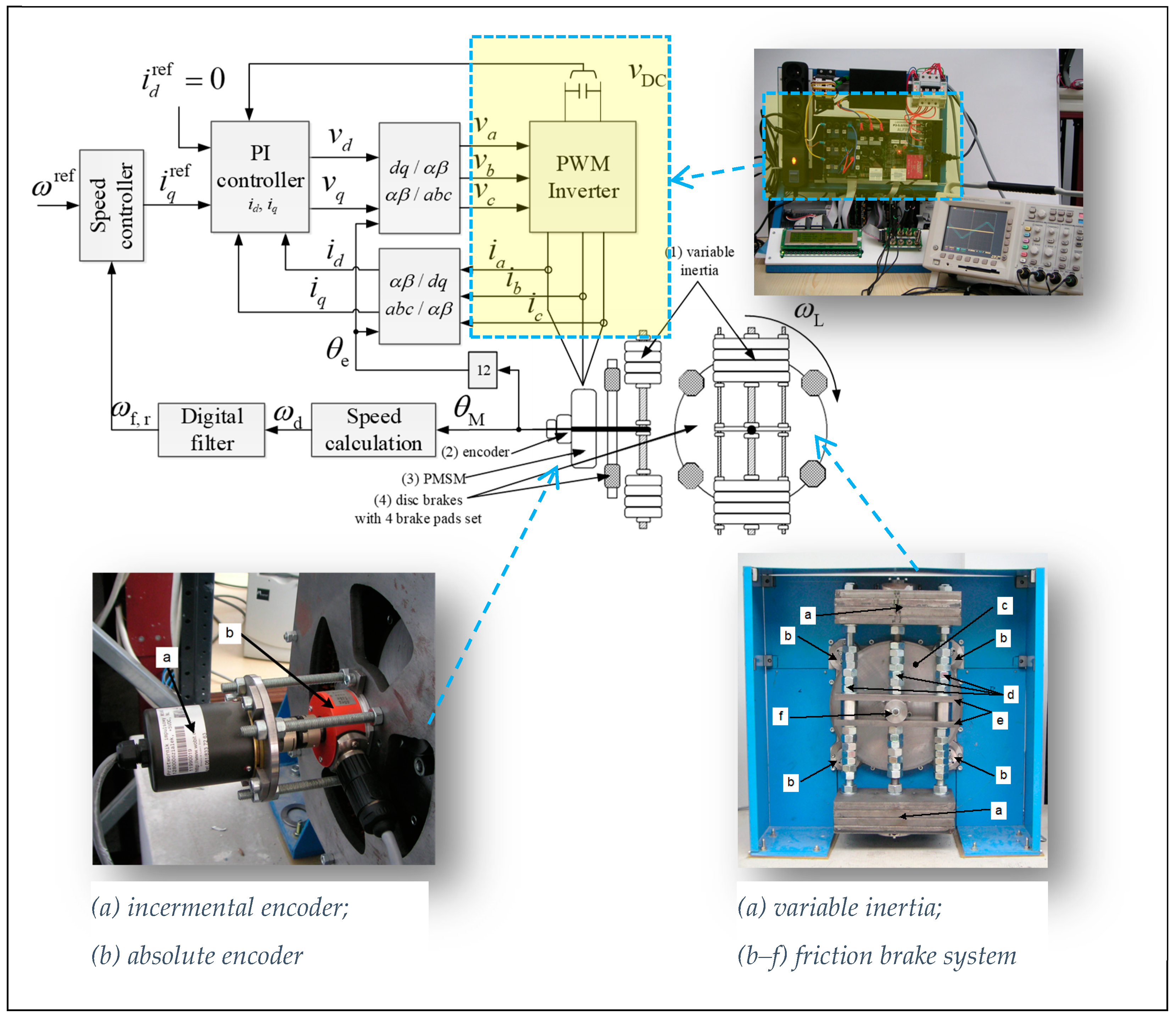
The model of the discussed electric direct drive has an electric part and a mechanical part. In the real application, a permanent magnet synchronous motor (PMSM) was used. The laboratory setup is presented in Figure 1. The electric part consisted of a 3-phase supply, a 3-phase rectifier, and a 3-phase inverter. The mechanical part consisted of metal plates directly mounted to the motor shaft. The laboratory setup allowed for the measurement of 3-phase currents and which are transformed to rotating coordinates and based on the rotor electric position which is calculated from the measured motor position multiplied by the number of motor pole pairs equal to 12. Two proportional–integral (PI) controllers were used to track reference currents and . Actuating signals are voltages in rotating coordinates and , transformed to 3-phase stationary coordinates , and as an input for a pulse-width modulation (PWM) inverter. The PWM switches voltage with a frequency of 10 kHz. The time constants of the electric part were significantly smaller than those of the mechanical part and had limited influence on the velocity and position of the mechanical part. In the current article, the author focused on the identification of the mechanical part with a known CTTF model of a current closed loop responsible for torque generation. The velocity of the motor was calculated from the motor angular position as a first time derivative , where is change in the motor angular position divided by change in time . The calculated velocity of motor contained high-frequency noise, and, therefore, a lowpass digital filter with a cutoff of 500 Hz frequency was applied. A low-pass filter is the first part of the digital filter shown in the diagram in Figure 1. The second part of the digital filter is a bandstop filter, tuned to attenuate resonance frequencies in feedback signal . The output of the used filter was used as a feedback signal in the speed controller with a reference velocity of . The velocity of the load is not available in the measurements.

Figure 1.
Laboratory stand setup and schematic.
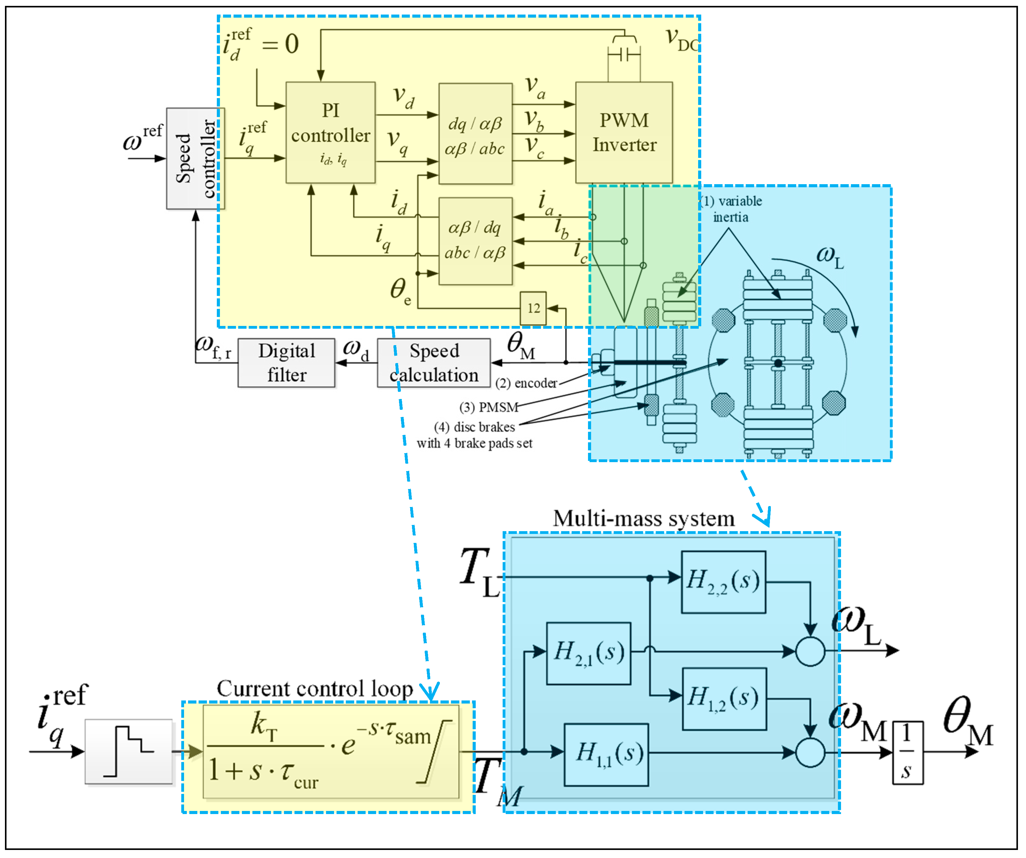
The mechanical part was modeled as four CTTFs: and , where only one pair of input and output was measurable, with motor current (equivalent to motor torque ) and motor velocity . The torque of load and the velocity of load were not measurable at the laboratory setup of direct drive. The model of the direct-drive mechanics is presented in Figure 2, where the current constant kT = 17.5 Nm/A, delays τcur = 300 μs, and τsam = 200 μs are known. The model of four CTTFs can be transformed to represent a MIMO-CTSS model if needed. At this point, a broader usage of the proposed method is worth mentioning. A reader who has a typical two-mass application [29] or a multi-mass application [3] can use the presented method after transforming CTSS to the matrix of CTTF. CTTF and relationships between motor current (equivalent to motor torque ) and motor velocity are described in (1).

Figure 2.
Simulation model of direct drive.
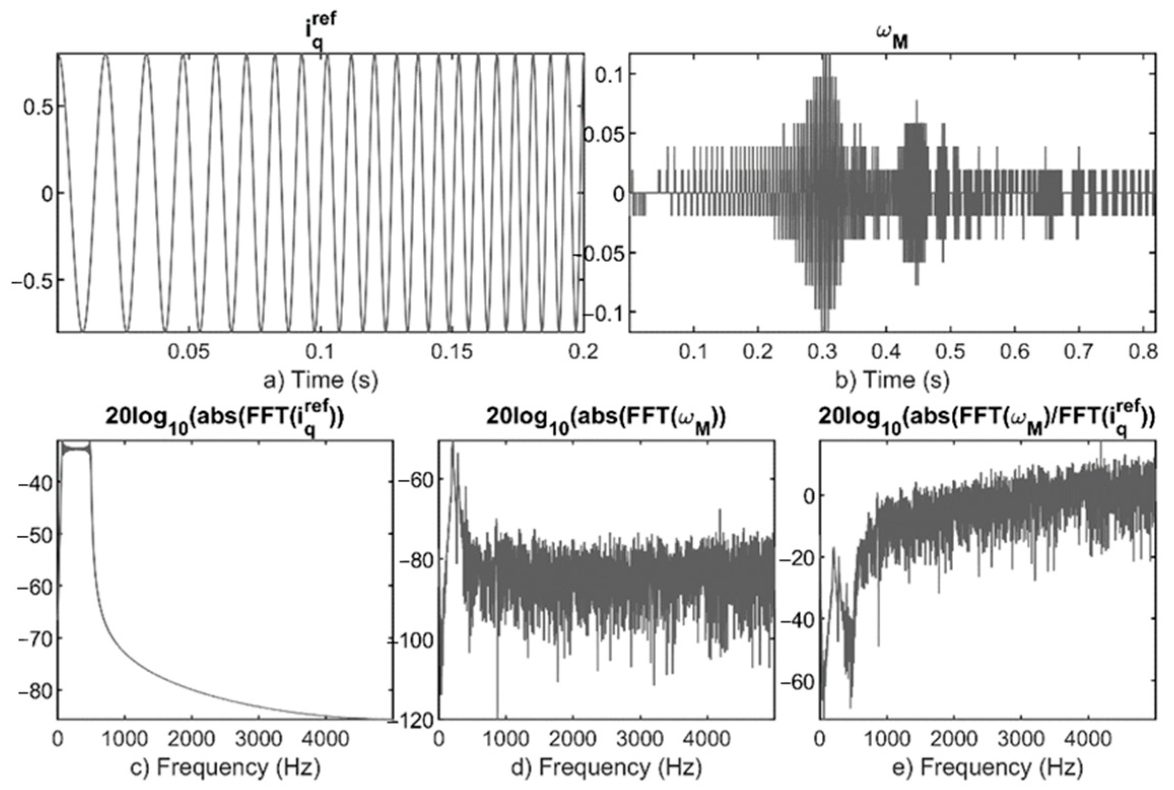
The Laplace CTTF model may be transformed into a continuous frequency response function (CFRF) by applying s = jω, where s is the Laplace operator and ω is the angular frequency (ω = 2πf, f—continuous frequency in Hz). In the result, (1) is transformed to (2). Sampled data (measurements) are delivered in the time domain and need to be transformed to the frequency domain by application of discrete Fourier transform (DFT). The transformed measurements were used to calculate discrete frequency response data (DFRD) by division of each complex number of the output and input. The CFRF model can be fitted to a complex number DFRD to find unknown parameters (3). In the real application, a linear chirp signal in the range of 50 to 500 Hz was used as the input, where change in frequency was achieved linearly in a time of 819.2 ms at the 100 μs sampling time. The linear chirp is a cosinusoidal signal with linearly increasing frequency in time. Part of the input signal change in time from 0 s to 200 ms is shown in Figure 3a, and the magnitude of the whole input signal is shown in Figure 3c. The linear chirp signal has flat magnitude characteristics and stimulates system frequencies equally in a selected frequency range (Figure 3c). The time domain input-output data and the magnitude of Fourier transform are presented in Figure 3. Figure 3b presents motor velocity calculated from the motor angular position as a first time derivative , where is changed by the motor angular position divided by change in time . The change in the angular position is considerably small in laboratory direct drive because of the used low-speed PMSM with 12 pole pairs. The nominal motor speed is 145 rpm. An applied encoder sensor has 125,000 impulses per revolution. The resolution was increased four times by counting both edges of signal channel A XOR B of the encoder. This setup allowed for safe excitation at a very low speed of drive without damage. Figure 3e presents DFRD of the laboratory direct drive in the frequency range from 0 to 5000 Hz (sampling frequency over two). The current control loop bandwidth of the laboratory stand is limited to about 530 Hz. Therefore, the part of DFRD above this frequency is useless because of a very small excitation that leads to an unreasonably large gain on output. The optimization of the model of resonance and anti-resonance frequencies was constrained to the range of the excitation spectrum.

Figure 3.
Data from the excitation procedure of direct drive. In the time domain: (a) excitation signal (input signal), (b) measured position (output signal); in the frequency domain: (c) amplitude spectrum of input, (d) amplitude spectrum of output, (e) frequency response data of direct drive.
3. Nonlinear Identification with Constraints in Frequency Domain
3.1. Identification from Synthetic Data
The examination of the CFRF model fitting to DFRD was carried out based on artificial data. This approach allowed for a synthetic selection of a mechanical structure (number of mechanical resonances) and the selection of its parameters. The most important feature in the synthetic variant is the possibility of verification of obtained parameters. In real application where the parameters and structure are unknown, validation is limited to numerical indicators, such as likelihood.
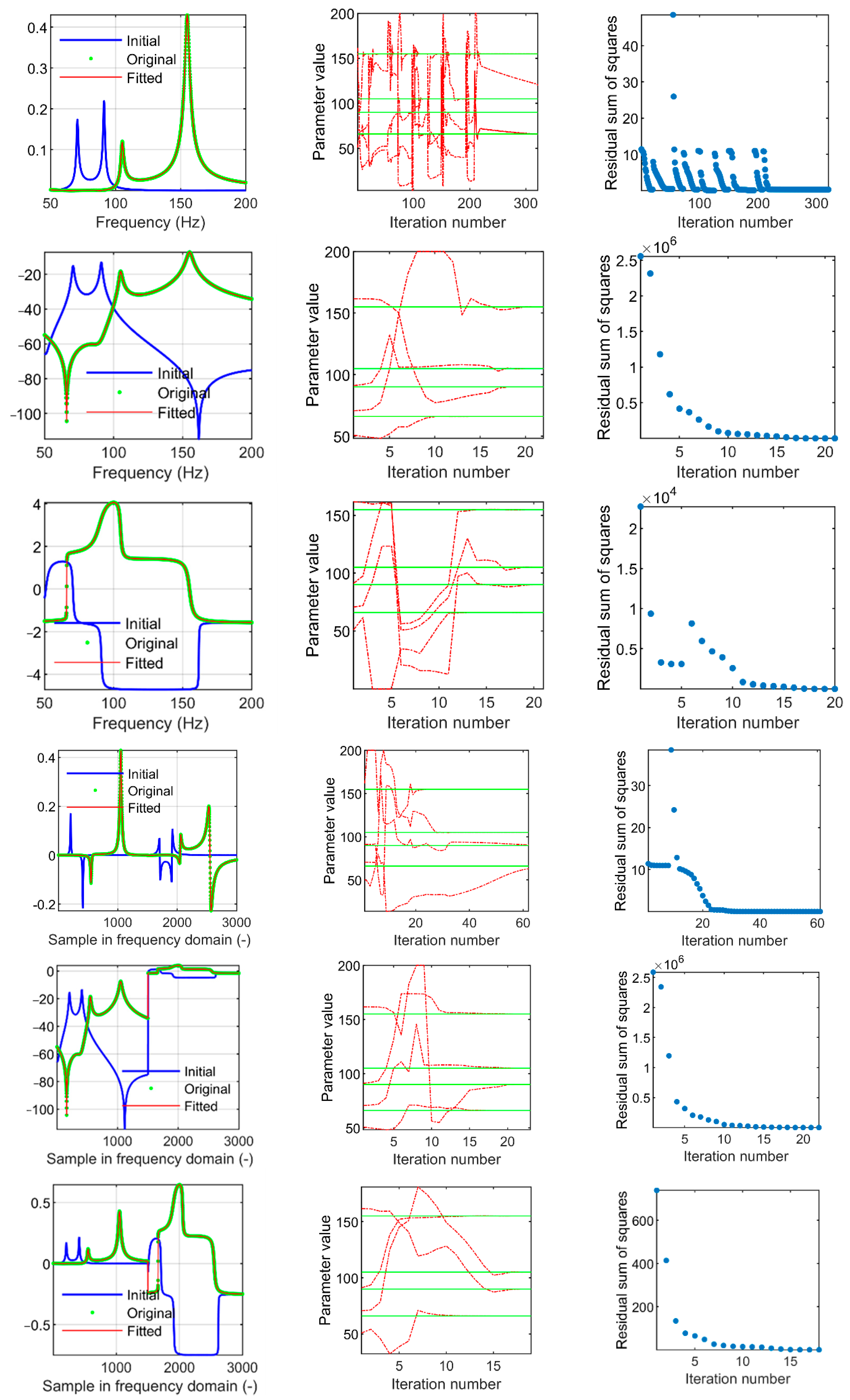
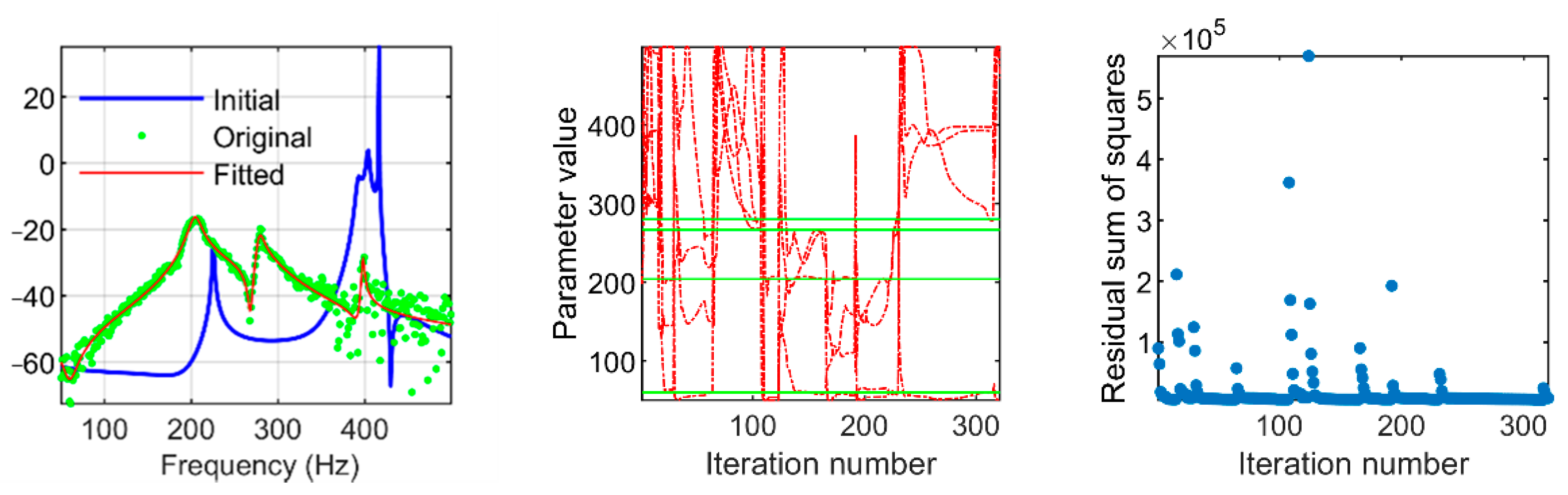
The frequency resolution of DFRD depends on the used sampling time and step of measurements. The synthetic data have a resolution of 0.1 Hz and frequency range () from 50 to 200 Hz, which gives 1500 complex numbers. DFRD is a vector of complex numbers, but most optimization solvers work in real numbers. In this work, the real number NLS method was applied. Therefore, the complex numbers Z with real part and imaginary part were transformed into several other real number notations (4). Selected real number notation were as follows: the module of complex number , the logarithm of base 10 times 20 from the module of the complex number , the unwrapped angle of the complex number , the array of the real parts and imaginary parts as , the array of the logarithm from a complex number module and the unwrapped angle as and the array of the module and the unwrapped angle as . Residuum used by the NLS algorithm is calculated as a difference between the DFRD and the CTTF model in a selected representation and specified frequency range . The Jacobian matrix used by NLS was calculated as a numerical partial derivative for each parameter , where k is the total number of parameters. Each selected notation was tested and discussed in this section. The results of the best fit at the same starting parameters for each representation are presented in Figure 4. For an evaluation of method, LR was set to two blocks in (2). A total of nine parameters were searched, with one parameter representing the total moment of inertia and each of the resonant blocks requiring four parameters (3).

Figure 4.
Identification results from synthetic data: (left) visualization of data representation with initial condition and best fit, (middle) convergence of the found values (red line) to true parameters (green line—resonant and anti-resonant frequencies), (right) change in residual sum of squares in each iteration. Representation from first to last row: , , , , , .
The NLS method is sensitive to the initial values of the parameters. The comparison of different numerical methods was performed using one thousand different starting points. All representations were evaluated at the same starting point of optimalization. In this paper, the Levenberg–Marquardt algorithm was used as the NLS algorithm. The maximum number of iterations of the whole algorithm and subroutine was set to 500. If the change in the next update of residuum squares sum was less than 0.1% in comparison to the previous iteration, then a new random starting point was selected to avoid becoming stuck in a local minimum. A random selection of the new starting point is shown in Figure 4 in the middle and right columns as an increase in error. The middle column iteration number represents only the interaction of the whole algorithm without the subroutine. The subroutine verifies whether an update of parameters minimized the residual sum of squares. The residuum threshold was set to 0.00005. The statistics for each representation is presented in Table 1 (average and standard deviation were rounded to integer values).

Table 1.
Iterations statistics for different representations of the DFRD dataset.
In the simulation, very good performance was provided by , , and , while those with the worst performance were and . Fitting to an unwrapped argument, gave fair results; however, usage of argument in is not significantly better than that in . In contrast, the information about argument with module in significantly increased its quality. Vector representations and were twice as long as representations , , and . Therefore, calculations of the NLS algorithm were more effective for , , and . It is worth noting that the favorable starting point for each representation gives quick convergencies in 11 to 16 iterations (see column min in Table 1).
3.2. Identification from Experimental Data
The DFRD dataset presented in Figure 3 was used in this section. Identification of resonance and antiresonance frequencies was limited to the range of excitation from 50 to 500 Hz. Based on the simulation results from Section 3.1, was selected as a representation of the DFRD used in fitting algorithms. The identification results of the laboratory direct drive are shown in Figure 5. The middle graph of Figure 5 contains manually selected frequencies as green lines for the first two resonance blocks. The optimization algorithm seeks 13 parameters that best fit model (2) to the DFRD dataset in representation.

Figure 5.
Identification results from synthetic data and representation: (left) visualization of data representation with initial condition and best fit, (middle) convergence of found values (red line) to real parameters (green line—resonant and anti-resonant frequencies read manually), (right) change in the residual sum of squares in each iteration.
4. Discussion
The identification of CT models that describe a laboratory setup of complex mechatronic system with limited knowledge of equations of motion is a difficult task. In previous research, the author encountered the problem of transformation to CT representation when identifying DT models. Therefore, to overcome this problem of identification, the CT model was selected based on frequency response data as complex numbers. The first fit of the CT model to the dataset is a nonlinear optimization problem, and the dataset is in complex number representation, which needs special treatment. Therefore, application of a real-number nonlinear optimization solver requires transformation of complex numbers to real numbers. Real representation of complex numbers can be achieved via several techniques. The selected representations of complex numbers were compared in a simulation evaluation. The best results were given by , , and ; however, other representations had also good performances if the starting point of optimization was appropriate. requires less memory for computation, because it has no information regarding the argument in comparison to and , which are twice its size. One drawback of neglecting the complex number argument is a loss of information about real system delays.
The presented identification workflow was verified using a direct-drive laboratory setup characterized by three high mechanical resonances and antiresonances that commonly meet in a four-mass system. The presented method is applicable in a broad context to identify a two-mass or multi-mass system. Future research directions in the field of development research may focus on moving algorithms directly into a microprocessor system as an algorithm in board and development work to extend the connectivity of the laboratory setup and prepare cloud connection for algorithms on the cloud. In terms of basic research, future work will be focused on appropriate selection of starting points for NLS optimization solvers.
5. Conclusions
It is recommended to excite multi-mass drive systems with high resonance frequencies by usage of the chirp signal (cosinusoidal signal with linearly increase in frequency) to obtain smooth frequency response data. Fitting a high-order CTTF model with complex numbers gives the best results in , , and representations. The least memory usage was provided by . The problem of fitting attraction to high-frequency components may be solved by limiting frequency ranges to the excitation bandwidth and by applying constraints to the unknown parameters. Obtaining results with the constrained NLS algorithm gives more reasonable results in comparison to those obtained in previous studies using unconstrained NLS [17]. The proposed method of solving the identification of the direct-drive system with high-frequency resonances consists of several steps: collecting data in the time domain, transformation of frequency domain data with complex numbers, selecting the model structure, and fitting the model to complex numbers with constraints. With each step, it is important to appropriately obtain model parameters. The presented method was tested successfully with simulation data and laboratory setup data.
Funding
This work has been funded by Poznan University of Technology under project 0214/SBAD/0221.
Institutional Review Board Statement
Not applicable.
Informed Consent Statement
Not applicable.
Data Availability Statement
Not applicable.
Conflicts of Interest
The author declares no conflict of interest.
References
- Wicher, B.; Brock, S. Comparison of Robustness of Selected Speed Control Systems Applied for Two Mass System with Backlash. In Advanced, Contemporary Control; Springer: Cham, Switzerland, 2020; pp. 1371–1382. [Google Scholar] [CrossRef]
- Szabat, K.; Wróbel, K.; Dróżdż, K.; Janiszewski, D.; Pajchrowski, T.; Wójcik, A. A Fuzzy Unscented Kalman Filter in the Adaptive Control System of a Drive System with a Flexible Joint. Energies 2020, 13, 2056. [Google Scholar] [CrossRef] [Green Version]
- Brock, S.; Łuczak, D.; Nowopolski, K.; Pajchrowski, T.; Zawirski, K. Two Approaches to Speed Control for Multi-Mass System with Variable Mechanical Parameters. IEEE Trans. Ind. Electron. 2016, 64, 3338–3347. [Google Scholar] [CrossRef]
- Wróbel, K.; Serkies, P.; Szabat, K. Model Predictive Base Direct Speed Control of Induction Motor Drive—Continuous and Finite Set Approaches. Energies 2020, 13, 1193. [Google Scholar] [CrossRef] [Green Version]
- Pajchrowski, T.; Siwek, P.; Wójcik, A. Adaptive controller design for electric drive with variable parameters by Reinforcement Learning method. Bull. Pol. Acad. Sci. Tech. Sci. 2020, 68, 1019–1030. [Google Scholar] [CrossRef]
- Szczepanski, R.; Tarczewski, T.; Grzesiak, L.M. PMSM drive with adaptive state feedback speed controller. Bull. Pol. Acad. Sci. Tech. Sci. 2020, 68, 1009–1017. [Google Scholar] [CrossRef]
- Serkies, P.J.; Szabat, K. Application of the MPC to the Position Control of the Two-Mass Drive System. IEEE Trans. Ind. Electron. 2013, 60, 3679–3688. [Google Scholar] [CrossRef]
- Szabat, K.; Tran-Van, T.; Kamiński, M. A Modified Fuzzy Luenberger Observer for a Two-Mass Drive System. IEEE Trans. Ind. Inform. 2015, 11, 531–539. [Google Scholar] [CrossRef]
- Guerra, R.H.; Quiza, R.; Villalonga, A.; Arenas, J.; Castano, F. Digital Twin-Based Optimization for Ultraprecision Motion Systems with Backlash and Friction. IEEE Access 2019, 7, 93462–93472. [Google Scholar] [CrossRef]
- Nevaranta, N.; Parkkinen, J.; Lindh, T.; Niemela, M.; Pyrhonen, O.; Pyrhönen, J. Online Estimation of Linear Tooth Belt Drive System Parameters. IEEE Trans. Ind. Electron. 2015, 62, 7214–7223. [Google Scholar] [CrossRef]
- Nevaranta, N.; Derammelaere, S.; Parkkinen, J.; Vervisch, B.; Lindh, T.; Stockman, K.; Niemela, M.; Pyrhonen, O.; Pyrhonen, J. Online Identification of a Mechanical System in Frequency Domain Using Sliding DFT. IEEE Trans. Ind. Electron. 2016, 63, 5712–5723. [Google Scholar] [CrossRef]
- Montonen, J.-H.; Nevaranta, N.; Lindh, T.; Alho, J.; Immonen, P.; Pyrhonen, O. Experimental Identification and Parameter Estimation of the Mechanical Driveline of a Hybrid Bus. IEEE Trans. Ind. Electron. 2018, 65, 5921–5930. [Google Scholar] [CrossRef]
- Saarakkala, S.E.; Hinkkanen, M. Identification of Two-Mass Mechanical Systems Using Torque Excitation: Design and Experimental Evaluation. IEEE Trans. Ind. Appl. 2015, 51, 4180–4189. [Google Scholar] [CrossRef] [Green Version]
- Villwock, S.; Pacas, M. Application of the Welch-Method for the Identification of Two- and Three-Mass-Systems. IEEE Trans. Ind. Electron. 2008, 55, 457–466. [Google Scholar] [CrossRef]
- Łuczak, D. Frequency analysis of mechanical resonance in direct drive. In Proceedings of the 2012 12th IEEE International Workshop on Advanced Motion Control (AMC), Sarajevo, Bosna and Herzegovina, 25–27 March 2012; pp. 1–5. [Google Scholar] [CrossRef]
- Łuczak, D.; Nowopolski, K. Identification of multi-mass mechanical systems in electrical drives. In Proceedings of the 2014 16th International Conference on Mechatronics—Mechatronika (ME), Brno, Czech Republic, 3–5 December 2014; pp. 275–282. [Google Scholar] [CrossRef]
- Łuczak, D.; Zawirski, K. Parametric identification of multi-mass mechanical systems in electrical drives using nonlinear least squares method. In Proceedings of the IECON 2015—41st Annual Conference of the IEEE Industrial Electronics Society, Yokohama, Japan, 9–12 November 2015; pp. 004046–004051. [Google Scholar] [CrossRef]
- González, R.A.; Rojas, C.R.; Pan, S.; Welsh, J.S. Consistent identification of continuous-time systems under multisine input signal excitation. Automatica 2021, 133, 109859. [Google Scholar] [CrossRef]
- Łuczak, D. Mathematical model of multi-mass electric drive system with flexible connection. In Proceedings of the 2014 19th International Conference on Methods and Models in Automation and Robotics (MMAR), Miedzyzdroje, Poland, 2–5 September 2014; pp. 590–595. [Google Scholar] [CrossRef]
- Marquardt, D.W. An Algorithm for Least-Squares Estimation of Nonlinear Parameters. J. Soc. Ind. Appl. Math. 1963, 11, 431–441. [Google Scholar] [CrossRef]
- Pascu, V.; Garnier, H.; Ljung, L.; Janot, A. Benchmark problems for continuous-time model identification: Design aspects, results and perspectives. Automatica 2019, 107, 511–517. [Google Scholar] [CrossRef] [Green Version]
- Garnier, H.; Mensler, M.; Richard, A. Continuous-time model identification from sampled data: Implementation issues and performance evaluation. Int. J. Control. 2003, 76, 1337–1357. [Google Scholar] [CrossRef]
- Garnier, H. Direct continuous-time approaches to system identification. Overview and benefits for practical applications. Eur. J. Control. 2015, 24, 50–62. [Google Scholar] [CrossRef]
- Uyanik, I.; Saranli, U.; Ankarali, M.M.; Cowan, N.J.; Morgül, Ö. Frequency-Domain Subspace Identification of Linear Time-Periodic (LTP) Systems. IEEE Trans. Autom. Control. 2019, 64, 2529–2536. [Google Scholar] [CrossRef]
- Gillberg, J.; Ljung, L. Frequency domain identification of continuous-time output error models, Part I: Uniformly sampled data and frequency function approximation. Automatica 2010, 46, 1–10. [Google Scholar] [CrossRef] [Green Version]
- Goos, J.; Lataire, J.; Louarroudi, E.; Pintelon, R. Frequency domain weighted nonlinear least squares estimation of parameter-varying differential equations. Automatica 2017, 75, 191–199. [Google Scholar] [CrossRef]
- Van Herpen, R.; Oomen, T.; Steinbuch, M. Optimally conditioned instrumental variable approach for frequency-domain system identification. Automatica 2014, 50, 2281–2293. [Google Scholar] [CrossRef]
- Gilson, M.; Welsh, J.; Garnier, H. A Frequency Localizing Basis Function-Based IV Method for Wideband System Identification. IEEE Trans. Control. Syst. Technol. 2018, 26, 329–335. [Google Scholar] [CrossRef]
- Nalepa, R.; Najdek, K.; Wróbel, K.; Szabat, K. Application of D-Decomposition Technique to Selection of Controller Parameters for a Two-Mass Drive System. Energies 2020, 13, 6614. [Google Scholar] [CrossRef]
Publisher’s Note: MDPI stays neutral with regard to jurisdictional claims in published maps and institutional affiliations. |
© 2021 by the author. Licensee MDPI, Basel, Switzerland. This article is an open access article distributed under the terms and conditions of the Creative Commons Attribution (CC BY) license (https://creativecommons.org/licenses/by/4.0/).