An Enhanced Cuckoo Search Algorithm Fitting for Photovoltaic Systems’ Global Maximum Power Point Tracking under Partial Shading Conditions

Abstract

The output power against voltage curve of the photovoltaic system changes its characteristics under partial shading conditions because of using bypass diodes. These bypass diodes are connected across the PV modules inside the string to avoid hotspot formation in the shaded PV modules. Therefore, the output curve has multiple power peaks with only one Global Max Power Point. The classical Maximum Power Point Tracking algorithms may fail to track that Global Max Power. Several soft computing algorithms have been proposed to improve tracking efficiency with different optimization principles. In this paper, an Improved Cuckoo Search Algorithm has been proposed to increase the tracking speed with minimum output power oscillation. The proposed algorithm avoids spreading the initial particles among the whole curve to predict shading pattern, but it reduces the exploration area after each iteration to compensate for the algorithm’s randomness. The proposed algorithm was compared with other methods by simulation using MATLAB/Simulink program and with practical experiments under the same operating conditions. The comparison showed that the proposed algorithm overcomes the other methods’ drawbacks and concurrently minimizes the convergence time, power oscillation, and system power losses.

1. Introduction

The expanding demand for energy and depletion of fossil fuel resources has lately raised several interests to meet the energy requirements. Solar energy is one of the most important renewable sources of energy that attract scientists’ efforts. The Photo-voltaic (PV) cell has widely used in converting solar energy into electrical energy. However, it requires a high cost for installation; it still has a long life, availability, and minor maintenance [1].

The performance of the PV systems depends on the intensity of solar irradiance and the surrounding temperature. The optimum conditions for the operation of the PV system in terms of solar irradiation and temperature arearound $1000\mathrm{W}/{\mathrm{m}}^2$ and $25{}^{°}\mathrm{C}$, respectively [2].

The output characteristics of the PV modules can be represented by the relation between the PV module’s output power and its corresponding voltage. The PV system has one operating point on its power-against-voltage (P-V) curve [3].

The maximum power point tracking (MPPT) systems consist of a DC-DC converter, a software program, and a Digital Signal Processing (DSP) unit [4]. The qualification of the MPPT controllers depends on the speed at which the PV operating point intersectsthe P-V curve’s MPP with the lowest fluctuations and highest efficiency. During the controlling process, every MPPT system changes the duty cycle value that is fed to the converter by its strategy [5]. These strategies still convergence until the operating point reaches the MPP. Hence, load can receive the maximum power from the PV modules [6].

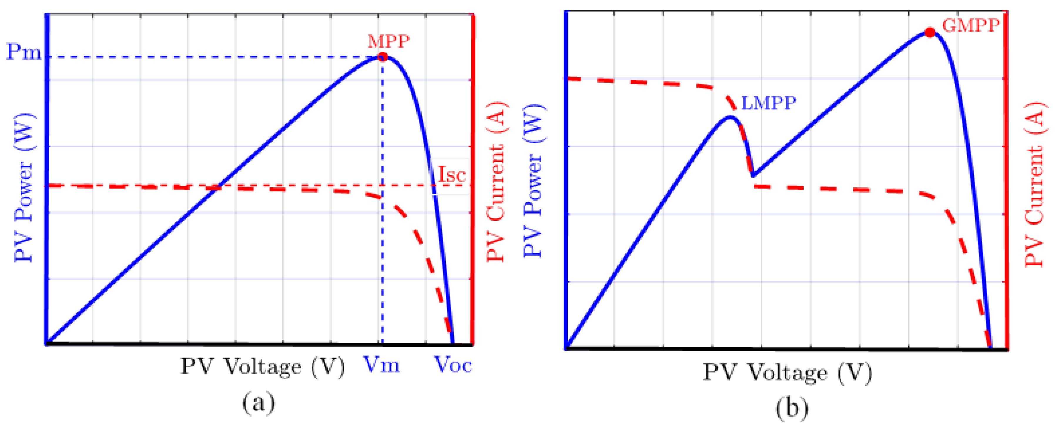
Under Uniform Irradiance (UI), all the PV modules inside the string receive the same solar irradiance and temperature. As a result, the PV modules operate effectively without damaging the modules’ cells, and the P-V curve has a single power peak on it, as shown in Figure 1a [7]. In this case, the conventional MPPT controllers can successfully reach and track that MPP. These controllersinclude Fractional Open-Circuit voltage (FOC), Fractional Short Circuit current (FSC) [8], Perturb and Observe method (P&O) [9,10], and Incremental Conductance method (IC) [11].

Under Partially Shaded Conditions (PSC), which occur when the PV string is exposed to nearby constructions, moving clouds, and adjacent trees, each PV module inside the string receives different solar irradiations and temperatures at the same time [12]. The shaded PV cells inside the module consume a certain amount of power leads to form a hotspot that causes damage for the shady locations [13]. The parallel connection of the PV module with an opposite polarity bypass diode is considered an excellent solution to the hotspot problem. On the other hand, the bypass diode affects the P-V curve characteristics by forming many power peaks [14]. These power peaks include one Global Max Power Peak (GMPP) and many other Local Power Peaks (LPPs), as shown in Figure 1b [15]. The conventional MPPT controllers may be deceived and tracked the first LMPP encountered and treated as the MPP without observing the existence of the GMPP [16].Various partial shading mitigation techniques have been introduced and classified into two significant categories named hardware-mitigation techniques and software-mitigation techniques [17].

The hardware-mitigation techniques include the use of bypass and blocking diodes [18], modification of the PV modules interconnections [19], and novel DC-DC converters [20,21]. However, they have some disadvantages, such as large size, the complexity of the interconnections, and relatively longer time for testing in laboratories.

The software mitigation techniques include stand-alone soft computing techniques or a half-breed with a conventional one. Different types of Artificial Intelligent (AI) techniques have been used [22], such as Artificial Neural Network (ANN), that require the employment of additional sensors to follow the change in climate conditions [23], Fuzzy Logic Control (FLC) that has a high complexity degree of fuzzy rules and requires previous knowledge about the system [24], and Genetic Algorithm (GA) that has a pretty high time waste for calculations which reduces the convergence speed [25]. Moreover, different types of metaheuristic algorithms have been employed for MPPT applications. Some of these algorithms are the Flower Pollination Algorithm (FPA) [26], AntColony Optimization (ACO) [27], Particle Swarm Optimization (PSO) [28], and Artificial Bee Colony (ABC). Despite these methods’ efficiency, they are challenging to implement, especially in tuning the governing equations parameters [29].

In extension to the above methods, the Cuckoo Search Algorithm (CSA) has more regular convergence, records of higher efficiency, and requires lesser tuning parameters. Despite these properties, random steps can increase the total tracking time. This paper introduced an Improved Cuckoo Search Algorithm (ICSA) for PV string MPPT under PSC, which successfully overcame the disadvantages raised by the methods of the previous discussion. This presented controller can track the GMPP under PSC without tuning parameters. It depends upon avoiding part of the exploration area after each iteration until the GMPP is captured and tracked. As a result, the GMPP is successfully tracked with minimum time spend, minimum oscillation at the transient state, and is more stable at steady state comparedwith the other methods.

To illustrate that new contribution, the Materials and Methods has been introduced in Section 2, and the Results and Discussion has been presented in Section 3. Finally, the conclusions are recorded in Section 4.

2. Materials and Methods

2.1. Modeling of Solar PV Module

Modeling of the solar PV module helps to envision its performance and predict its features under different climatic conditions.

2.1.1. Under Uniform Irradiance (UI)

In the case of UI, two PV modules are connected in series to form string-1, and each receives the same solar irradiance. The string’s PV modules are forward biased, and the same current passes through it. The bypass diodes connected in parallel with these modules are reverse biased and are virtually an open circuit, as shown in Figure 2 [29,30,31].

The PV string current-against-voltage (I-V) curve ranges from the short circuit current to zero current at the open circuit condition. The maximum output voltage is available at the open circuit condition. In addition, the maximum output current appears at the short circuit condition. The PV string’s max power point is located somewhere among these two conditions, as clarified by the P-V characteristics curve in Figure 1a [32].

The PV cell has a simulated equivalent circuit that consists of a current source, diode, series resistance, and shunt resistance, as shown in Figure 3a. During darkness, the PV cell works as a diode without producing any voltage or current. If this diode connected to an external voltage supply, it generates a current that is called the diode current ($I_D$) [33].

Applying Kirchhoff’s Current Law for the PV cell equivalent circuit, then, the mathematical equation of the PV cell output current can be represented by [33].

$$I=I_{Ph }-I_D-I_{sh}.$$

(1)

In addition,

$$I_{Ph}=\left[I_{sc}+K_i\left(T-T_r\right)\right]\times \frac{\lambda }{1000},$$

(2)

where $I_{sc}$ is the solar cell short circuit current at reference irradiance and temperature, $K_{i }$ is the short circuit current temperature coefficient, $T$ is the absolute temperature of the PV cell, $T_r$ is the reference temperature (298 Kelvin), and $\lambda$ is the solar irradiance in $(\mathrm{W}/{\mathrm{m}}^2)$ [33].

Additionally,

$$I_D=I_s\times \left[e^{\frac{q\left(\frac{V}{N_s}+\frac{I{R}_s}{N_p}\right)}{AKT}}-1\right],$$

(3)

where $I_s$ is the diode saturation current, $q$ is the electron charge $=(1.602\times {10}^{-19}\mathrm{J}/\mathrm{V})$,$N_s$ is the number of series PV cells in the module, $N_p$ is the number of parallel PV cells in the module, $A$ is the diode ideality factor, and $K$ is the Boltzmann constant $=(1.381\times {10}^{-23}\mathrm{J}/\mathrm{K})$ [34].

Moreover

$$I_s=I_{rs}\times {\left(\frac{T}{T_r}\right)}^3\times e^{\frac{q{E}_g\left(\frac{1}{T_r}-\frac{1}{T}\right)}{AK}},$$

(4)

and

$$I_{rs}=\frac{I_{sc}}{\left[e^{\frac{q{V}_{oc}}{A{N}_{s}K{T}_r}}-1\right]},$$

(5)

where $I_{rs}$ is the cell reverse saturation current, $E_g$ is the bandgap energy $=\left(1.1\mathrm{eV}\right)$, and $V_{oc}$ is the open-circuit voltage of the PV cell [34].

In addition,

$$I_{sh}=N_p\times \frac{\left(\frac{V}{N_s}+\frac{I{R}_s}{N_p}\right)}{R_{sh}},$$

(6)

where $R_{sh}$ is the internal shunt resistance of the PV cell, and $R_s$ is the internal series resistance of the PV cell.

2.1.2. Under Partial Shading Conditions (PSC)

In the case of PSC, two PV modules are connected in series to form string-2 as shown in Figure 2. One of them has a fully solar irradiance, and the other one is shaded. The shaded PV module’s short circuit current fails rapidly to zero and acts as a reverse-biased diode. The current of the non-shaded PV module causes a voltage drop across the shaded PV module. This voltage drop has a negative value and forms a hotspot on the shady location. The hotspot not only reduces the PV module efficiency but also shortens its lifetime. However, the parallel connection of the opposite polarity bypass diode prevents the shaded PV module from damage. It becomes a forward-biased diode, which allows the excess current of the non-shaded module to pass through it. This bypass operation changes the P-V’s characteristics curve by forming many power peaks on it, as shown in Figure 1b [35]. Figure 3b shows the equivalent circuit of the PV string under PSC.

2.2. CSA Idea and Its Implementation for MPPT Controller

2.2.1. The Main Idea of the CSA

The CSA is a great optimization algorithm inspired by nature and proposed by Yang and Deb in 2009 [36]. Latterly, it has been used with success in optimizing many applications and has achieved high performance. The cuckoo birds’ reproductive strategy is the basic idea that was used to construct that algorithm. To elaborate, the female cuckoo bird smartly looks for a random and fitting nest to host its eggs after it lays it. This process represents the algorithm’s searching for the optimal solution in the exploration area. There are some probabilities that the host bird may discover the strange eggs. In this case, it will either destroy them or abandon the nest and search for another one. This process represents the algorithm’s finding weak solutions and requires searching again for better solutions. The hatching and release of the production to life are the criteria for the success of the whole process. This process represents the algorithm’s finding the optimum solutions [37].

2.2.2. The CSA as a Candidate for MPPT Controller

The designers used the le’vy flight distribution equation to update the range of cuckoo’s random walking steps and stochastic shift direction during their search operation. This searching and optimization strategy can be used in solving several engineering problems, such as optimal reactive power scheduling [38], distribution network reconfiguration for power loss minimization and voltage profile improvement [39], capacitor allocations in radial distribution networks [40], and structural design optimization of vehicle components [41].

It can be also deal with the labyrinth of numerous power peaks in the PV systems’ outputs which portrayed in Figure 1b. It also helps in avoiding the slowly methods depend on scanning the P-V curve to reach and track the GMPP, as well as the possibility of processing the deception process in terms of tracking the LMPP.

Moreover, it performed quickly with minimum power oscillations. By that, the classical CSA has been successfully used in the PV systems’ MPPT controller, and the results havebeen discussed in References [28,42].

There are three bases that designers relied on to build the classical CSA algorithm. The first base is every time each one of the cuckoo birds lays one egg in a randomly chosen nest. This base is applied by the MPPT-algorithm generation of a specific number of duty cycles and sent one-by-one to the boost converter.

In the second base, the most suited nest with high-quality eggs will develop into mature birds for the next generation. This base is applied by the MPPTalgorithm’s choosing for the current best duty cycle and uses it in the next iteration.

In the third base, the number of possible nests is specified, and the number of discovered nests maintains a probability P ∈ [0, 1]. In the MPPTalgorithm, each iteration has a specific number of samples. After the evaluation process, the duty cycle corresponding to the worst power value may be rejected (destroyed) with a probability of P ∈ [0, 1]. Indemnity to that, a new duty cycle sample will be generated and evaluated to replace the rejected one. The algorithm continues to estimate until all samples reach the GMPP [37].

The steps obeyed by the CSA to track the GMPP can be normalized as follows:

Step-1: The CSA initialized (n) random samples of duty cycles and fed them one by one to the DC-DC converter.

Step-2: The PV system’s output current and voltage are measured for each duty cycle sample, and the power values are calculated and stored.

Step-3: The algorithm specifies the duty cycles (Ds) corresponding to the max power value and the min power value as the current best duty cycle sample $D_{best}$ and the worst duty cycle sample $D_{worst}$, respectively, for the current iteration.

Step-4: The algorithm tested whether the condition $\left[\mathrm{If}\left(\mathrm{rand}<P\right)\right]$ is true. If it is satisfied, the algorithm begins to replace the worst duty cycle sample with a newly generated one. Then, for the newly developed duty cycle, the PV output power is calculated, and the current best duty cycle value is updated.

Step-5: The algorithm startedto use the following le’vy flight equation to generate new $\left(n-1\right)$ duty cycle samples and fed them one-by-one to the DC-DC converter.

$$D_i^{\left(t+1\right)}=D_i^{\left(t\right)}+\alpha \oplus l{e}^{’}vy \left(\lambda \right) i=1,2,\dots ,n,$$

(7)

where

$$\alpha ={\alpha }_0\left(D_{best}-D_i\right).$$

(8)

The le’vy flight distribution equation can be simplified as

$${\alpha }_0\left(D_{best}-D_i\right)\oplus l{e}^{’}vy \left(\lambda \right)\approx k\times \left(\frac{u}{{\left|v\right|}^{1/\beta }}\right)\left(D_{best}-D_i\right),$$

(9)

where k is the le’vy multiplying coefficient, $\beta =1.5$, while $v$ and u are fined from the normal distribution curve and can be expressed as:

$$u\approx N\left(0,{\sigma }_u^2\right),v\approx N\left(0,{\sigma }_v^2\right).$$

(10)

The variables ${\sigma }_{u }^{}\mathrm{and}{\sigma }_v^{}$ can be calculated from:

$${\sigma }_{v }^{}=1,{\sigma }_{u }^{}=\left(\frac{\mathsf{\Gamma }\left(1+\beta \right)\times \sin (\mathsf{\pi }\times \beta /2)}{\mathsf{\Gamma }(\left(1+\beta \right)/2)\times \beta \times 2^{(\left(\beta -1\right)/2)}}\right),$$

(11)

where $\mathsf{\Gamma }$ is the integral gamma function [37].

Step-6: The algorithm calculates and stores the output power values for each new sample again. If all samples reach the GMPP, the algorithm stops its iteration and sends the global best duty cycle to the DC-DC converter. If not, the algorithm starts the next iteration by returning to step number three.

2.3. The Proposed Improved Cuckoo Search Algorithm (ICSA) Performance

The essential predicament in using the conventional CSA for the MPPT controller can be traced back to the size of the search steps resulting from utilizing the le’vy flight distribution equation.

During the exploration phase, the search steps contain clusters of long jumps punctuated by several short steps, as shown in Figure 4 [43].

This leads to two effective problems that are easily noticeable. First, the long jump (significant change in the duty cycle value) may lead to losing the right path towards the GMPP. It is still followed by short steps (shallow change in the duty cycle value), which lead to a verylow corresponded change in the PV module operating voltage.

Second, these steps shape may lead to research for the solution in the vicinity of a previously explored area. Thus, more iterations are required to reach the GMPP, and, during that, a bad power oscillation will transfer to the load.

Despite these, both problems can be solved by thoroughly observing the trends in several different P-V curves under uniform irradiance or partial shading conditions. From that, the proposed algorithm was designed to provide the CSA with three cumulative ideas to improve its performance in trapping and tracking the GMPP.

These ideas can be sequenced as follows:reducing the exploration area by updating its boundaries after each iteration, and replacing the worst nest (worst duty cycle sample) with another to search within the promoted site. Finally, the algorithm redirects the duty cycle samples created outside the new boundaries into the more advanced search area.

Unfortunately, there is some discrepancy in the literature on CSA. In later publications on CSA, the descriptions of the algorithm are not entirely consistent with the initial as noted by Reference [28], and discrepancies between the description and implementationsometimes exist even within the same reference, as in the case of Reference [44], The CSA described and used in this work is based on the MATLAB code similar to Reference [45]; the same version of the CSA can also be found in Reference [45].

The objective function for the CSA-based MPPT aims to maximize the PV output power by varying the duty cycle valuesthat feed one-by-one to the interface converter in the range of [0, 1]. The objective function, decision variable, and constraint can be formulated in Equations (12)–(14), respectively.

The objective function:

$$\max P_{pv}(D_i^t)=V_{pv}(D_i^t)\times I_{pv}(D_i^t).$$

(12)

The decision variable:

$$(D_i^t)=\left(\begin{array}{c}{D}_1^t\\ ⋮\\ D_n^t\end{array}\right).$$

(13)

The constraint:

$$0<D_i^t<1.$$

(14)

The proposed CSA suffices with using a population size of n = 5 (five samples of duty cycles). The values of the duty cycles limits are set to be from 0 to 1. These limits contain the real values at which the converter’s switch can be triggered.

The number of generations is differentfrom one case to other, according to the deformation of the P-V curve. So, the proposed improved CSA stops its generation when all populations (duty cycles) reach the same values (the optimum solutions), according to Equation (15).

$$P_{PV}(D_1^t)=P_{PV}(D_2^t)=P_{PV}(D_3^t)=P_{PV}(D_4^t)=P_{PV}(D_5^t).$$

(15)

2.3.1. Reduce the ExplorationArea after each Iteration

After each iteration, the proposed algorithm modified the exploration area boundaries by adding the inferred conditions listed in

Table 1. The first condition that checked by the ICSA to update the exploration area.

“Check If Condition” in Each Iteration	New Boundaries of the Exploration Area		Illustrated Design
	From	To
The right side from the reference power value
$p_C(D_i^t)>p_A(D_i^t),p_B(D_i^t)$	$v_B(D_i^t)$	$v_C(D_i^t)$
The left side from the reference power value
$p_C(D_i^t)>p_D(D_i^t),p_E(D_i^t)$	$v_C(D_i^t)$	$v_D(D_i^t)$

,

Table 2. The second condition that checked by the ICSA to update the exploration area.

“Check If Condition” in Each Iteration	New Boundaries of the Exploration Area		Illustrated Design
	From	To
The right side from the reference power value
$p_C(D_i^t)>p_A(D_i^t) \&$ $p_C(D_i^t)<p_B(D_i^t)$	$v_B(D_i^t)$	$v_C(D_i^t)$
$p_C(D_i^t)<p_A(D_i^t) \&$ $p_C(D_i^t)>p_B(D_i^t)$	$v_A(D_i^t)$
The left side from the reference power value
$p_C(D_i^t)>p_D(D_i^t) \&$ $p_C(D_i^t)<p_E(D_i^t)$	$v_C(D_i^t)$	$v_E(D_i^t)$
$p_C(D_i^t)<p_D(D_i^t) \&$ $p_C(D_i^t)>p_E(D_i^t)$		$v_D(D_i^t)$

and

Table 3. The third condition that checked by the ICSA to update the exploration area.

“Check If Condition” in Each Iteration	New Boundaries of the Exploration Area		Illustrated Design
	From	To
The right side from the reference power value
$p_C(D_i^t)<p_A(D_i^t), p_B(D_i^t)$	$v_A(D_i^t)$	$v_C(D_i^t)$
The left side from the reference power value
$p_C(D_i^t)<p_D(D_i^t), p_E(D_i^t)$	$v_C(D_i^t)$	$v_E(D_i^t)$

to the CSA performance. These conditions commutatively succeed after beginning with evenly spreading duty cycle samples ($D_1^1=0.1$, ${\mathrm{D}}_2^1=0.3$, $D_3^1=0.5$, $D_4^1=0.7$, $D_5^1=0.9$) to cover the entire P-V curve in the first iteration, as shown in Figure 5a.

Then, iteratively, the duty cycles $(D_i^t)$, voltages $(V_i^t)$, and powers $(P_i^t)$ values are stored in a $3\times 3$ matrix, in descending order, according to the iteration’s operating voltage values. The matrix rows are marked by the characters (A, B, C, D, and E), as shown in Figure 5b.

The upper and lower subscript for the duty cycle $(D_i^t)$ indicates the number of iteration and the sample number, respectively.

Now, the arranged voltage values achieve:

$$v_A(D_i^t)>v_B(D_i^t)>v_C(D_i^t)>v_D(D_i^t)>v_E(D_i^t).$$

(16)

The operating voltage $v_C(D_i^t)$ stored in the matrix’s row “C” is the middle voltage value located on the P-V curve. Its corresponding power value $p_C(D_i^t)$ is considered the reference power value for the present iteration, as shown in Figure 5.

The reference power value divides the exploration area into two asymmetric regions. The boundaries of each region are decreased towards the optimum solution after each iteration. These decreasedoperations can be achieved by checking the relationship between the reference power value and the other iteration’s power values. This relationship can be classified into three main conditions.

In the first condition, where the reference power value is the highest, the probability of finding GMPP around the reference power region is higher than that of the surrounding region around the lesser other powers’ values.

From that, the proposed algorithm neglects the area in which the GMPP is unlikely to be found and sets the voltage $v_B(D_i^t)$ or $v_D(D_i^t)$ to be the new exploration area limit, as described in Table 1.

In the second condition, the reference power value is neither the highest nor the lowest power values in that iteration. In this case, the proposed algorithm promotes the area between the reference power value and the highest power value for the next search operation, as described in Table 2.

In the third condition, the value of the reference power is the lowest. The proposed algorithm repeats the search inside the allsearch area, as described in Table 3.

2.3.2. Replace the Worst Nest (Worst Duty Cycle Sample) with the Better One

During the procedure of the proposed method, the algorithm stores the highest two power values and their corresponding duty cycles $D\left(P_{max1}\right)$ and $D\left(P_{max2}\right)$. These values can be used to complete the algorithm performance and prevent the dismissal of the exploration area that contains the optimum solution. After each iteration, the algorithm replaces the worst solution (discovered nest) with another duty cycle value, mediating the distance between the two highest power values, and calculated by Equation (17), as shown in Figure 6.

$$D_{New}=D\left(P_{max2}\right)+\frac{D\left(P_{max1}\right)-D\left(P_{max2}\right)}{2}.$$

(17)

2.3.3. Redirect the Samples Created outside the New Exploration Area’s Boundaries

Iteratively, the duty cycles $D\left(P_{max1}\right)$ and $D\left(P_{max2}\right)$ are updated, and the ICSA begins to generate new samples of duty cycles by using Equation (7). If any duty cycle sample is generated outside the boundaries of the new exploration area, the algorithm replaces that sample with another one that mediates the values of the fitnessduty cycles $D\left(P_{max1}\right)$ and $D\left(P_{max2}\right)$ by using Equation (17), as shown in Figure 6.

The flowchart of the proposed technique can be simplified, as in Figure 7.

3. The Results and Discussion

3.1. The Simulation Results

In this section, the proposed ICSA is implemented using MATLAB/Simulink software. This simulation software has been used to compare the transient and the steady-state performance between both the ICSA and classical one.

The PV string simulation pattern is consisting of a number of PV modules. Each one has a shunt connection with a bypass diode. The multitude of the peaks and their positions on the P-V curve can be controlled using different irradiance values at the same surrounding temperature. The PV module and the boost converter parameters are listed in

Table 4. The simulation system’s parameters.

The Parameters of the PV Module	Values	The Parameters of the Boost Converter	Values
Short circuit current $I_{sc}$	8.02 A	The input capacitor $C_{in}$	10 µF
Open circuit voltage $V_o$	21.9 V	The converter inductor $L$	1.1 mH
Voltage at max power point $V_m$	17.6 V	The switch frequency $f$	50 kHz
Current at max power point $I_m$	7.39 A	The output capacitor $C_{out}$	0.5 mF

. The simulation was studied and performed under uniform irradiance and PSC.

3.1.1. Under Uniform Irradiance Case

In this case, pattern-1 is a PV string consisting of two PV modules, and each received the same irradiance level equals to $1000\mathrm{W}/{\mathrm{m}}^2.$ So, the string’s P-V curve has one power peak of $260 \mathrm{W}.$ The duty cycles’ operating points for the first four iterations are shown in Figure 8a, and its data are listed in

Table 5. The rearranged and saved data for pattern-1.

Matrix Row	The First Iteration Matrix				The Second Iteration Matrix				The Third Iteration Matrix				The Fourth Iteration Matrix
	n	D	VPV (V)	PPV (W)	n	D	VPV (V)	PPV (W)	n	D	VPV (V)	PPV (W)	n	D	VPV (V)	PPV (W)
$A$	$D_1^1$	0.1	43.20	36.5	$D_1^2$	0.3481	42.54	72.13	$D_1^3$	0.6082	39.78	195.7	$D_2^4$	0.6167	39.54	203.7
$B$	$D_2^1$	0.3	42.71	67.2	$D_4^2$	0.5114	41.17	142.3	$D_3^3$	0.6025	39.86	192.9	$D_3^4$	0.6260	39.30	208.8
$C$	$D_3^1$	0.5	41.50	126.3	$D_2^2$	0.6005	39.42	206.3	$D_2^3$	0.6255	39.24	211.2	$D_4^4$	0.6475	38.65	226.2
$D$	$D_4^1$	0.7	29.78	231.7	$D_3^2$	0.6544	37.67	243.5	$D_5^3$	0.6322	39.16	213.6	$D_5^4$	0.6726	37.08	250.7
$E$	$D_5^1$	0.9	7.88	62.77	$D_5^2$	0.7	29.75	231.7	$D_4^3$	0.6544	37.84	240.9	$D_1^4$	0.6908	34.86	258.7
True condition	$p_C(D_3^1)>p_A(D_1^1) \&p_C(D_3^1)>p_B(D_2^1)$ $p_C(D_3^1)<p_D(D_4^1) \& p_C(D_3^1)>p_E(D_5^1)$				$p_C(D_2^2)>p_A(D_1^2) \&p_C(D_2^2)>p_B(D_4^2)$ $p_C(D_2^2)<p_D(D_3^2) \&p_C(D_2^2)<p_E(D_5^2)$				$p_C(D_2^3)>p_A(D_1^3) \&p_C(D_2^3)>p_B(D_3^3)$ $p_C(D_2^3)<p_D(D_5^3) \&p_C(D_2^3)<p_E(D_4^3)$				$p_C(D_4^4)>p_A(D_2^4) \&p_C(D_4^4)>p_B(D_3^4)$ $p_C(D_4^4)<p_D(D_5^4) \&p_C(D_4^4)<p_E(D_1^4)$
New boundaries	$from v_B\left(D_2^1\right) to v_D\left(D_4^1\right)$				$from v_B\left(D_4^2\right)to v_E\left(D_5^2\right)$				$from v_B\left(D_3^3\right) to v_E\left(D_4^3\right)$				$from v_B\left(D_3^4\right) to v_E\left(D_1^4\right)$

. Table 5 also identifies the true conditions recommended by the ICSA, through which it outlines the exploration area boundaries for the next iteration. In the third iteration, the MPP is located outside the new exploration boundaries. However, the proposed algorithm usually returns searched inside the region between the two highest power values has been reached before, as discussed in the previous section. Consequently, in the fourth iteration, the MPP returns inside the new boundaries of the exploration area.

The duty cycles convergence towards the MPP for each CSA and the ICSA are shown in Figure 8b,c, respectively. It can be observed that the performance of the ICSA leads to track the MPP of $260 \mathrm{W}$ in about 0.5 s, while the classical CSA takes 0.8 s, with bad fluctuations.

3.1.2. Under PSC Case

In the First Case

Pattern-2 is a PV string consisting of three PV modules, and each received different irradiance levels equals to $1000\mathrm{W}/{\mathrm{m}}^2,1000\mathrm{W}/{\mathrm{m}}^2,$ and $400\mathrm{W}/{\mathrm{m}}^2.$ So, the P-V curve of the PV string has two power peaks equals $254 \mathrm{W},$ and $177 \mathrm{W}$. The duty cycles’ operating points for the first four iterations are displayed in Figure 9a, and its data are arranged in

Table 6. The rearranged and saved data for pattern-2.

Matrix Row	The First Iteration Matrix				The Second Iteration Matrix				The Third Iteration Matrix				The Fourth Iteration Matrix
	n	D	VPV (V)	PPV (W)	n	D	VPV (V)	PPV (W)	n	D	VPV (V)	PPV (W)	n	D	VPV (V)	PPV (W)
$A$	$D_1^1$	0.1	63.14	81.52	$D_4^2$	0.5114	47.92	151.8	$D_1^3$	0.5	49.37	155.8	$D_2^4$	0.5371	44.83	143
$B$	$D_2^1$	0.3	60.51	160	$D_2^2$	0.5303	42.99	137.7	$D_5^3$	0.5547	44.23	141.2	$D_3^4$	0.5934	39.43	176.4
$C$	$D_3^1$	0.5	43	137	$D_1^2$	0.5	41.61	133.7	$D_3^3$	0.6670	37.22	233.1	$D_5^4$	0.7	34.34	253
$D$	$D_4^1$	0.7	30.11	233.3	$D_3^2$	0.6544	36.69	240.6	$D_4^3$	0.6742	36.71	240.3	$D_4^4$	0.7	33.62	251.8
$E$	$D_5^1$	0.9	8.2	64.39	$D_5^2$	0.7	32.04	245.4	$D_2^3$	0.6657	36.31	244.8	$D_1^4$	0.7	32.22	246.3
True condition	$p_C(D_3^1)>p_A(D_1^1) \&p_C(D_3^1)<p_B(D_2^1)$ $p_C(D_3^1)<p_D(D_4^1) \& p_C(D_3^1)>p_E(D_5^1)$				$p_C(D_1^2)<p_A(D_4^2) \&p_C(D_1^2)<p_B(D_2^2)$ $p_C(D_1^2)<p_D(D_3^2) \&p_C(D_1^2)<p_E(D_5^2)$				$p_C(D_3^3)>p_A(D_1^3) \&p_C(D_3^3)>p_B(D_5^3)$ $p_C(D_3^3)<p_D(D_4^3) \&p_C(D_3^3)<p_E(D_2^3)$				$p_C(D_5^4)>p_A(D_2^4) \&p_C(D_5^4)>p_B(D_3^4)$ $p_C(D_5^4)>p_D(D_4^4) \& p_C(D_5^4)>p_E(D_1^4)$
New boundaries	$from v_B\left(D_2^1\right) to v_D\left(D_4^1\right)$				$from v_A\left(D_4^2\right) to v_E\left(D_5^2\right)$				$from v_B\left(D_5^3\right) to v_E\left(D_2^3\right)$				$from v_B\left(D_3^4\right) to v_D\left(D_4^4\right)$

. Table 6 also identifies the true conditions approved by the ICSA, through which it outlines the exploration area boundaries for the next iteration. The duty cycle convergence towards the GMPP for each CSA and the ICSA are shown in Figure 9b,c, respectively. It can be observed that the performance of the ICSA leads to track the GMPP of $254 \mathrm{W}$ in about 0.5 s, while the classical CSA takes 0.87 s, with disagreeable oscillations.

In the Second Case

Pattern-3 is a PV string consisting of four PV modules, and each received different irradiance levels equals to $1000\mathrm{W}/{\mathrm{m}}^2,1000\mathrm{W}/{\mathrm{m}}^2,500\mathrm{W}/{\mathrm{m}}^2,$ and $200\mathrm{W}/{\mathrm{m}}^2.$ So, the P-V curve of the PV string has three power peaks equals $247\mathrm{W},217\mathrm{W},$ and $119\mathrm{W}$. The duty cycles’ operating points for the first four iterations are exhibited in Figure 10a, and its data are scheduled in

Table 7. The rearranged and saved data for pattern-3.

Matrix Row	The First Iteration Matrix				The Second Iteration Matrix				The Third Iteration Matrix				The Fourth Iteration Matrix
	n	D	VPV (V)	PPV (W)	n	D	VPV (V)	PPV (W)	n	D	VPV (V)	PPV (W)	n	D	VPV (V)	PPV (W)
$A$	$D_1^1$	0.1	64.04	102.7	$D_4^2$	0.5114	51.17	200.7	$D_3^3$	0.5366	49.33	194.2	$D_3^4$	0.5934	41.63	166.5
$B$	$D_2^1$	0.3	61.19	143.1	$D_2^2$	0.5303	48.59	191.6	$D_5^3$	0.5547	46.27	183.3	$D_4^4$	0.5906	41.26	165.1
$C$	$D_3^1$	0.5	47.13	186.4	$D_1^2$	0.6	38.50	176.9	$D_1^3$	0.6	40.33	161.8	$D_2^4$	0.6836	35.39	240.4
$D$	$D_4^1$	0.7	31.42	240.2	$D_3^2$	0.6544	36.88	220.5	$D_4^3$	0.6742	35.81	236.2	$D_1^4$	0.7	32.88	246
$E$	$D_5^1$	0.9	8.39	66.7	$D_5^2$	0.7	33.03	246.4	$D_2^3$	0.6798	34.83	244.2	$D_5^4$	0.7	32.44	244.7
True condition	$p_C(D_3^1)>p_A(D_1^1) \&p_C(D_3^1)>p_B(D_2^1)$ $p_C(D_3^1)<p_D(D_4^1) \& p_C(D_3^1)>p_E(D_5^1)$				$p_C(D_1^2)<p_A(D_4^2) \&p_C(D_1^2)<p_B(D_2^2)$ $p_C(D_1^2)<p_D(D_3^2) \&p_C(D_1^2)<p_E(D_5^2)$				$p_C(D_1^3)<p_A(D_3^3) \&p_C(D_1^3)<p_B(D_5^3)$ $p_C(D_1^3)<p_D(D_4^3) \&p_C(D_1^3)<p_E(D_2^3)$				$p_C(D_2^4)>p_A(D_3^4) \&p_C(D_2^4)>p_B(D_4^4)$ $p_C(D_2^4)<p_D(D_1^4) \&p_C(D_2^4)<p_E(D_5^4)$
New boundaries	$from v_B\left(D_2^1\right) to v_D\left(D_4^1\right)$				$from v_A\left(D_4^2\right) to v_E\left(D_5^2\right)$				$from v_A\left(D_3^3\right) to v_E\left(D_2^3\right)$				$from v_B\left(D_4^4\right) to v_E\left(D_5^4\right)$

. Table 7 also identifies the true conditions commended by the ICSA, through which it outlines the exploration area boundaries for the next iteration. The duty cycle convergence towards the GMPP for each CSA and the ICSA are shown in Figure 10b,c, respectively. It can be observed that the performance of the ICSA leads to track the GMPP of $247\mathrm{W}$ in about 0.4 s, while the classical CSA takes 0.8 s, with disturbing fluctuations.

In the Third Case

Pattern-4 is a PV string consisting of four PV modules, and each received different irradiance levels equals $1000\mathrm{W}/{\mathrm{m}}^2,700\mathrm{W}/{\mathrm{m}}^2,500\mathrm{W}/{\mathrm{m}}^2,$ and $300\mathrm{W}/{\mathrm{m}}^2.$ So, the P-V curve of the PV string has four power peaks equals 111 W, 186 W, 210 W, and 178 W. The duty cycles’ operating points for the first four iterations are presented in Figure 11a, and its data are entered in

Table 8. The rearranged and saved data for pattern-4.

Matrix Row	The First Iteration Matrix				The Second Iteration Matrix				The Third Iteration Matrix				The Fourth Iteration Matrix
	n	D	VPV (V)	PPV (W)	n	D	VPV (V)	PPV (W)	n	D	VPV (V)	PPV (W)	n	D	VPV (V)	PPV (W)
$A$	$D_1^1$	0.1	65.58	149.3	$D_1^2$	0.3	60.9	137.6	$D_3^3$	0.3902	59.38	166	$D_5^4$	0.4792	55.23	199.9
$B$	$D_2^1$	0.3	60.94	137.24	$D_2^2$	0.3869	59.43	165.6	$D_4^3$	0.4772	53.08	194	$D_4^4$	0.4818	54.84	199.3
$C$	$D_3^1$	0.5	47.03	175.72	$D_3^2$	0.4772	52.95	194.7	$D_5^3$	0.4948	51.92	191	$D_3^4$	0.4819	54.56	198.7
$D$	$D_4^1$	0.7	27.46	146.85	$D_4^2$	0.5	51.13	188.8	$D_2^3$	0.4886	50.89	187.98	$D_2^4$	0.4865	53.73	196
$E$	$D_5^1$	0.9	7.26	56.59	$D_5^2$	0.524	48.17	179.2	$D_1^3$	0.5918	39.08	149	$D_1^4$	0.4886	35.1	194
True condition	$p_C(D_3^1)>p_A(D_1^1) \&p_C(D_3^1)>p_B(D_2^1)$ $p_C(D_3^1)>p_D(D_4^1) \& p_C(D_3^1)>p_E(D_5^1)$				$p_C(D_3^2)>p_A(D_1^2) \&p_C(D_3^2)>p_B(D_2^2)$ $p_C(D_3^2)>p_D(D_4^2) \& p_C(D_3^2)>p_E(D_5^2)$				$p_C(D_5^3)>p_A(D_3^3) \&p_C(D_5^3)<p_B(D_4^3)$ $p_C(D_5^3)>p_D(D_2^3) \& p_C(D_5^3)>p_E(D_1^3)$				$p_C(D_3^4)<p_A(D_5^4) \&p_C(D_3^4)<p_B(D_4^4)$ $p_C(D_3^4)>p_D(D_2^4) \& p_C(D_3^4)>p_E(D_1^4)$
New boundaries	$from v_B\left(D_2^1\right) to v_D\left(D_4^1\right)$				$from v_B\left(D_2^2\right) to v_D\left(D_4^2\right)$				$from v_B\left(D_4^3\right) to v_D\left(D_2^3\right)$				$from v_A\left(D_5^4\right) to v_D\left(D_2^4\right)$

. Table 8 also identifies the true conditions sanctioned by the ICSA, through which it outlines the exploration area boundaries for the next iteration. The duty cycle convergence towards the GMPP for each CSA and the ICSA are shown in Figure 11b,c, respectively. It can be observed that the performance of the ICSA leads to track the GMPP of $210\mathrm{W}$ in about 0.25 s, while the classical CSA takes 0.8 s, with unfortunate fluctuations.

3.2. The Experimental Results

The effectiveness of the proposed ICSA is verified by an empirical test in the laboratory, as shown in Figure 12a. The experimental setup has three main parts. The first part is the PV emulator circuit, which consists of two variable DC power supplies and several power resistances. The second part is the interface device is represented by a boost converter that has the inductor of “3 mH, 7 A”, capacitor of “2 × 2200 μF, 50 V”, fast recovery diode of “100 V, 10 A”, and power MOSFET of “100 V, 25 A”. The final part is the controllerconsists of a current sensor, voltage sensor, gate drive, and a “TMS320F28335”microcontroller with 32-bits, 150 MHz. The experimental output is joined to a battery load of “2 × 12 V, 7 Ah”.

3.2.1. Uniform Irradiance Condition

The suggested ICSA was appraised and compared with the performance of the classical CSA and the P&O method under uniform irradiance conditions. This case can be simulated by setting the two DC power supplies to 15 V and using two power resistances equals 3.3 Ω. Hence, the output nonlinear P-V curve has a single peak at 64 W. The experiment outputs for voltage, current, and power values are measured and portrayed by using an oscilloscope, as shown in Figure 13.

It was clearly seen that the P&O method reached the MPP at 64.5 W in about 0.5 s, but it has a high oscillation in both the transient and the steady-state conditions, as shown in Figure 13a,b, respectively. The classical CSA took a long time of 1.2 s to converged and reach the MPP, as shown in Figure 13c. Then, it catches and tracks the MPP of 59.9 W at the steady-state conditions, as demonstrated in Figure 13d. On the other hand, the ICSA takes less than 0.5 s to get the MPP, as shown in Figure 13e. After that, it transfers about 63.8 W to the load with high power stability in steady-state conditions, as shown in Figure 13f. From this test, the results indicate that the proposed ICSA has a quicker performance speed with higher stability than the other two methods.

3.2.2. PSC

In this case study, the two DC power supplies are set to 20 V and use two power resistance equals 2 Ω and 8.5 Ω, as shown in Figure 12b. The simulated PV output has two MPPs of 45 W and 37 W. The same previous algorithms are re-evaluated to determine the most efficient under partially shaded conditions.

If the P&O explorer does not fall into the LMPP and catches the GMPP, the step size remains very influential on the shape of the output transmitted to the load. In adjusting the step size by 0.0001, the search will be prolonged and reach the power of 42.6 W, as shown in Figure 14a. In contrast, if the step size is set to 0.1, the algorithm reaches a power value of 45.3 W but with an annoying vibration around the GMPP, as shown in Figure 14b.

The classical CSA converged to the GMPP in about 0.68 s and transferred 44.1 W to the load at steady-state conditions, as shown in Figure 14c,d, respectively. On the other hand, the ICSA reached the GMPP at about 0.08 s with high stability output power of 45.4 W, as shown in Figure 14e,f, respectively.

From this test, the results indicate that the proposed ICSA has a shorter time to track the GMPP with higher stability than the other two methods.

4. Conclusions

Theproposed technique presented in this article adds an effective mechanism to the classical Cuckoo Search Algorithm performance to improve the PV systems’ Global Max Power Point Tracking. This mechanism updates the boundaries of the exploration area after each iteration by promotingthe exploration area containing the high-quality solutions and excludingthe exploration area containing the poor solutions. The simulation results showed the performance of the proposed technique in the first four iterations, as well as the waveform trajectory towards the GMPP, for several different models. On the other hand, an experimental setup compared the performance of the proposed technique with both the classical CSA and the P&O method. The results indicate that the proposed technique has a minimum tracking time with high output power stability at the steady-state condition, especially at the partial shading conditions.

The proposed CSA offers a better response than the classical one for both the settling time and output oscillations. These achievements are mainly due to the novel proposed scan period sectionalizing. The fear from misconvergence in the investigated optimization problem is of less importance in this case. The core of the proposed technique relies on the fact that reducing the exploration area is based on maximizing the overall PV string power, continuously taking into consideration the dynamic array voltage variation and avoiding less probability search areas, hence avoiding the misconvergence. It is better to declare that this benefit is application specific and needs better knowledge of the investigated problem practical dynamics. Hence, the authors cannot guarantee its applicability for different applications unless deeply investigated.

References

1. De Brito, M.A.G.; Galotto, L.; Sampaio, L.P.; e Melo, G.D.A.; Canesin, C.A. Evaluation of the main MPPT techniques for photovoltaic applications. IEEE Trans. Ind. Electron. 2012, 60, 1156–1167. [Google Scholar] [CrossRef]
2. Kollimalla, S.K.; Mishra, M.K. Novel adaptive P&O MPPT algorithm for photovoltaic sys-tem considering sudden changes in weather condition. In Proceedings of the International Conference on Clean Electrical Power (ICCEP), Alghero, Italy, 11–13 June 2013; pp. 653–658. [Google Scholar]
3. Xiao, W.; Lind, M.G.J.; Dunford, W.G.; Capel, A. Real-Time Identification of Optimal Operating Points in Photovoltaic Power Systems. IEEE Trans. Ind. Electron. 2006, 53, 1017–1026. [Google Scholar] [CrossRef]
4. Razali, N.M.; Rahim, N. DSP-based maximum peak power tracker using P&O algorithm. In Proceedings of the 2011 IEEE Conference on Clean Energy and Technology (CET), Kuala Lumpur, Malaysia, 27–29 June 2011; pp. 34–39. [Google Scholar] [CrossRef]
5. Nugraha, S.D.; Qudsi, O.A.; Yanaratri, D.S.; Sunarno, E.; Sudiharto, I. MPPT-current fed push pull converter for DC bus source on solar home application. In Proceedings of the 2017 2nd International conferences on Information Technology, Information Systems and Electrical Engineering (ICITISEE), Yogyakarta, Indonesia, 1–2 November 2017; pp. 378–383. [Google Scholar] [CrossRef]
6. Chowdhury AS, K.; Razzak, M.A. Single phase grid-connected photovoltaic inverter for residential application with maximum power point tracking. In Proceedings of the 2013 International Conference on Informatics, Electronics and Vision (ICIEV), Dhaka, Bangladesh, 17–18 May 2013. [Google Scholar]
7. Ahmed, J.; Salam, Z. An accurate method for MPPT to detect the partial shading occurrence in a PV system. IEEE Trans. Ind. Inform. 2017, 13, 2151–2161. [Google Scholar] [CrossRef]
8. Al-Soeidat, M.R.; Cembrano, A.; Lu, D.D.-C. Comparing effectiveness of hybrid mppt algorithms under partial shading conditions. In Proceedings of the 2016 IEEE International Conference on Power System Technology (POWERCON), Wollongong, Australia, 28 September–1 October 2016; pp. 1–6. [Google Scholar] [CrossRef] [Green Version]
9. Abdelsalam, A.K.; Massoud, A.M.; Ahmed, S.; Enjeti, P.N. High-Performance Adaptive Perturb and Observe MPPT Technique for Photovoltaic-Based Microgrids. IEEE Trans. Power Electron. 2011, 26, 1010–1021. [Google Scholar] [CrossRef]
10. Ahmed, J.; Salam, Z. An enhanced adaptive P&O MPPT for fast and efficient tracking under varying environmental conditions. IEEE Trans. Sustain. Energy 2018, 9, 1487–1496. [Google Scholar]
11. Tey, K.S.; Mekhilef, S. Modified incremental conductance algorithm for photovoltaic system under partial shading conditions and load variation. IEEE Trans. Ind. Electron. 2014, 61, 5384–5392. [Google Scholar]
12. Ahmad, J.; Spertino, F.; Di Leo, P.; Ciocia, A. A module voltage based maximum power point tracking algo-rithm for photovoltaic arrays under partial shading conditions. In Proceedings of the 57th International Scientific Conference on Power and Electrical Engineering of Riga Technical University (RTUCON), Riga, Latvia, 13–14 October 2016; pp. 1–6. [Google Scholar]
13. Darussalam, R.; Pramana, R.I.; Rajani, A. Experimental investigation of serial parallel and total-cross-tied configuration photovoltaic under partial shading conditions. In Proceedings of the International Conference on Sustainable Energy Engineering and Application (ICSEEA), Jakarta, Indonesia, 23–24 October 2017; pp. 140–144. [Google Scholar]
14. Mahmoud, Y.; El-Saadany, E.F. Fast Power-Peaks Estimator for Partially Shaded PV Systems. IEEE Trans. Energy Convers. 2015, 31, 206–217. [Google Scholar] [CrossRef]
15. Gosumbonggot, J.; Fujita, G. Partial Shading Detection and Global Maximum Power Point Tracking Algorithm for Photovoltaic with the Variation of Irradiation and Temperature. Energies 2019, 12, 202. [Google Scholar] [CrossRef] [Green Version]
16. Huynh, D.C.; Nguyen, T.M.; Dunnigan, M.W.; Mueller, M.A. Global MPPT of solar PV modules using a dynamic PSO algorithm under partial shading conditions. In Proceedings of the 2013 IEEE Conference on Clean Energy and Technology (CEAT), Langkawi, Malaysia, 18–20 November 2013; pp. 134–139. [Google Scholar] [CrossRef]
17. Salam, Z.; Ramli, Z.; Ahmed, J.; Amjad, M. Partial shading in building integrated PV system: Causes, effects and mitigating techniques. Int. J. Power Electron. Drive Syst. 2015, 6, 712–722. [Google Scholar] [CrossRef]
18. Eltamaly, A.M.; Abdelaziz, A.Y. (Eds.) Modern Maximum Power Point Tracking Techniques for Photovoltaic Energy Systems; Springer: Berlin/Heidelberg, Germany, 2019. [Google Scholar]
19. Sahu, H.S.; Nayak, S.K. Extraction of Maximum Power from a PV Array under Nonuniform Irradiation Conditions. IEEE Trans. Electron. Devices 2016, 63, 4825–4831. [Google Scholar] [CrossRef]
20. Abolhasani, M.A.; Rezaii, R.; Beiranvand, R.; Varjani, A.Y. A comparison between buck and boost topologies as module integrated converters to mitigate partial shading effects on PV arrays. In Proceedings of the 2016 7th Power Electronics and Drive Systems Technologies Conference (PEDSTC), Tehran, Iran, 16–18 February 2016; pp. 367–372. [Google Scholar] [CrossRef]
21. Rezaii, R.; Abolhasani, M.A.; Varjani, A.Y.; Beiranvand, R. Analysis of the boost converter under the DCM condition to reduce the MIC volume to mitigate partial shading effects in PV arrays. In Proceedings of the 2016 7th Power Electronics and Drive Systems Technologies Conference (PEDSTC), Tehran, Iran, 16–18 February 2016; pp. 349–355. [Google Scholar]
22. Alshareef, M.; Lin, Z.; Ma, M.; Cao, W. Accelerated Particle Swarm Optimization for Photovoltaic Maximum Power Point Tracking under Partial Shading Conditions. Energies 2019, 12, 623. [Google Scholar] [CrossRef] [Green Version]
23. Elobaid, L.M.; Abdelsalam, A.K.; Zakzouk, E.E. Artificial neural network-based photovoltaic maximum power point tracking techniques: A survey. IET Renew. Power Gener. 2015, 9, 1043–1063. [Google Scholar] [CrossRef]
24. Hong, Y.-Y.; Buay, P.M.P.; Beltran, A.A. Maximum Power Point Tracking of Photovoltaic System Using Taguchi-based Fuzzy Logic Control. In Proceedings of the 2019 IEEE Milan PowerTech, Milan, Italy, 23–27 June 2019; pp. 1–6. [Google Scholar] [CrossRef]
25. Smida, M.B.; Sakly, A. Genetic based algorithm for maximum power point tracking (MPPT) for grid connected PV systems operating under partial shaded conditions. In Proceedings of the 7th International Conference on Modelling, Identification and Control (ICMIC), Sousse, Tunisia, 18–20 December 2015; pp. 1–6. [Google Scholar]
26. Ram, J.P.; Rajasekar, N. A novel flower pollination based global maximum power point method for solar maximum power point tracking. IEEE Trans. Power Electron. 2016, 32, 8486–8499. [Google Scholar]
27. Jiang, L.L.; Maskell, D.L.; Patra, J. A novel ant colony optimization-based maximum power point tracking for photovoltaic systems under partially shaded conditions. Energy Build. 2013, 58, 227–236. [Google Scholar] [CrossRef]
28. Ahmed, J.; Salam, Z. A Maximum Power Point Tracking (MPPT) for PV system using Cuckoo Search with partial shading capability. Appl. Energy 2014, 119, 118–130. [Google Scholar] [CrossRef]
29. Soualmia, A.; Chenni, R. A survey of maximum peak power tracking techniques used in photovoltaic power systems. In Proceedings of the 2016 Future Technologies Conference (FTC), San Francisco, CA, USA, 6–7 December 2016; pp. 430–443. [Google Scholar] [CrossRef]
30. Higashitani, M.; Ishigame, A.; Yasuda, K. Particle Swarm Optimization Considering the Concept of Predator-Prey Behavior. In Proceedings of the 2006 IEEE International Conference on Evolutionary Computation, Vancouver, BC, Canada, 16–21 July 2006; pp. 434–437. [Google Scholar] [CrossRef]
31. Winston, D.P.; Kumar, B.P.; Christabel, S.C.; Chamkha, A.J.; Sathyamurthy, R. Maximum power extraction in solar renewable power system—A bypass diode scanning approach. Comput. Electr. Eng. 2018, 70, 122–136. [Google Scholar] [CrossRef]
32. Babu, B.C.; Cermak, T.; Gurjar, S.; Leonowicz, Z.M.; Piegari, L. Analysis of mathematical modeling of PV module with MPPT algorithm. In Proceedings of the 2015 IEEE 15th International Conference on Environment and Electrical Engineering (EEEIC), Rome, Italy, 10–13 June 2015; pp. 1625–1630. [Google Scholar]
33. Windarko, N.A.; NizarHabibi, M.; Sumantri, B.; Prasetyono, E.; Efendi, M.Z.; Taufik. A New MPPT Algorithm for Photovoltaic Power Generation under Uniform and Partial Shading Conditions. Energies 2021, 14, 483. [Google Scholar] [CrossRef]
34. Mohammed, S.S. Modeling and Simulation of Photovoltaic module using MATLAB/Simulink. Int. J. Chem. Environ. Eng. 2011, 2, 350–355. [Google Scholar]
35. Varshney, S.K.; Khan, Z.A.; Husain, M.A.; Tariq, A. A comparative study and investigation of different diode models incorporating the partial shading effects. In Proceedings of the 2016 International Conference on Electrical, Electronics, and Optimization Techniques (ICEEOT), Chennai, India, 3–5 March 2016; pp. 3145–3150. [Google Scholar] [CrossRef]
36. Nugraha, D.A.; Lian, K.L. A novel MPPT method based on cuckoo search algorithm and golden section search algorithm for partially shaded PV system. Can. J. Electr. Comput. Eng. 2019, 42, 173–182. [Google Scholar] [CrossRef]
37. Eltamaly, A. An Improved Cuckoo Search Algorithm for Maximum Power Point Tracking of Photovoltaic Systems under Partial Shading Conditions. Energies 2021, 14, 953. [Google Scholar] [CrossRef]
38. Reddy, S.S. Optimal Reactive Power Scheduling Using Cuckoo Search Algorithm. Int. J. Electr. Comput. Eng. 2017, 7, 2349. [Google Scholar]
39. Nguyen, T.T.; Truong, A.V. Distribution network reconfiguration for power loss minimization and voltage profile improvement using cuckoo search algorithm. Int. J. Electr. Power Energy Syst. 2015, 68, 233–242. [Google Scholar] [CrossRef]
40. El-Fergany, A.A.; Abdelaziz, A.Y. Capacitor allocations in radial distribution networks using cuckoo search algorithm. IET Gener. Transm. Distrib. 2014, 8, 223–232. [Google Scholar] [CrossRef] [Green Version]
41. Durgun, İ.; Yildiz, A.R. Structural design optimization of vehicle components using cuckoo search algorithm. Mater. Test. 2012, 54, 185–188. [Google Scholar] [CrossRef]
42. Ahmed, J.; Salam, Z. A soft computing MPPT for PV system based on Cuckoo Search algorithm. In Proceedings of the 4th International Conference on Power Engineering, Energy and Electrical Drives, Istanbul, Turkey, 13–17 May 2013; pp. 558–562. [Google Scholar] [CrossRef]
43. Wen, X.Y.; Lin, P.J.; Chen, Z.C.; Wu, L.J.; Cheng, S.Y. A grid-connected single-phase photovoltaic micro inverter. In IOP Conference Series: Earth and Environmental Science; IOP Publishing: Bristol, UK, 2017; p. 012079. [Google Scholar]
44. Yang, X.S. Nature-Inspired Optimization Algorithms; Elsevier: Amsterdam, The Netherlands, 2014; pp. 1–263. [Google Scholar]
45. Yang, X.S. Cuckoo Search (CS) Algorithm Version 1.3. MATLAB Central File Exchange. 2013. Available online: https://se.mathworks.com/matlabcentral/fileexchange/29809-cuckoo-search--cs--algorithm (accessed on 28 October 2017).
Figure 1. The PV string’s P-V and I-V curves: (a) under (UI); (b) under (PSC).
Energies 14 07210 g001
Figure 2. Model of the PV stringstructure.
Energies 14 07210 g002
Figure 3. The equivalent circuit of the PV cells: (a) under (UI); (b) under (PSC).
Energies 14 07210 g003
Figure 4. The le’vy flight works in a 2D plane.
Energies 14 07210 g004
Figure 5. (a) The spread of the iteration’s operating points on the P-V curve. (b) The iteration’s data storage matrix.
Energies 14 07210 g005
Figure 6. The new position of the weakened duty cycles towards the GMPP.
Energies 14 07210 g006
Figure 7. The flowchart of the proposed (ICSA).
Energies 14 07210 g007
Figure 8. The MPP tracking method for pattern-1. (a) The samples’ operating points at the first four iterations. (b) The tracking performance by using CSA. (c) The tracking performance by using ICSA.
Energies 14 07210 g008
Figure 9. The GMPP tracking method for pattern-2. (a) The samples’ operating points at the first four iterations. (b) The tracking performance by using CSA. (c) The tracking performance by using ICSA.
Energies 14 07210 g009
Figure 10. The GMPP tracking method for pattern-3. (a) The samples’ operating points at the first four iterations. (b) The tracking performance by using CSA. (c) The tracking performance by using ICSA.
Energies 14 07210 g010
Figure 11. The GMPP tracking method for pattern-4. (a) The samples’ operating points at the first four iterations. (b) The tracking performance by using CSA. (c) The tracking performance by using ICSA.
Energies 14 07210 g011
Figure 12. The experimental construction. (a) The experimental photography. (b) The schematic diagram. (c) The P-V curve of simulated PV circuit.
Energies 14 07210 g012
Figure 13. The convergence waveform in the practical experiment under (UI): (a) the transient waveform of the P&O method, (b) the steady-state waveform of the P&O method, (c) the transient waveform of the CSA method, (d) the steady-state waveform of the CSA method, (e) the transient waveform of the ICSA method, and (f) the steady-state waveform of the ICSA method.
Energies 14 07210 g013
Figure 14. The convergence waveform in the practical experiment under (PSC): (a) the P&O method with a step size of 0.0001, (b) the P&O method with a step size of 0.1, (c) the transient waveform of the CSA method, (d) the steady-state waveform of the CSA method, (e) the transient waveform of the ICSA method, and (f) the steady-state waveform of the ICSA method.
Energies 14 07210 g014