Article

Comparison of Machine Learning Methods for Image Reconstruction Using the LSTM Classifier in Industrial Electrical Tomography

1
Faculty of Management, Lublin University of Technology, 20-618 Lublin, Poland
2
Faculty of Transport and Computer Science, University of Economics and Innovation in Lublin, 20-209 Lublin, Poland
3
Research & Development Centre Netrix S.A., 20-704 Lublin, Poland
*
Author to whom correspondence should be addressed.
Energies 2021, 14(21), 7269; https://doi.org/10.3390/en14217269
Submission received: 13 October 2021 / Revised: 28 October 2021 / Accepted: 29 October 2021 / Published: 3 November 2021

Abstract

:
Electrical tomography is a non-invasive method of monitoring the interior of objects, which is used in various industries. In particular, it is possible to monitor industrial processes inside reactors and tanks using tomography. Tomography enables real-time observation of crystals or gas bubbles growing in a liquid. However, obtaining high-resolution tomographic images is problematic because it involves solving the so-called ill-posed inverse problem. Noisy input data cause problems, too. Therefore, the use of appropriate hardware solutions to eliminate this phenomenon is necessary. An important cause of obtaining accurate tomographic images may also be the incorrect selection of algorithmic methods used to convert the measurements into the output images. In a dynamically changing environment of a tank reactor, selecting the optimal algorithmic method used to create a tomographic image becomes an optimization problem. This article presents the machine learning method’s original concept of intelligent selection depending on the reconstructed case. The long short-term memory network was used to classify the methods to choose one of the five homogenous methods—elastic net, linear regression with the least-squares learner, linear regression with support vector machine learner, support vector machine model, or artificial neural networks. In the presented research, tomographic images of selected measurement cases, reconstructed using five methods, were compared. Then, the selection methods’ accuracy was verified thanks to the long short-term memory network used as a classifier. The results proved that the new concept of long short-term memory classification ensures better tomographic reconstructions efficiency than imaging all measurement cases with single homogeneous methods.

1. Introduction

Industrial tank reactors serve an essential role in many processes that involve technology lines. A chemical reactor is a tank designed to carry out the reactions that occur within it. The purpose of industrial tank reactors is to ensure that the economic parameters of chemical processes are optimal [1]. It is possible due to the reactor’s optimal design and the skilful overlap of the three sub-processes occurring inside the reactor: mass, momentum, and heat transfer. Process control can thus be based on the dynamic selection of mixing intensity, temperature, pressure, substrate proportion, and others. The study described here applies to reactors that have interactions between solids and liquids and gas and liquids.
Monitoring the states of dynamic systems is done for two main reasons. The first is detecting approaching failures [2], which include damage to the technological infrastructure, excessively high deviations in crucial process parameters, or interruptions in the process’s continuity. Second, an effective monitoring system is intended to detect a problem early enough to take practical corrective steps.
The requirement to regulate the course of the industrial process is the second reason for utilizing industrial process monitoring [3]. It is critical for guaranteeing a high degree of quality. Effective monitoring methods must be employed to control multiphase processes, including chemicals that can change aggregate states dynamically. Given the aggressive circumstances under which the reactions occur inside the reactor, this is a demanding task. The problem with using invasive sensors is the inability to directly examine any part of the reactor’s interior, the accuracy of the measurements taken, the requirement to use multiple monitoring systems at the same time, and the high uncertainty in determining the dynamic state of the process based on incomplete data (indirect method). Electrical capacitance tomography (ECT) [4,5,6,7,8,9,10,11,12,13,14,15,16], electrical impedance tomography (EIT) [17,18,19,20,21,22,23,24], magnetoacoustic tomography [25], ultrasound and radio [26,27], X-ray tomography [28], optical tomography [29,30], and other non-invasive technologies are used to monitor industrial operations. Recently, an increasing number of research papers in the field of industrial system operation have included the use of various computational methods, such as intelligent predictive methods [31], fuzzy logic [32,33], machine learning [34], numerical modelling [35], deep learning [18,36], and binary programming [37].
The present non-invasive monitoring techniques utilized in industrial processes do not fully meet the current operational needs. The images obtained of the phenomena and processes under examination are frequently blurry, confusing, and challenging to interpret, and they are riddled with mistakes in terms of the number of artefacts (crystals or gas bubbles) found in the reactor as their sizes and locations. As a result, redundant systems are employed to gather exact information about the condition of the monitored process, increasing operational expenses dramatically. The challenges and flaws in monitoring chemical tank reactors stated above cause their need for modification. Implementing a better monitoring strategy will boost the reliability of the activities occurring inside the reactors while decreasing the running costs of industrial systems.
This study aims to present an improved method of monitoring and optimization of chemical processes in heterogeneous tank reactors, in which reactions occur between solid and liquid and gas and liquid. The applied method concerns electrical tomography, and the innovation is the original method of parallel use of many homogeneous machine learning methods and the long short-term memory (LSTM) classifier in selecting the optimal method for a given measurement case [38]. The advantage of the described algorithmic concept over other non-invasive methods is the ability to automatically adapt the method to a specific measurement case, increased resistance to interference arising during measurements, higher accuracy of reconstruction than with homogeneous methods, high imaging resolution, low cost of use, and high speed of operation. Furthermore, the use of the proposed concept enables automatic adjustment of the tomographic system to a specific measurement case. As a result, the system automatically responds to changes inside the tank reactor, selecting the method of converting the measurements into images depending on the measurement vector. The LSTM classifier performs this task. The other part of this study describes the original, intelligent hybrid system enabling effective monitoring of chemical reactions using process electrical tomography.
The Method Oriented Ensemble (MOE) concept presented in Figure 1 is a novelty here and, at the same time, constitutes the authors’ contribution. The vector of 96 measurements is the input to the LSTM classifier. The LSTM network generates one of five classes at the output, determining the optimal reconstruction method for a given measurement case. The values of all 2883 pixels of the image are generated by separately trained models of the selected homogeneous method. In addition, each pixel has its own specially trained machine learning model. In this way, the tomographic image is reconstructed according to the new MOE concept. Using the measurement vector as a sequence of input variables to the recurrent deep LSTM neural network is also new [39]. The research results showed the very high effectiveness of such an approach in terms of the classification/selection of the optimal homogeneous method within MOE.
The article is broken into four parts. The Introduction part offers a synopsis of issues linked to industrial tomography, a review of known methods of imaging the interior of reactors and pipes, a description of several types of tomography, and the authors’ contribution. The second part, Materials and Methods, discusses the research facility—a physical model of the reactor, the technique of gathering training data, the innovative method-oriented ensemble (MOE) idea, five homogeneous methods utilized in the MOE, and the LSTM classifier. The final part comprises test results derived using both real and simulation data. This part also contains a discussion of the results received. Finally, part four of the paper presents an overview and synthesis of the most relevant components of the research work carried out and the results and conclusions acquired. It also includes information about upcoming research endeavours.

2. Materials and Methods

2.1. Research Object

The subject of the research is the physical model of the tank reactor. The main element of the model is a plastic cylinder around which 16 electrodes are placed. The cylinder’s diameter is 200 mm. The container was filled with tap water. Empty plastic tubes with a diameter of 20 mm are placed inside the cylinder. The task of the electrical impedance tomography (EIT) system was to reconstruct the cross-section of the tank correctly. The reconstruction’s quality is determined by the visibility and clarity of inclusions (tubes) in terms of diameter, shape, number and position of inclusions to each other and with the tank wall. Figure 2a shows the test stand with an electrical impedance tomograph connected to the reservoir electrodes. The Netrix S.A. Research and Development Center made the prototype of the EIT measuring device (tomograph). Figure 2b,c shows a plastic cylinder used as a physical model of a tank reactor. Synthetic tubes filled with air are immersed in the cylinder.

2.2. Data Preparation

Based on the above physical models, a unique simulation algorithm was developed to generate learning cases used during the training of machine learning systems. Each training case was generated with the assumption of homogeneity of the distribution of electrical conductivity. For the obtained conductivity distribution, the measurement voltages are determined by the finite element method. The Eidors toolbox was used for this purpose [40]. In individual cases, the number of internal inclusions was selected randomly. It was assumed that we would get a maximum of five objects—each of a round shape as a result of the drawing. The radius of the inclusions and the electrical conductivity are such that they correspond to the actual tests performed by the EIT. In the next stage of calculations, the centre of each internal object is drawn.
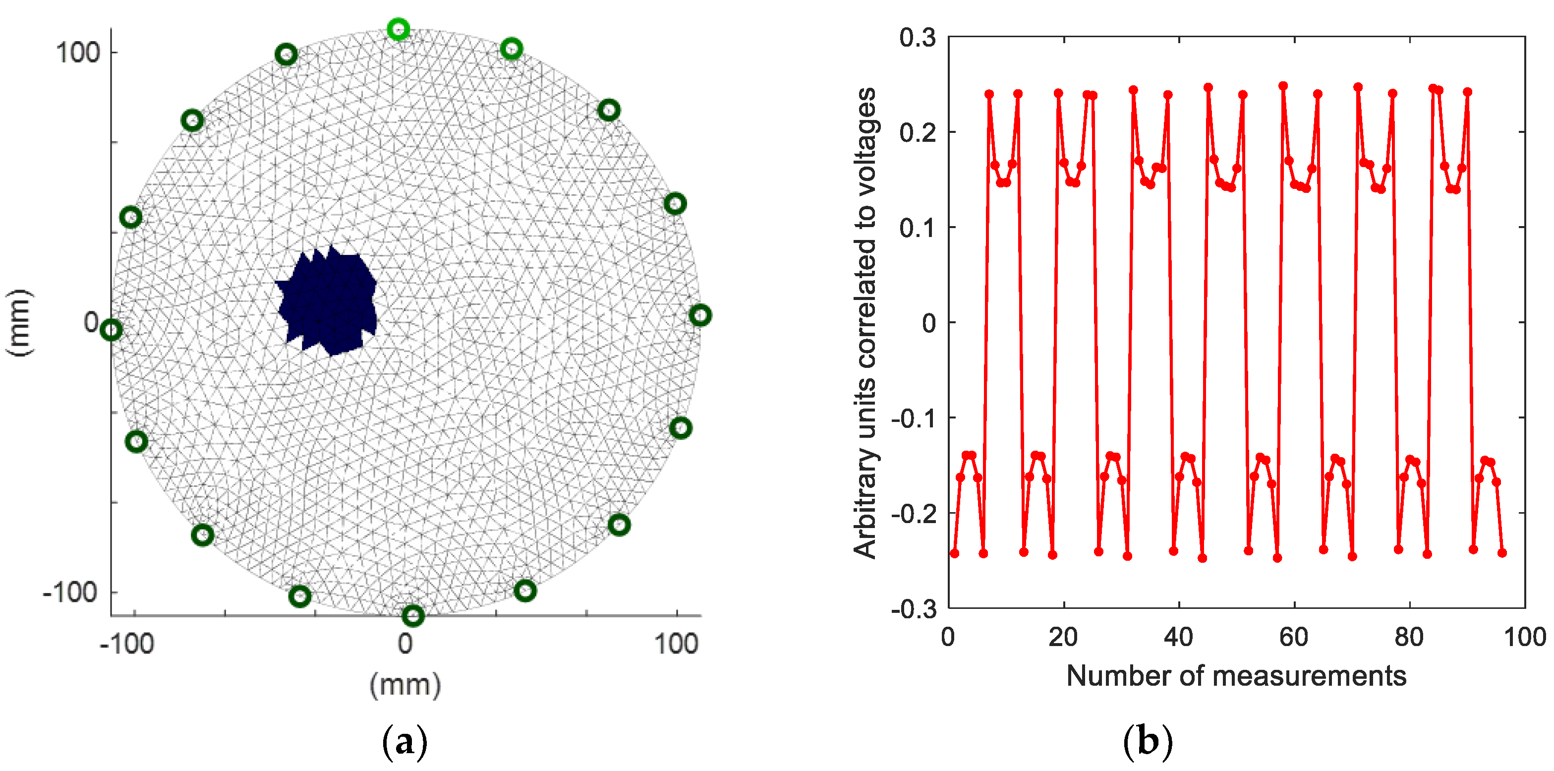
Figure 3 shows one of the 35,000 generated cases used to train the predictive system. The cross-section of the tank contains one random inclusion. Inclusion is visible through the variety of colours on the 2883 finite element mesh.
The colours correspond to conventional units corrected for the electrical conductivity of the interior of the tested object. Ninety-six voltage measurements were assigned to the conductivity values (Figure 3b). These are not the voltage values, but the arbitrary units correlated with them. As the polarity of the electrodes changes during individual measurements, the voltage changes in the range (−0.3; +0.3). Each measurement’s value was boosted by the addition of Gaussian noise with a standard deviation of 4%. Finite elements (pixels) in the image have the values 1 (for background) or 10 5 (for plastic tubes).

2.3. The Concept of the Method Oriented Ensemble (MOE)

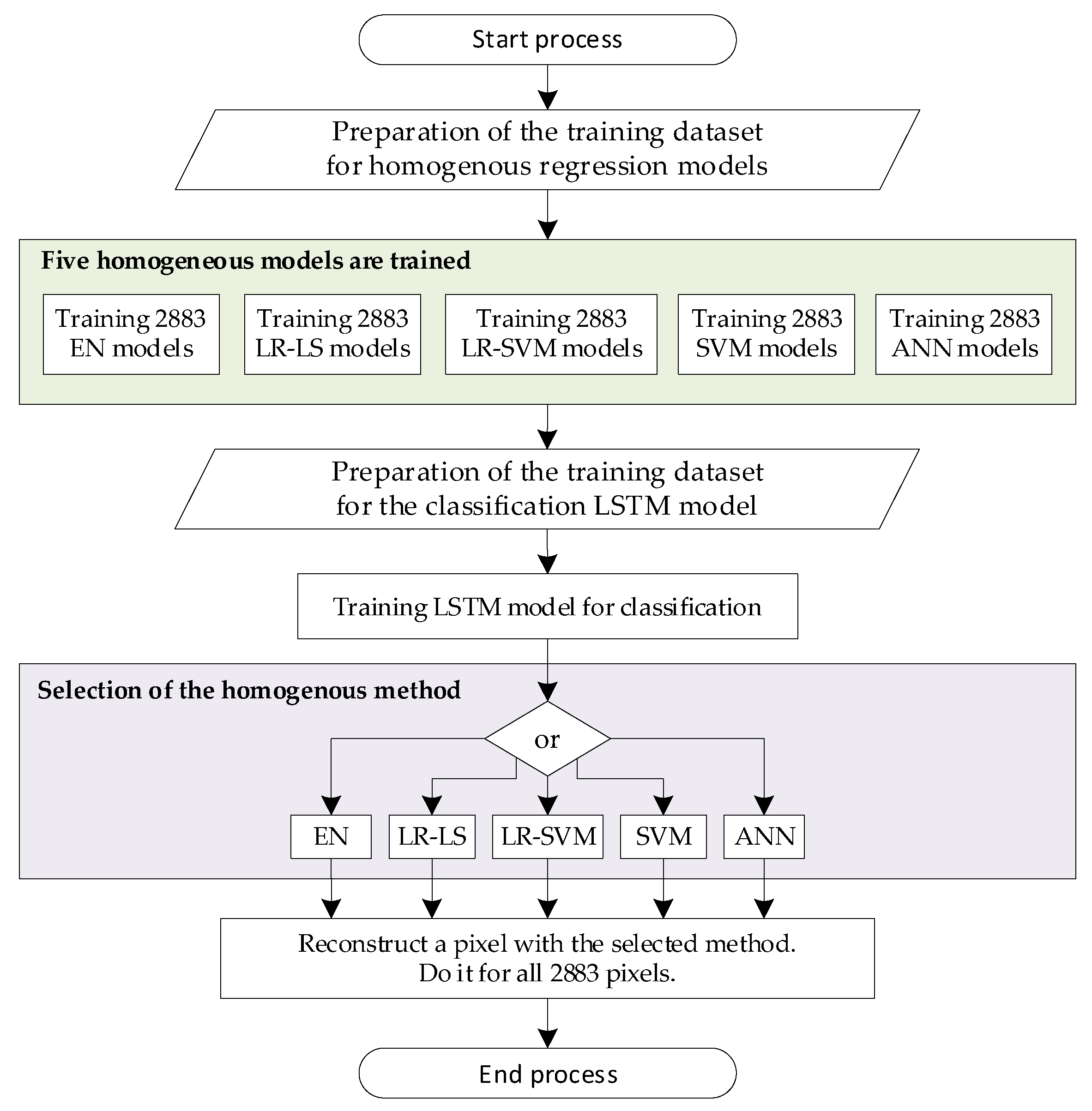
The proposed novel paradigm necessitates the training of several machine learning models for each pixel individually. Because the total number of pixels in the situation at hand is 2883, each of the five homogeneous approaches will require 2883 regression prediction models to be trained. Elastic Net (EN), Linear Regression with Least Squares learner (LR-LS), Linear Regression with Support Vector Machine learner (LR-SVM), Support Vector Machine (SVM), and Artificial Neural Network (ANN) are all used in the method-oriented ensemble (MOE) concept. The process of modelling the POE concept is presented in Figure 4. The presented flowchart is consistent with Algorithm 1 and Figure 1.
#Algorithm 1. The pseudocode algorithm for training MOE
1.
2.
3.
4.
5.
6.
7.
8.
9.
10.
11.
12.
13.
14.
15.
16.
17.
m = 96  % number of measurements
n = 2883 % number of finite elements in reconstruction mesh (pixels)
Train n models f 1 ( x 1 m ) y 1 n with method # 1 (e.g., EN)
Train n models f 2 ( x 1 m ) y 1 n with method # 2 (e.g., LR-LS)
Train n models f 3 ( x 1 m ) y 1 n with method # 3 (e.g., LR-SVM)
Train n models f 4 ( x 1 m ) y 1 n with method # 4 (e.g., SVM)
Train n models f 5 ( x 1 m ) y 1 n with method # 5 (e.g., ANN)
% Assigning the RMSE for each method and pixel
for i = 1:5  % for 5 methods: EN, LR-LS, LR-SVM, SVM, ANN
 for j = 1:n  % for n = 2883 pixels
  calculate RMSE(i, j)  % assignment root mean square error for i-th method and j-th pixel
 end
 meanRMSE(i) = mean(RMSE(i,:)) % Calculate the mean RMSE for each of the 5 methods.
end      % Assignment meanRMSE for i-th method and all 2883 pixels.
Prepare the training set to train the LSTM classifier. Inputs—96 measurements. Output—5 categories/classes.
Select the method with the lowest meanRMSE.
Reconstruct all n pixels using the selected method.
Algorithm 1 presents pseudocode to train a method-oriented ensemble (MOE) model. Based on 96 data, a specially trained LSTM classifier determines which of the five homogenous approaches (EN, LR-LS, LR-SVM, SVM, or ANN) is best for a given measurement situation (vector 96 measurements). It is worth noting that training five predictive models for each of the 2883 pixels yield 14,415 models. To this value, add the LSTM technique classifier. High computational complexity characterizes the new MOE idea. However, compared to the enormous improvement in image reconstruction quality that can be attained, this is a minor nuisance.

2.4. Elastic Net (EN)

When reconstructing tomographic images of real objects with low conductivity, the electrode data are frequently noisy. It is due to electrode insulation imperfections, the impacts of fast-varying, low-intensity currents created by multiplexers, the effects of electromagnetic fields, and various other reasons. Industrial reactors are another example of technological devices with a high noise level as determined by tomographic data. Electrical signal interference is one of the primary impediments to developing tomographic methods for such objects [41].
The elastic net regularization technique made the input data more robust to noise and distortions [42]. We begin with a linear system described by the equation of state Y = X β + ε , where Y R n is the matrix of output variables (reconstruction), X R n × ( k + 1 ) is the matrix of input variables, the coefficient β R k + 1 denotes a vector with unknown parameters, and ε R n reflects the sequence of the disturbance.
Elastic net is a compromise between L1 and L2 norms, or, to put it another way, between Robert Tibshirani’s LASSO (Least Absolute Shrinkage and Selection Operator) and ridge regression is known as Tikhonov regularization. The approach is also successful when there are numerous correlated predictors or when the number of discretized current elements is substantially more significant than the number of measurement points. Task (1) can be used to indicate the problem that determines the elastic net:
min ( β 0 , β ) R i + 1 1 2 n i = 1 n ( y i β 0 x i β ) 2 + λ P α ( β ) ,
where ( y i β 0 x i β ) are the linear model residuals, x i is the vector of measurements, y i is the vector of reference values, β 0 is the intercept equal to the mean of the response variable parameter, β denotes unknown parameters, λ is the parameter that specifies the penalty for regularization, and P α is a net elastic penalty defined by (2).
P α ( β ) = ( 1 α ) 1 2 β L 2 + α β L 1 ,
If the linear problem (1) has a solution in which the regression line intersects the y axis, then the unit column vector is the first column of the X matrix in the linear equation Y = X β + ε . The elastic net penalty P α is a summary combination of the L1 and L2 norms of unknown parameters β , as shown by Equation (2). The trade-off between LASSO and ridge regression is represented by parameter 0 α 1 . It is pure ridge regression if the value is α = 0 , but it is pure LASSO if the value is α = 1 .

2.5. Linear Regression with Least-Squares Learner (LR-LS)

A linear regression-based form of the approach was employed in the investigation. The SVM learner has been substituted by the least-squares model [43]. The algorithm employed in the LR-LS method is quite similar to the methodology employed in the previously disclosed LR-SVM method. In this instance, LASSO regression with L1 regularization was also utilized, as was the LASSO regression model without regularization. The distinction between LR-SVM and LR-LS is the loss function used to calculate the likelihood ratio. For LR-LS, the loss function is mean square error, which can be calculated as M S E = [ y , f ( x ) ] = 1 2 [ y f ( x ) ] 2 with the range of answers y ( , ) . In LR-LS, the deviation b equals the y-weighted median of all training processes multiplied by the number of training processes.

2.6. Linear Regression with Support Vector Machine Learner (LR-SVM)

The linear regression (LR) and support vector machines (SVM) algorithms are used in the LR-SVM algorithm [44]. The algorithm has been tuned to work best with the multidimensional vectors of data provided as input. This strategy, known as the L1 LASSO regularization technique, employs a regression model that incorporates the “absolute value of magnitude” into the loss function as a penalty component. In this study, the “learner” was a linear regression model based on the SVM approach, which was utilized [45]. f ( x ) = x β + b is the loss function for a linear regression model type, where β denotes a vector of pp coefficients, x denotes an observation of p predictor variables, and b denotes a scalar bias. The mean square error (MSE) is determined as a loss function in the implemented algorithm, and it takes the form of the formula [ y , f ( x ) ] = max [ 0 ,   | y f ( x ) | ε ] where y ( , ) is a reconstruction of the response value. The LASSO cost function is represented by the Equation (3)
min β 0 , β ( i = 1 n ( y i b x i T β ) 2 2 n + λ j = 1 p | β j | ) ,
where the number of observations is given by n. The transposed vector of length p at observation i is given by x i T . The reconstruction of a pixel at the observation vector gives y i . The regularization parameter is given by λ , which must be non-negative. In this study, the value of Lambda is λ = 1 / n . It is worth noting that the parameters b and β are in that order a scalar bias and a vector of length p, respectively. The number of non-zero β parameters reduces as the value grows. Regularized support vector machines (SVM) and least-squares regression methods are both included in the LR-SVM. The model minimizes the objective function by employing stochastic gradient descent (SGD), reducing the time required for computation. A ridge penalty is applied to support vector machines in the outlined method, which is then optimized using a dual SGD for SVM. The formula represents the criterion for terminating the iteration process B t B t 1 B t < ϰ , where ϰ is the relative tolerance on linear coefficients β t , and bias term b t , and B t = [ β t , b t ] .

2.7. Support Vector Machine (SVM)

Support Vector Machines (SVM) are based on the premise that a decision space may be partitioned by erecting borders that separate objects belonging to various classes. Regression and classification problems may both be solved using SVM, a standard machine learning method. Vladimir Vapnik and his colleagues first proposed this idea in 1992. As a result, there are four types of SVM: classification type 1 (C-SVM), classification type 2 ( ε -SVM), regression type 1 ( ε -SVM), regression type 2 ( ν -SVM). Support vector models fall into one of these four categories ( ν -SVM). We use SVM regression analysis to find the functional dependence between a dependent variable y and its independent variable x. y = f ( x ) + n o i s e is the formula used in regression analysis since it assumes the relationship is of the deterministic type f ( x ) , with some random noise added on top of it. The main goal is to determine the function f form that best provides the dependent variable’s value in new scenarios that the SVM model has not previously “seen”. The learning test trains the SVM model system by putting it through its paces with a set of cases. According to the proposed theory, each SVM subsystem is responsible for generating a single pixel value. The total number of trained SVM models in an EIT system is equal to the output image resolution, which is ( 96 SVM 1 ) × 2883 . As a result, the technique utilized in this study implements the regression type 2 problem (also known as the ν -SVM). The Equation (4) ’s deviation function is minimized [44]:
1 2 w T w C ( ν ε + 1 N i = 1 N ( ξ i + ξ i * ) ) ,
under the following conditions (5):
{ ( w T Φ ( x i ) + b ) y i   ε + ξ i   y i ( w T Φ ( x i ) + b i ) ε + ξ i * ξ i , ξ i * 0 ,       i = 1 , , N ,       ε 0 ,
where ε ,   ν are the penalty parameters, C is the capacity constant, w is a vector of coefficients, b is a constant, and ξ i ,   ξ i * are the overlapping case parameters. N learning examples are represented by index i independent variables are represented by x i , and regression patterns are represented by y i . The input data are converted to a new feature space via the kernel function. It is important to note that C significantly impacts the deviation, and its value must be carefully chosen to avoid overfitting the model. Each of the SVM subsystems was trained using 4000 training cases.

2.8. Artificial Neural Network (ANN)

The researchers employed artificial neural networks in the form of a multilayer perceptron for their investigation. The collection of 35,000 examples has been separated into three subsets: training, validation, and testing, with an aspect ratio of 70:15:15. The training subset contains cases that have been validated and assessed. As a result, 2883 models were trained, which is the same number of models as the resolution of the spatial tomographic image. Additionally, to optimize the models, a backward propagation of errors approach using conjugate gradients was utilized in conjunction with conjugate gradients. The structure of a single ANN dedicated to each of the 2883 pixels is 96-10-1. Ninety-six measurements are input to the network, ten neurons are in the hidden layer, and one regression neuron is in the output. The transfer function of the hidden layer is a hyperbolic tangent tanh ( x ) = e 2 x 1 e 2 x + 1 . The output layer makes use of a linear activation technique.

2.9. The Long Short-Term Memory (LSTM) Network for Classification

The classification of measurement cases to homogenous methods within MOE was accomplished using a deep LSTM network. This method differs from previous methods because it can learn long-term correlations between time steps in a time series or provided sequences. Furthermore, the measurement vector is used as a sequence of input variables to the recurrent deep LSTM neural network, a novel technique. The study’s findings demonstrated that such a strategy is quite effective in selecting the ideal homogenous method within MOE, as demonstrated by the study results.
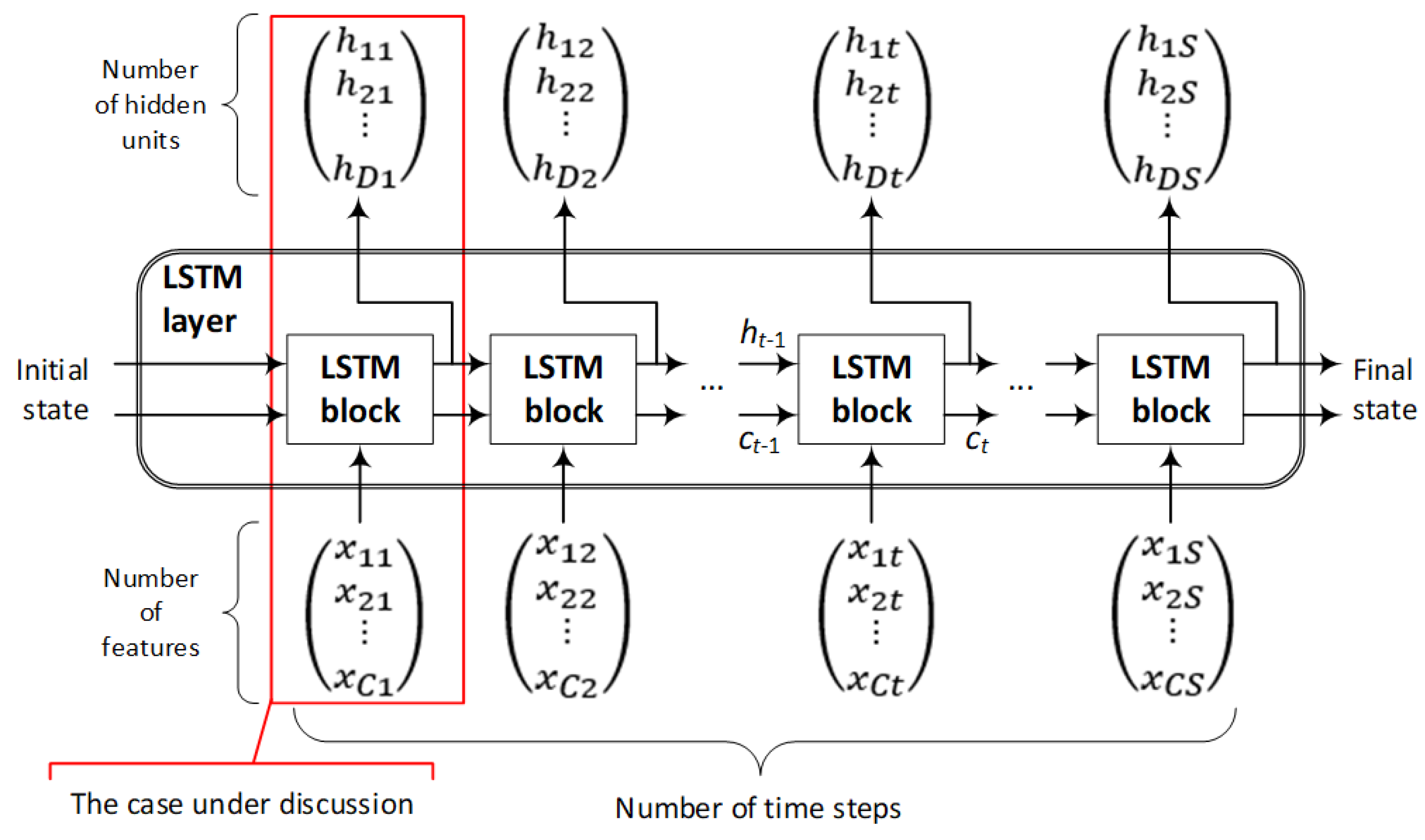
Illustration of a time series X flow with C features (channels) of length S through an LSTM layer, as depicted in Figure 5. The output (also known as the hidden state) and the cell state at time step t are represented by the symbols ht and ct, respectively, in the diagram [46]. For example, the first LSTM block considers both the network’s starting state and the first time step of the sequence to compute both the first output and the updated cell state. To compute the output and the updated cell state ct at time step t, the block uses the current state of the network (ct−1, ht−1) and the next time step in the series (time step t).
The hidden state (also known as the output state) and the cell state are the two states that make up the state of the layer. The output of the LSTM layer for the time step t is stored in the hidden state at time step t. In each time step, the cell state contains information that has been gained from the preceding steps in time. Thus, each time step, the layer either adds information to the cell state or removes information from the cell state, depending on the situation. The layer manages these changes through the use of gates. The cell state and concealed state of the layer are controlled by the following four components: input gate (i) that controls the level of cell state update, forget gate (f) that controls the level of cell state reset (forget), cell candidate (g) that adds information to cell state, and output gate (o) that controls the level of cell state added to hidden state.
The flow of data at the time step t is depicted in Figure 6. The diagram illustrates how the gates forget, update, and output the cell and hidden states and how they interact with one another. The LSTM network with seven layers was used.
The gates provide additional information on the cell’s state. Equation (6) can be used to characterize the weights W, the recurrent weights R, and the biases b.
W = [ W i W f W g W o ] ,     R = [ R i R f R g R o ] ,     b = [ b i b f b g b o ]   .
The symbols i, f, g, and o signify input gate, forget gate, cell candidate, and output gate, respectively. The state of a cell at a particular time step t is denoted as c t = f t c t 1 + i t g t , where ⊙ represents the Hadamard product, or in other words, vector element-wise multiplication. At time step t, the hidden state is defined as h t = o t σ c ( c t ) , where σ c is the state activation function. The Equation (7) defines the LSTM layer’s components at time step t,
{ i t = σ g ( W i x t + R i h t 1 + b i )   f t = σ g ( W f x t + R f h t 1 + b f ) g t = σ c ( W g x t + R g h t 1 + b g ) o t = σ g ( W o x t + R o h t 1 + b o )   ,
where σ g denotes the gate activation function. The sigmoidal activation function was employed in both biLSTM layers (see Table 1). The Equation σ ( x ) = ( 1 + e x ) 1 can be used to express this type of function.
In the case of neural networks, there are no rigid criteria for picking network parameters (e.g., number of layers, number of hidden units in LSTM layers, normalization requirements, initial weights, and biases functions) for specific types of issues. Accordingly, the network and training parameters are selected empirically. It was likewise the case in this circumstance. Table 1 presents the neural network parameters for the classification of homogeneous methods, having two double LSTM layers, 128 hidden units each. The performed experiments demonstrated that a lesser number of hidden units causes a worsening of network quality while increasing the number of units and adding subsequent layers extends the learning process without creating an increase in the quality of the LSTM network.
The first layer of the LSTM model is sequence input. The sequence input layer tries to enter chronological data into the network. The next is the bidirectional layer BiLSTM. The bidirectional LSTM layer learns long-term correlations between signal time steps or sequence data in both ways (forward with feedback). These interactions are significant when there is a need for the network to learn from full-time series at each time step. The second is the batch normalization layer. The batch normalization operation normalizes the input data across all observations for each channel independently. The batch normalization employed between convolution and nonlinear operations such as BiLSTM speeds up the training of the convolutional neural network and minimizes the sensitivity to network initialization. The next layer is again the BiLSTM bi-directional layer. The fifth layer of the LSTM is fully connected. This layer multiplies the numerical input values by the weight matrix and also adds a vector of biases. Another layer is the softmax. A softmax layer applies a softmax function to the input. For classification problems, a softmax layer and a classification layer commonly follow the final fully connected layer. The last is a classification layer. This layer computes the cross-entropy loss for classification and weighted classification tasks with mutually exclusive classes. The layer infers the number of classes from the output size of the previous layer.
One or more fully linked layers are introduced following the convolution and downsampling layers in deep networks. When the input to a fully connected layer is a sequence, as with LSTM, the fully connected layer performs each stage independently. If the output of the layer preceding the fully connected layer is an array A1 of dimension X by Y by Z, then the output of the fully connected layer is an array A2 of size X’ by Y by Z. The proper input to A2 at time step t is WA t + b , where A t is the time step t of A and b is the bias. Glorot initializer was used to generate the weights for this layer in this research [47]. The softmax is the penultimate layer. It is a common type of layer in deep categorization neural networks. An ultimately linked layer is always preceding the softmax layer. The formula y r ( x ) = e a r ( x ) / j = 1 k e a j ( x ) denotes the softmax activation function, with 0 y r 1 , and j = 1 k y j = 1 .
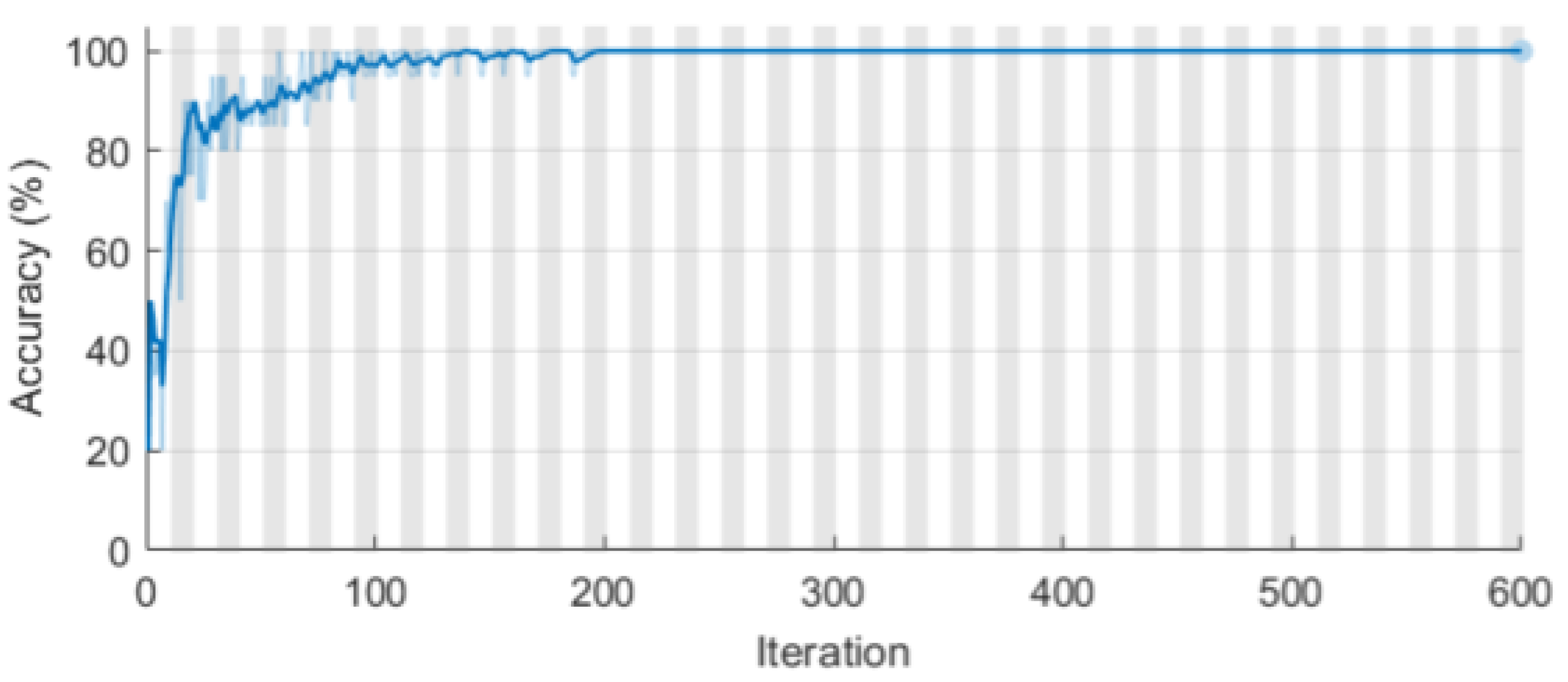
For classification problems with mutually exclusive classes, the final layer computes the cross-entropy loss. To ensure a sufficient number of training sets, aggregation of measurement data with comparable properties was performed. The LSTM network was trained using the adaptive moment estimation (ADAM) algorithm [48]. The following parameters apply to the BiLSTM layer: Tanh function for state activation, sigmoid function for gate activation, mini-batch size = 100, starting learning rate = 0.01, sequence length = 96 (longest), gradient threshold = 1. The parameters listed above were determined empirically. With a probability range from 0.1 to 0.5, various model variants featuring the dropout layer were examined. The experiments revealed that increasing dropout layers did not affect the network’s generalization in the scenario analyzed. As a result of the preceding, we opted against incorporating this layer into the proposed prediction model. The training status of the LSTM network using a raw input is depicted in Figure 7.
Cross-entropy and accuracy were used to assess the LSTM model’s quality. Accuracy is defined as the proportion of correctly identified observations across all instances (8).
A c c u r a c y = N c N · 100 %   ,
where Nc is the number of correctly rebuilt pixels, and N is the total number of pixels [49]. Equation (9) defines the cross-entropy loss between network predictions and target values
L o s s = i = 1 M T i l o g ( X i ) / N   ,
where N is the number of observations, M is the number of responses, Ti is the number of patterns, and Xi is the number of network outputs. The training-progress graphic demonstrates the correctness of the training. Indeed, it indicates the accuracy of each minibatch’s classification. This number increases to 100% for optimal training development. At the finish of the training procedure, the classifier’s accuracy oscillates between 99% and 100%. It took approximately 12 min to train. The computation was carried out on a personal computer configured as follows: 2.80 GHz Intel® CoreTM i5-8400 CPU, 16 GB RAM, NVIDIA GeForce RTX 2070 GPU. Parallel computing with GPU was used [50,51].
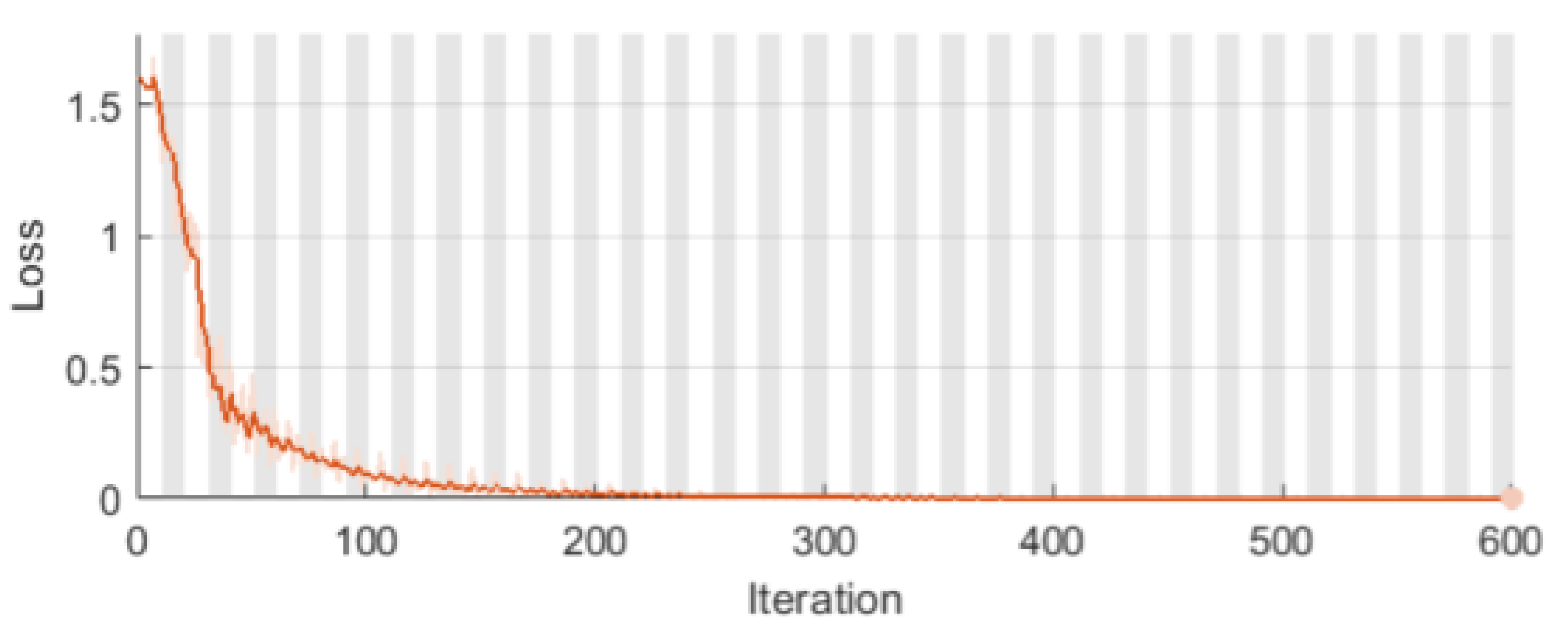
The LSTM learning process using a measurements vector as a signal in conjunction with the Loss indicator is illustrated in Figure 8. The graph depicts the training loss, which is the cross-entropy loss for each mini-batch. When training is carried out precisely, the loss should be zero. The shape of this plot corroborates all of the information in Figure 7.
Both Figure 7 and Figure 8 show a very high quality of the LSTM classifier. Curve shapes resembling a logarithm and a hyperbola, without fluctuations, are proof of the correct course of the learning process.
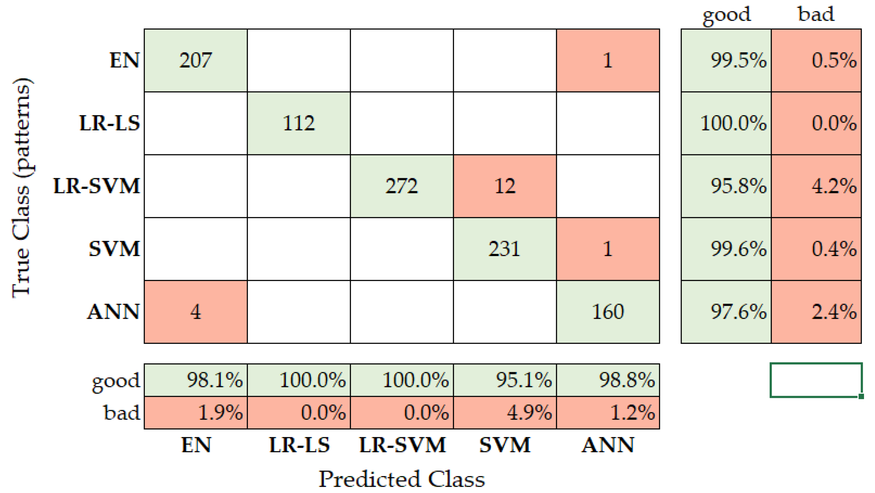
Figure 9 shows the confusion matrix of the LSTM classifier on the set of 1000 test cases. As can be seen, significant problems were caused by the correct classification of the EN method because 13.6% of the answers were incorrectly categorized as the ANN method. Thus, cumulative accuracy for the entire testing set was 98.2%.

3. Results and Discussion

Experiments were carried out to reconstruct EIT measurements based on real and simulation data to verify the effectiveness of the new MOE method. The first experiment was to visualize the inside of a physical model for three different scenarios. In the first case, two tubes were immersed in the water. In the second case, the position of the tubes was changed, and their number increased to three. Finally, the fourth case included four tubes arranged symmetrically at equal distances and the walls of the water container.
Reconstructions based on real measurements do not allow for objective comparisons due to the lack of reference images. Therefore, a series of experiments based on simulation data was also carried out to allow for an objective, index-based assessment that allows the comparison of individual reconstructions. In this way, the quality of the proposed MOE method was verified using error, deviation and correlation indicators.

3.1. Visualizations of Real Measurements

Figure 10 shows a schematic diagram of the physical model of the tested tank. Figure 10a shows a dimensioned side view of the cylinder with the tube submerged. Figure 10b–d show top views of the test tank with three cases of differently distributed inclusions. The considered measurement cases contain 2, 3 and 4 tubes, respectively, immersed in the cylinder. The diameter of the tested cross-section of the tank model is 32.5 cm. When submerged in water, the diameter of the plastic tube is 28 mm. 16 electrodes were evenly spaced around the cylinder at the height of 14 cm from the bottom.
Figure 11 shows the reconstructed three measurement cases presented earlier in Figure 10. The LSTM classifier indicated the SVM method in all tested cases. As is known, there is always a certain level of data noise in the case of real measurements. It makes this type of reconstruction more difficult to reconstruct than imaging simulation measurements. In Figure 11a, an artefact appears in the central part of the tank, but it is less pronounced than the images of the two tubes. The other reconstructions Figure 11b,c are successful.

3.2. Comparison of the Reconstructions Based on Simulation Data

Four widely used metrics were used to evaluate the quality of tomographic reconstructions objectively: Root Mean Square Error (RMSE), Relative Image Error (RIE), Percentage Error (PE), Mean Absolute Percentage Error (MAPE), and Image Correlation Coefficient (ICC). The root mean square error is calculated using the Equation (10)
RMSE = i = 1 n ( y i y ^ i ) 2 n   ,
where n is the number of finite elements or the picture resolution, y i denotes the i-th pixel’s pattern conductivity, and y ^ i denotes the reconstruction conductivity. RIE is calculated as (11)
RIE = y y y   ,
where y is the ground-truth (reference) conductivity distribution and y is the reconstructed conductivity distribution. MAPE is calculated using the following Eqaution (12)
MAPE = 1 n i = 1 n | y y ^ y | .
The ICC metric describes the function (13)
ICC = i = 1 n ( y i y ¯ ) ( y ^ i y ^ ¯ ) i = 1 n ( y i y ¯ ) 2 i = 1 n ( y ^ i y ^ ¯ ) 2   ,
where y ¯ denotes the mean reference ground-truth conductivity distribution and y ^ ¯ denotes the mean EIT reconstruction conductivity distribution.
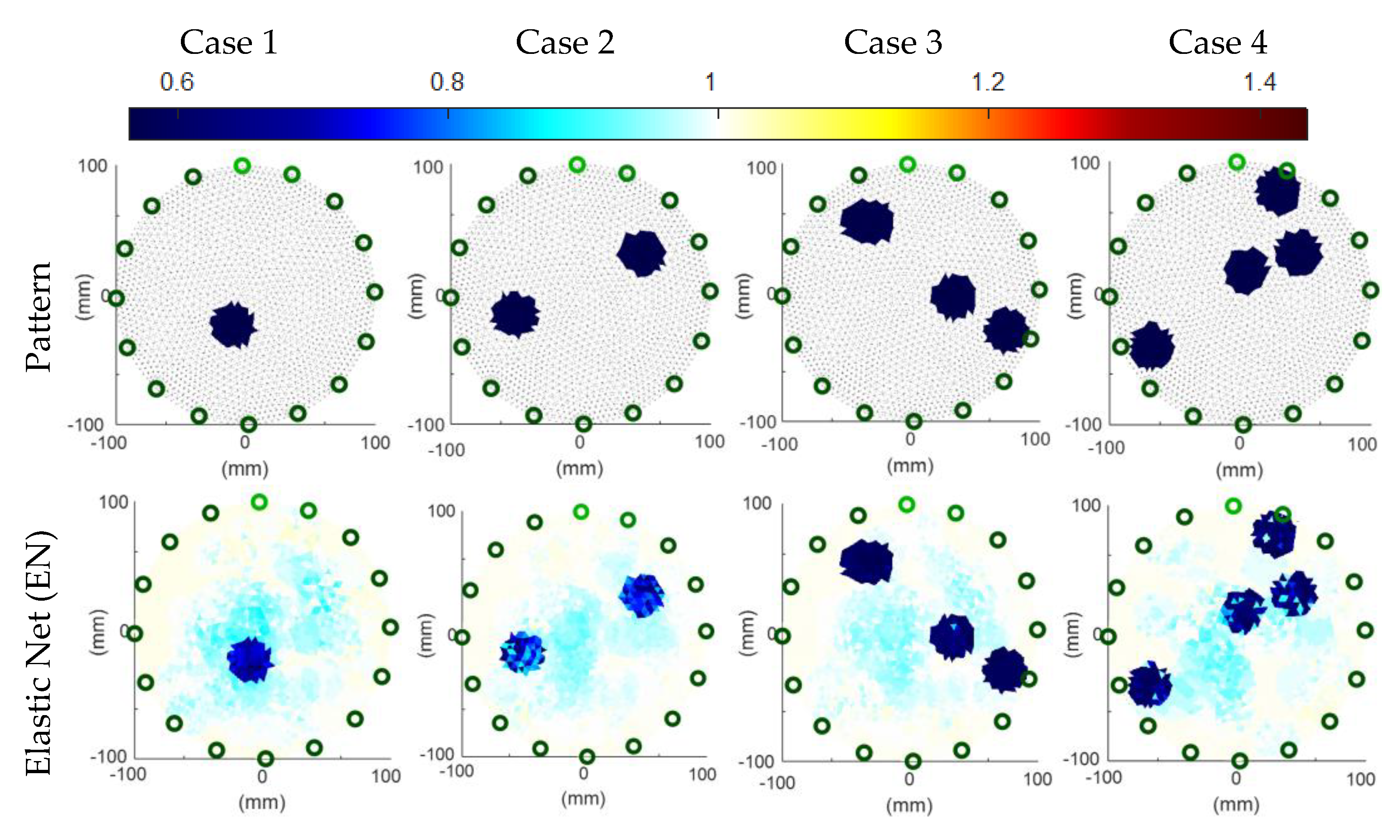
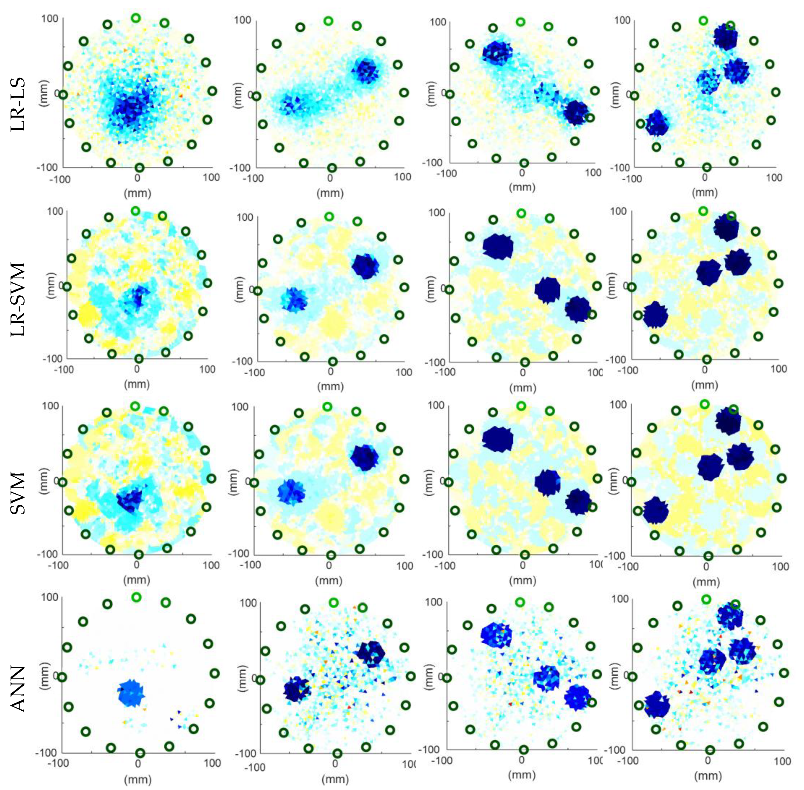
The lower the root mean square error, the smaller the RIE, and the greater the MAPE value, the higher the tomographic image quality. Thus, ICC = 1 indicates perfect reconstruction, whereas ICC = 0 indicates the worst-case scenario. Reconstructions based on simulation measurements are shown in Figure 11. The first line of Figure 11 illustrates the reference images of the model tested. Reconstructions using homogeneous EN, LS-SVM, LR-LS, SVM and ANN methods are shown in the following lines.
Table 2 corresponds with Figure 12. Table 2 presents quantitative indicators that enable the comparison of individual homogeneous methods included in the new MOE concept. The best values of indicators are marked in blue.
Visual (subjective) observation of the images in Figure 12 concludes that the best reconstructions were obtained by the EN and ANN methods for the first measurement case with a single inclusion. According to the indicators included in Table 2, the best method is ANN. The second case of measurement is not so clear-cut. In Table 2, according to the RMSE and RIE indicators, the best is the SVM reconstruction, according to MAPE-ANN and ICC-EN. Notably, any indicators did not select the LR-LS and LR-SVM methods, which visually look worse than the others. The third case, with three inclusions, according to RMSE and RIE, is best reconstructed by the LR-SVM method, according to MAPE-SVM, and according to ICC-EN. Visual observation confirms the rightness of this choice. In the last, fourth measurement case, all indicators in Table 2 indicated the superiority of the LR-SVM method. It can be seen that the SVM method fares very similarly, although it is worse. Visual observation of Figure 12 can confirm this. Since the purpose of tomography is not a precise measurement of electrical conductivity inside the tested objects but an accurate, precise, and quick visualization of inclusions, the MAPE index, as an index reflecting the absolute values of the patterns and reconstructions, should be treated as optional/supplementary. Large values of the MAPE index result from 2883 pixels included in the tomographic image and the fact that the reference background values are “1” and the inclusions are close to zero (precisely 10−5).
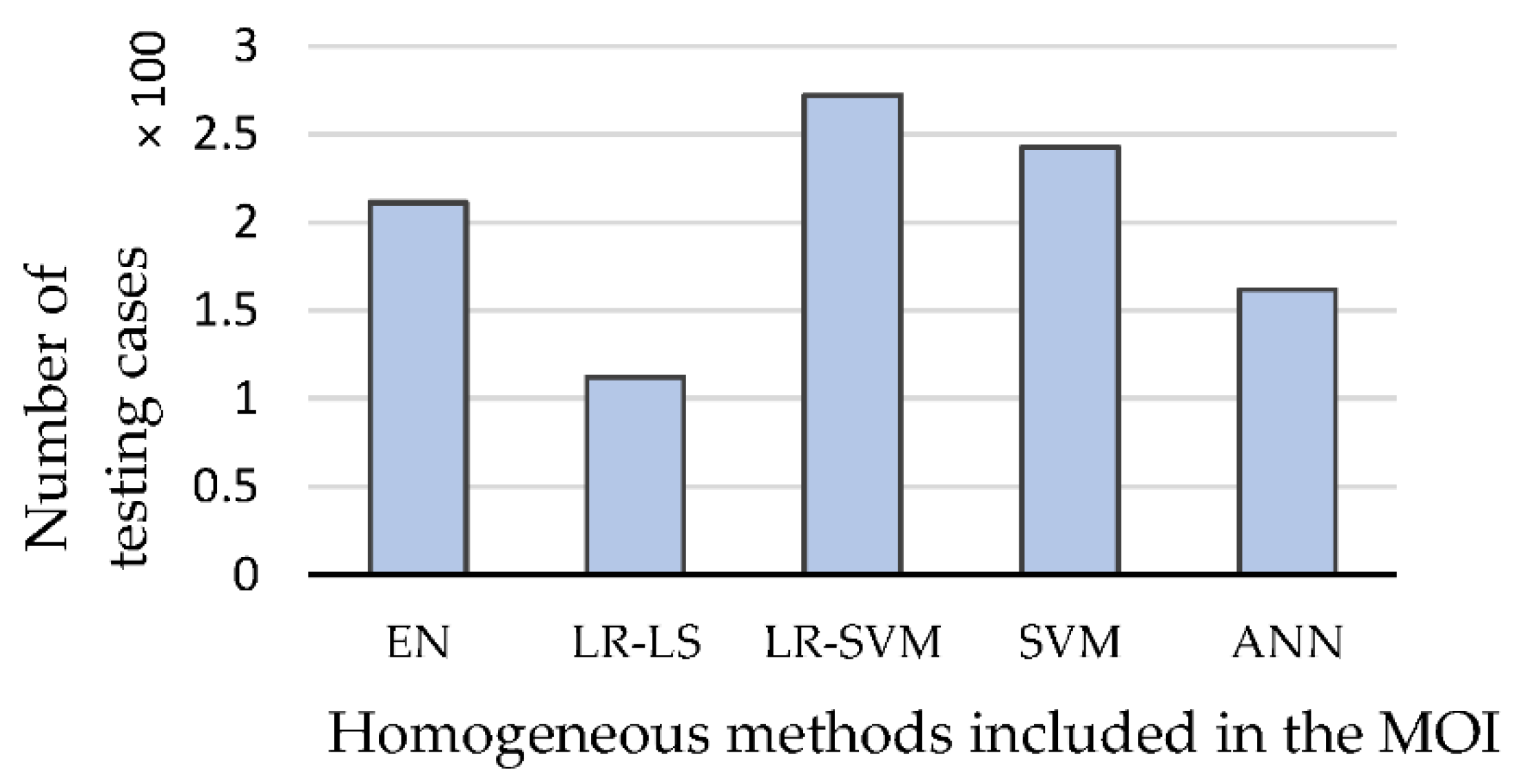
Figure 13 shows the 1000-item testing set broken down by quantity for each homogeneous method selected by the LSTM classifier. As can be seen, in the test set under consideration, the LR-SVM method was indicated the most times, while the LR-LS method was chosen the least frequently. It should be noted that the method quality indicator for the LSTM classifier was the RMSE. Impedance tomography is a potential field of science for identifying inclusions inside industrial reactors, containers, and pipes [52,53]. The presented research findings substantiate the preceding assertion due to the complexity of the model transferring the measurement data into the output image and the requirement to solve the incorrectly stated inverse problem, developing an effective and universal technique. The novel MOE approach described in this article uses considerable computational resources to maximize the resulting image’s quality. With the ongoing development of new mathematical homogenous methods, hybrid (ensemble) methods should not be overlooked. In this regard, the MOE technique is more advanced. MOE makes every effort from the start to fully use the data available in the measurement data collection. Because distinct training models are used for each pixel in the output image, each pixel’s value, and hence the colour, is calculated using the entire vector of 96 measurements.
Perfect results were obtained due to the unconventional deployment of a recurrent LSTM network. The most often utilized use of LSTM is to process time series and sequences. Therefore, we considered the measurement vector a collection of structured data (sequence) with a single step in our research. This technique proved correct, as indicated by the near-perfect classification of homogeneous methods using the MOE method.
Differences in image reconstruction across separate models are due to different methods, but not exclusively. For instance, when a homogeneous approach (e.g., elastic net or SVM) is used with the same input vector for all pixels, reconstructing an image with 2883 pixels requires adjusting the parameter values and hyperparameters of models trained for specific finite elements (pixels).
The objective of machine learning methods is to extract pure information from input data. It is information that can be used to create the output image successfully. There are numerous methods for obtaining the information’s essence. Preprocessing can be used to clean, standardize, encode and decode, increase or shrink, and extract features from data. It turns out that to get the highest possible reconstruction quality, the number of iterations and variation of the model can also be multiplied. This approach is superior to typical pre-processing procedures in that it is applicable to practically any problem. As a result, the tomographic images of the inclusion distribution inside the reactors are more precise, legible, and have a more excellent resolution. It is one of the benefits of the novel MOE concept described in this paper.

4. Conclusions

This publication provides a new algorithmic MOE method that optimizes EIT reconstructions in industrial applications simultaneously using many machine learning methods. Moreover, the provided method permits the visualization of the distribution of inclusions inside the tested reactor.
The fundamental aspect that distinguishes MOE from other methods is the high chance of increasing the quality of reconstructive images without using new, previously unknown homogenous methods. MOE is the concept of making greater use of computing resources and offering alternative methods. To apply the novel MOE methodology, it is enough to train a few models that use existing prediction methods, such as SVM, linear regression, neural networks, decision trees, elastic net, LASSO, k-nearest neighbours, etc. and then use them as stated in this article. Regardless of how many methods are employed in the MOE, it is almost assured that the results achieved will be better than if each homogenous approach was utilized alone. An exciting discovery is the unusual use of the LSTM network as a method classifier. This was made possible by treating the measurement vector as a succession of measurements.
Future studies will be carried out to improve the MOE approach with increased usage of deep learning and recursive neural networks.

Author Contributions

Development of the system concept, measurement methodology, image reconstruction and supervision, T.R.; Development of software for mathematical models and the measurement concept of electrical impedance tomography for industrial tomography research, G.K.; Development of a measurement concept in a real model of a tank reactor, preparation of a measuring station, measurements, development of measurement methodology, preparation of descriptions in the article, M.M. and A.D.; Development of the numerical methods and techniques, K.N.; Literature review, formal analysis, general review, and editing of the manuscript, M.R. All authors have read and agreed to the published version of the manuscript.

Funding

This research received no external funding.

Institutional Review Board Statement

Not applicable.

Informed Consent Statement

Not applicable.

Data Availability Statement

Kłosowski, Grzegorz (2021), “Training dataset”, Mendeley Data, V1, doi: 10.17632/4hjt9dzcvd.1.

Conflicts of Interest

The authors declare no conflict of interest.

References

  1. Park, S.; Na, J.; Kim, M.; Lee, J.M. Multi-objective Bayesian optimization of chemical reactor design using computational fluid dynamics. Comput. Chem. Eng. 2018, 119, 25–37. [Google Scholar] [CrossRef]
  2. Kosicka, E.; Kozłowski, E.; Mazurkiewicz, D. Intelligent Systems of Forecasting the Failure of Machinery Park and Supporting Fulfilment of Orders of Spare Parts. In Proceedings of the First International Conference on Intelligent Systems in Production Engineering and Maintenance ISPEM, Wrocław, Poland, 28–29 September 2017; pp. 54–63. [Google Scholar]
  3. Wang, M. Industrial Tomography: Systems and Applications; Elsevier: Amsterdam, The Netherlands, 2015; ISBN 1782421181. [Google Scholar]
  4. Wajman, R.; Banasiak, R.; Babout, L. On the Use of a Rotatable ECT Sensor to Investigate Dense Phase Flow: A Feasibility Study. Sensors 2020, 20, 4854. [Google Scholar] [CrossRef] [PubMed]
  5. Ye, Z.; Banasiak, R.; Soleimani, M. Planar array 3D electrical capacitance tomography. Insight Non-Destr. Test. Cond. Monit. 2013, 55, 675–680. [Google Scholar] [CrossRef]
  6. Mosorov, V.; Rybak, G.; Sankowski, D. Plug Regime Flow Velocity Measurement Problem Based on Correlability Notion and Twin Plane Electrical Capacitance Tomography: Use Case. Sensors 2021, 21, 2189. [Google Scholar] [CrossRef] [PubMed]
  7. Romanowski, A.; Chaniecki, Z.; Koralczyk, A.; Woźniak, M.; Nowak, A.; Kucharski, P.; Jaworski, T.; Malaya, M.; Rózga, P.; Grudzień, K. Interactive Timeline Approach for Contextual Spatio-Temporal ECT Data Investigation. Sensors 2020, 20, 4793. [Google Scholar] [CrossRef] [PubMed]
  8. Voss, A.; Pour-Ghaz, M.; Vauhkonen, M.; Seppänen, A. Retrieval of the saturated hydraulic conductivity of cement-based materials using electrical capacitance tomography. Cem. Concr. Compos. 2020, 112, 103639. [Google Scholar] [CrossRef]
  9. Garbaa, H.; Jackowska-Strumiłło, L.; Grudzień, K.; Romanowski, A. Application of electrical capacitance tomography and artificial neural networks to rapid estimation of cylindrical shape parameters of industrial flow structure. Arch. Electr. Eng. 2016, 65, 657–669. [Google Scholar] [CrossRef]
  10. Grudzien, K.; Chaniecki, Z.; Romanowski, A.; Sankowski, D.; Nowakowski, J.; Niedostatkiewicz, M. Application of twin-plane ECT sensor for identification of the internal imperfections inside concrete beams. In Proceedings of the 2016 IEEE International Instrumentation and Measurement Technology Conference, Taipei, Taiwan, 23–26 May 2016; pp. 1–6. [Google Scholar] [CrossRef]
  11. Kryszyn, J.; Smolik, W.T.; Radzik, B.; Olszewski, T.; Szabatin, R. Switchless charge-discharge circuit for electrical capacitance tomography. Meas. Sci. Technol. 2014, 25, 115009. [Google Scholar] [CrossRef]
  12. Kryszyn, J.; Smolik, W. Toolbox for 3D modelling and image reconstruction in electrical capacitance tomography. Inform. Control. Meas. Econ. Environ. Prot. 2017, 7, 137–145. [Google Scholar] [CrossRef]
  13. Majchrowicz, M.; Kapusta, P.; Jackowska-Strumiłło, L.; Sankowski, D. Acceleration of image reconstruction process in the electrical capacitance tomography 3D in heterogeneous, multi-GPU system. Inform. Control. Meas. Econ. Environ. Prot. 2017, 7, 37–41. [Google Scholar] [CrossRef]
  14. Romanowski, A. Big Data-Driven Contextual Processing Methods for Electrical Capacitance Tomography. IEEE Trans. Ind. Inform. 2019, 15, 1609–1618. [Google Scholar] [CrossRef]
  15. Soleimani, M.; Mitchell, C.N.; Banasiak, R.; Wajman, R.; Adler, A. Four-dimensional electrical capacitance tomography imaging using experimental data. Prog. Electromagn. Res. 2009, 90, 171–186. [Google Scholar] [CrossRef] [Green Version]
  16. Banasiak, R.; Wajman, R.; Jaworski, T.; Fiderek, P.; Fidos, H.; Nowakowski, J.; Sankowski, D. Study on two-phase flow regime visualization and identification using 3D electrical capacitance tomography and fuzzy-logic classification. Int. J. Multiph. Flow 2014, 58, 1–14. [Google Scholar] [CrossRef]
  17. Dusek, J.; Hladky, D.; Mikulka, J. Electrical impedance tomography methods and algorithms processed with a GPU. In Proceedings of the 2017 Progress in Electromagnetics Research Symposium—Spring (PIERS), St. Petersburg, Russia, 22–25 May 2017; pp. 1710–1714. [Google Scholar]
  18. Kłosowski, G.; Rymarczyk, T. Using neural networks and deep learning algorithms in electrical impedance tomography. Inform. Autom. Pomiary Gospod. Ochr. Sr. 2017, 7, 99–102. [Google Scholar] [CrossRef]
  19. Voutilainen, A.; Lehikoinen, A.; Vauhkonen, M.; Kaipio, J.P. Three-dimensional nonstationary electrical impedance tomography with a single electrode layer. Meas. Sci. Technol. 2010, 21, 35107. [Google Scholar] [CrossRef]
  20. Duraj, A.; Korzeniewska, E.; Krawczyk, A. Classification algorithms to identify changes in resistance. Przegląd Elektrotechn. 2015, 1, 82–84. [Google Scholar] [CrossRef]
  21. Szczesny, A.; Korzeniewska, E. Selection of the method for the earthing resistance measurement. Przegląd Elektrotechn. 2018, 94, 178–181. [Google Scholar]
  22. Dusek, J.; Mikulka, J. Measurement-Based Domain Parameter Optimization in Electrical Impedance Tomography Imaging. Sensors 2021, 21, 2507. [Google Scholar] [CrossRef]
  23. Chen, B.; Abascal, J.; Soleimani, M. Extended Joint Sparsity Reconstruction for Spatial and Temporal ERT Imaging. Sensors 2018, 18, 4014. [Google Scholar] [CrossRef] [Green Version]
  24. Liu, S.; Huang, Y.; Wu, H.; Tan, C.; Jia, J. Efficient Multitask Structure-Aware Sparse Bayesian Learning for Frequency-Difference Electrical Impedance Tomography. IEEE Trans. Ind. Inform. 2021, 17, 463–472. [Google Scholar] [CrossRef] [Green Version]
  25. Ziolkowski, M.; Gratkowski, S.; Zywica, A.R. Analytical and numerical models of the magnetoacoustic tomography with magnetic induction. COMPEL Int. J. Comput. Math. Electr. Electron. Eng. 2018, 37, 538–548. [Google Scholar] [CrossRef]
  26. Rymarczyk, T.; Adamkiewicz, P.; Polakowski, K.; Sikora, J. Effective ultrasound and radio tomography imaging algorithm for two-dimensional problems. Przegląd Elektrotechn. 2018, 94, 62–69. [Google Scholar]
  27. Liang, G.; Dong, F.; Kolehmainen, V.; Vauhkonen, M.; Ren, S. Nonstationary Image Reconstruction in Ultrasonic Transmission Tomography Using Kalman Filter and Dimension Reduction. IEEE Trans. Instrum. Meas. 2021, 70, 1–12. [Google Scholar] [CrossRef]
  28. Babout, L.; Grudzień, K.; Wiącek, J.; Niedostatkiewicz, M.; Karpiński, B.; Szkodo, M. Selection of material for X-ray tomography analysis and DEM simulations: Comparison between granular materials of biological and non-biological origins. Granul. Matter 2018, 20, 38. [Google Scholar] [CrossRef] [Green Version]
  29. Korzeniewska, E.; Sekulska-Nalewajko, J.; Gocławski, J.; Dróżdż, T.; Kiełbasa, P. Analysis of changes in fruit tissue after the pulsed electric field treatment using optical coherence tomography. Eur. Phys. J. Appl. Phys. 2020, 91, 30902. [Google Scholar] [CrossRef]
  30. Sekulska-Nalewajko, J.; Gocławski, J.; Korzeniewska, E. A method for the assessment of textile pilling tendency using optical coherence tomography. Sensors 2020, 20, 3687. [Google Scholar] [CrossRef] [PubMed]
  31. Sobaszek, Ł.; Gola, A.; Świć, A. Predictive Scheduling as a Part of Intelligent Job Scheduling System; Springer: Cham, Switzerland, 2018; pp. 358–367. [Google Scholar]
  32. Kłosowski, G.; Gola, A.; Świć, A. Application of fuzzy logic controller for machine load balancing in discrete manufacturing system. In Proceedings of the International Conference on Intelligent Data Engineering and Automated Learning, Wroclaw, Poland, 14–16 October 2015; Volume 9375, pp. 256–263. [Google Scholar]
  33. Rymarczyk, T.; Kłosowski, G.; Kozłowski, E. A Non-Destructive System Based on Electrical Tomography and Machine Learning to Analyze the Moisture of Buildings. Sensors 2018, 18, 2285. [Google Scholar] [CrossRef] [PubMed] [Green Version]
  34. Rymarczyk, T.; Kłosowski, G.; Hoła, A.; Sikora, J.; Wołowiec, T.; Tchórzewski, P.; Skowron, S. Comparison of Machine Learning Methods in Electrical Tomography for Detecting Moisture in Building Walls. Energies 2021, 14, 2777. [Google Scholar] [CrossRef]
  35. Lopato, P.; Chady, T.; Sikora, R.; Gratkowski, S.; Ziolkowski, M. Full wave numerical modelling of terahertz systems for nondestructive evaluation of dielectric structures. COMPEL Int. J. Comput. Math. Electr. Electron. Eng. 2013, 32, 736–749. [Google Scholar] [CrossRef]
  36. Psuj, G. Multi-Sensor Data Integration Using Deep Learning for Characterization of Defects in Steel Elements. Sensors 2018, 18, 292. [Google Scholar] [CrossRef] [PubMed] [Green Version]
  37. Kozłowski, E.; Mazurkiewicz, D.; Kowalska, B.; Kowalski, D. Binary linear programming as a decision-making aid for water intake operators. In Proceedings of the First International Conference on Intelligent Systems in Production Engineering and Maintenance ISPEM, Wrocław, Poland, 28–29 September 2017; Advances in Intelligent Systems and Computing Series. Springer: Cham, Switzerland, 2018; Volume 637, pp. 199–208. [Google Scholar]
  38. Yuen, B.; Dong, X.; Lu, T. Inter-Patient CNN-LSTM for QRS Complex Detection in Noisy ECG Signals. IEEE Access 2019, 7, 169359–169370. [Google Scholar] [CrossRef]
  39. Saadatnejad, S.; Oveisi, M.; Hashemi, M. LSTM-Based ECG Classification for Continuous Monitoring on Personal Wearable Devices. IEEE J. Biomed. Heal. Inform. 2019, 24, 515–523. [Google Scholar] [CrossRef] [PubMed] [Green Version]
  40. Adler, A.; Lionheart, W.R.B. Uses and abuses of EIDORS: An extensible software base for EIT. Physiol. Meas. 2006, 27, S25–S42. [Google Scholar] [CrossRef] [PubMed] [Green Version]
  41. Rymarczyk, T.; Kłosowski, G.; Kozłowski, E.; Tchórzewski, P. Comparison of Selected Machine Learning Algorithms for Industrial Electrical Tomography. Sensors 2019, 19, 1521. [Google Scholar] [CrossRef] [PubMed] [Green Version]
  42. Kryszyn, J.; Wanta, D.M.; Smolik, W.T. Gain Adjustment for Signal-to-Noise Ratio Improvement in Electrical Capacitance Tomography System EVT4. IEEE Sens. J. 2017, 17, 8107–8116. [Google Scholar] [CrossRef]
  43. Xiao, L. Dual averaging methods for regularized stochastic learning and online optimization. J. Mach. Learn. Res. 2010, 11, 2543–2596. [Google Scholar]
  44. Ho, C.H.; Lin, C.J. Large-scale linear support vector regression. J. Mach. Learn. Res. 2012, 13, 3323–3348. [Google Scholar]
  45. Hsieh, C.J.; Chang, K.W.; Lin, C.J.; Keerthi, S.S.; Sundararajan, S. A dual coordinate descent method for large-scale linear SVM. In Proceedings of the 25th International Conference on Machine Learning, Helsinki, Finland, 5–9 July 2008. [Google Scholar]
  46. Beale, M.H.; Hagan, M.T.; Demuth, H.B. Deep Learning Toolbox User’s Guide; The Mathworks Inc.: Herborn, Germany, 2018. [Google Scholar]
  47. Glorot, X.; Yoshua, B. Understanding the difficulty of training deep feedfor-ward neural networks. In Proceedings of the Thirteenth International Conference on Artificial Intelligence and Statistics, Sardinia, Italy, 13–15 May 2010; pp. 249–256. [Google Scholar]
  48. Kingma, D.P.; Ba, J.L. Adam: A method for stochastic optimization. In Proceedings of the 3rd International Conference on Learning Representations, ICLR 2015—Conference Track, San Diego, CA, USA, 7–9 May 2015. [Google Scholar]
  49. Kłosowski, G.; Rymarczyk, T.; Kania, K.; Świć, A.; Cieplak, T. Maintenance of industrial reactors supported by deep learning driven ultrasound tomography. Eksploat. Niezawodn. 2020, 22, 138–147. [Google Scholar] [CrossRef]
  50. Mikulka, J. GPU-Accelerated Reconstruction of T2 Maps in Magnetic Resonance Imaging. Meas. Sci. Rev. 2015, 15, 210–218. [Google Scholar] [CrossRef] [Green Version]
  51. Majchrowicz, M.; Kapusta, P.; Jackowska-Strumiłło, L.; Banasiak, R.; Sankowski, D. Multi-GPU, Multi-Node Algorithms for Acceleration of Image Reconstruction in 3D Electrical Capacitance Tomography in Heterogeneous Distributed System. Sensors 2020, 20, 391. [Google Scholar] [CrossRef] [PubMed] [Green Version]
  52. Rzasa, M.R.; Czapla-Nielacna, B. Analysis of the Influence of the Vortex Shedder Shape on the Metrological Properties of the Vortex Flow Meter. Sensors 2021, 21, 4697. [Google Scholar] [CrossRef] [PubMed]
  53. Shi, X.; Tan, C.; Dong, F.; Santos, E.N.D.; Silva, M.J. Da Conductance Sensors for Multiphase Flow Measurement: A Review. IEEE Sens. J. 2021, 21, 12913–12925. [Google Scholar] [CrossRef]
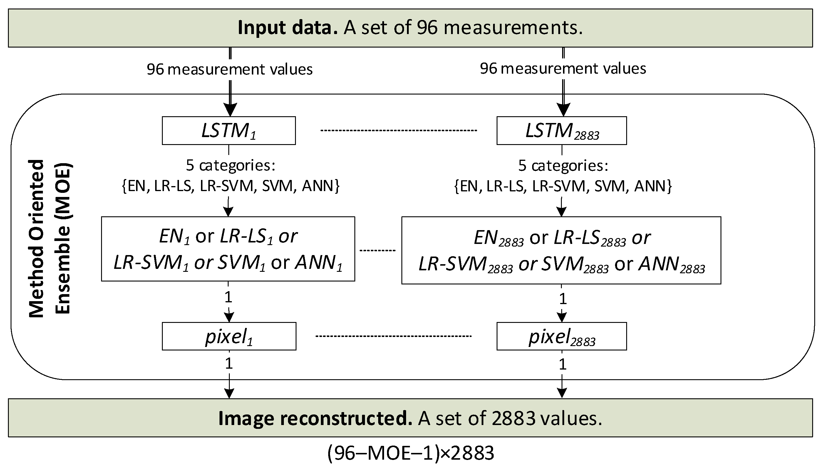
Figure 1. Principle of the Method Oriented Ensemble (MOE) concept.
Energies 14 07269 g001
Figure 2. The key elements of the test stand: (a)—electrical impedance tomograph connected to the electrodes; (b)—a physical model of a tank with plastic tubes immersed in water, (c)—cylinder diameter in (cm).
Energies 14 07269 g002
Figure 3. A sample training measurement case generated with the Eidors toolbox: (a)—cross-section with a visible inclusion; (b)—values of 96 measurements corresponding to the cross-section containing the inclusion.
Energies 14 07269 g003
Figure 4. The flowchart of new concept (MOE) modelling.
Energies 14 07269 g004
Figure 5. LSTM network structure for classification of raw electrical measurements.
Energies 14 07269 g005
Figure 6. Gates interaction in the LSTM network [46].
Energies 14 07269 g006
Figure 7. Training accuracy for LSTM network.
Energies 14 07269 g007
Figure 8. Training loss for LSTM network.
Energies 14 07269 g008
Figure 9. Confusion matrix for the testing set of the LSTM classification.
Energies 14 07269 g009
Figure 10. Real measurements: (a)—dimensioned test stand for real cases. Three variants of the arrangement of phantoms in the tested tank with 16 electrodes: (b)—2 phantoms, (c)—3 phantoms, (d)—4 phantoms.
Energies 14 07269 g010
Figure 11. Image reconstructions based on real measurements: (a)—a case with two inclusions, (b)—a case with three inclusions, (c)—a case with four inclusions.
Energies 14 07269 g011
Figure 12. Image reconstructions based on simulation measurements.
Energies 14 07269 g012aEnergies 14 07269 g012b
Figure 13. Results of the selections made by the LSTM classifier on a set of 1000 testing cases.
Energies 14 07269 g013
Table 1. Layers of LSTM network for classification with activations, learnable and states.
#Layer DescriptionActivationsLearnable Parameters
(Weights and Biases)
Total LearnablesStates
1Sequence input with 96 dimensions96-0-
2BiLSTM with 128 hidden units256Input weights: 1024 × 96
Recurrent weights: 1024 × 128
Bias: 1024 × 1
230,400Hidden state 256 × 1
Cell state 256 × 1
3Batch normalization256Offset: 256 × 1
Scale: 256 × 1
512-
4BiLSTM with 128 hidden units256Input weights: 1024 × 256
Recurrent weights: 1024 × 128
Bias: 1024 × 1
364,240Hidden state 256 × 1
Cell state 256 × 1
5Fully connected layer5Weights: 5 × 256
Bias: 5 × 1
1285-
6Softmax5-0-
7Classification output (cross entropy)5-0-
Table 2. Reconstruction quality indicators for homogenous methods—testing set. The best values of indicators are marked in blue.
Case NumberIndicatorMethods of ReconstructionBest Homogenous Method (MOE Concept)
ENLR-LSLR-SVMSVMANN
1RMSE0.2890.1330.1450.1350.068ANN
RIE0.2930.1350.1470.1370.069ANN
MAPE1610.21880.72142.11988.4126.6ANN
ICC0.8750.5360.3920.5300.914ANN
2RMSE0.2990.15190.1230.1170.132SVM
RIE0.3060.1550.1260.1200.135SVM
MAPE2845.922659.42191.21990.11087.3ANN
ICC0.9050.7090.8430.8530.794EN
3RMSE0.3040.1570.0770.0840.140LR-SVM
RIE0.3180.1640.0810.0870.147LR-SVM
MAPE4467.82935.4846.1835.31239.5SVM
ICC0.9860.8260.9600.9530.870EN
4RMSE0.3170.1350.0760.0850.152LR-SVM
RIE0.3360.1430.0810.0900.161LR-SVM
MAPE5952.12536.1916.7988.21584.6LR-SVM
ICC0.9500.9000.9690.9620.876LR-SVM
Publisher’s Note: MDPI stays neutral with regard to jurisdictional claims in published maps and institutional affiliations.