
Economic Analysis and Modelling of Rooftop Photovoltaic Systems in Spain for Industrial Self-Consumption


Abstract
:1. Introduction
1.1. Background
- Located in Spain.
- Intended for industrial self-consumption.
- With an anti-spilling system.
- In flat roofs with high tolerance to loads.
- 100% self-consumption.
- Inverters located in the room of the General Low Voltage Board.
- Absence of obstacles.
- Absence of losses by nearby shading.
- Height of the building of 10 m.
- Technology: 72-cell modules, using PERC monocrystalline modules and polycrystalline modules.
- The inclination of the modules: leaps of 5 degrees between 10° and 30° inclination.
- Available area: 1200 m2 with low voltage connection, 4000 m2 with low voltage connection and 12,000 m2 with high voltage connection.
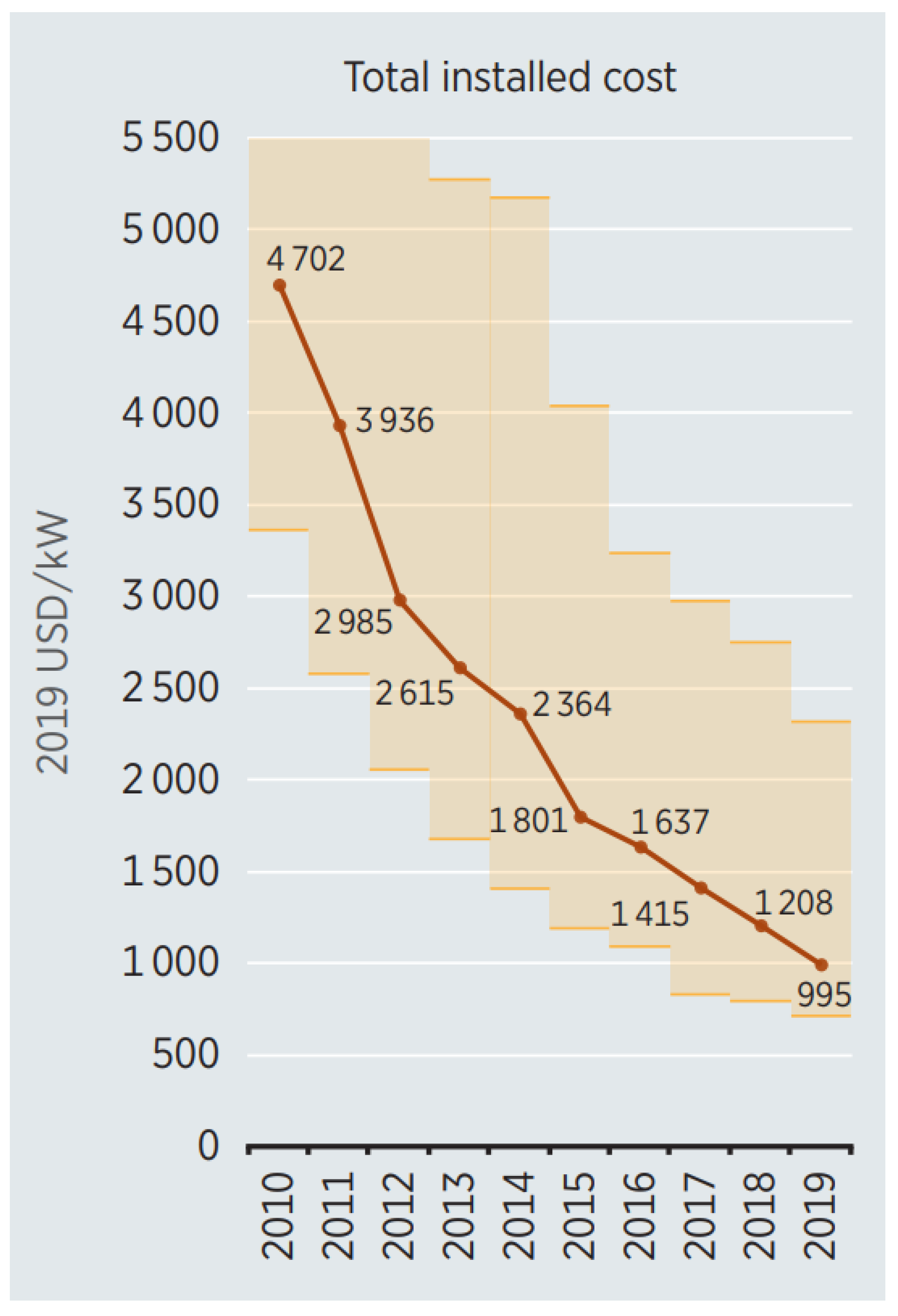
1.2. Economic Evolution of Photovoltaic Energy in the World
1.3. Rooftop Photovoltaic Systems
1.4. Outline of the Article
- Introduction
- 1.1
- Background
- 1.2
- Economic evolution of photovoltaic energy in the world
- 1.3
- Rooftop photovoltaic systems for industrial self-consumption
- 1.4
- Outline of the article
- Materials and methods
- 2.1
- Design and basic engineering of the facilities
- 2.2
- CAPEX calculation
- 2.3
- Simulation of installations with the Helioscope software
- 2.4
- OPEX calculation and estimation of LCOE
- 2.5
- Numerical modeling of the LCOE
- Results and discussion
- 3.1
- Installable power analysis
- 3.2
- Yield analysis
- 3.3
- CAPEX analysis
- 3.4
- LCOE analysis
- Procedure developed for the LCOE calculation
- 4.1
- Procedure compilation
- 4.2
- Accuracy of the developed models
- Conclusions, limitations of the study, and future research
- 5.1
- Conclusions
- 5.2
- Limitations of the study and future research
References
2. Materials and Methods
- Facilities located in Spain: to avoid that different weather conditions or the variation in costs from one country to another may distort the comparison.
- Industrial self-consumption facilities: since the decentralization of the electrical system and the low return on investment generated by these facilities make the installation forecasts very high [24].
- Installations on a flat roof with high tolerance to loads
- Installations with 100% self-consumption: that is, the study is carried out for installations that take advantage of all the energy they generate because their consumption is much higher at all times than photovoltaic production.
- Inverters located in the room of the General Low Voltage Module.
- Absence of obstacles.
- Absence of losses due to close shading.
- Building height of 10 m.
- Selection of standard cases: the variables that will change from one case to another will be defined to represent as many facilities as possible so that conclusions can be drawn on how they affect the different parameters studied.
- Selection of main equipment: the modules, inverters, and structures to be used will be chosen. It will represent the latest advances in the sector, using modules improved by PERC type treatments, multi MPPT inverters, and structures without the need to drill the roof.
- Use the Helioscope software to calculate the available power: the selected geometries will be generated in Helioscope, and the sizing of each of the facilities defined in step 1 will be carried out. Helioscope software has similar error ranges that other PV simulation software, while its interface facilitates making 3D simulations for the defined base cases [25].
- Design and basic engineering of the facilities: to subsequently assess the cost of the plants, the wiring, protections, control equipment, and all the necessary elements for each of the predefined facilities will be dimensioned, always from the point of view of basic engineering. The design has been made according to the Spanish legislation [26].
- Calculation of CAPEX: Each facility will be economically valued, budgeting with market prices for materials and assembly. The cost of engineering, business structure costs, and any other element that may intervene in the budget of a photovoltaic installation will also be calculated.
- Simulation of the installations with the Helioscope software: once the photovoltaic plants have been dimensioned, the data input into Helioscope will be completed. They will be simulated for each of the selected locations, compiling the results obtained.
- Calculation of OPEX and estimation of LCOE: the cost of maintenance will be economically valued. The calculated values of the LCOE for each case can be obtained in the locations studied.
- Numerical modeling of the LCOE: numerical models will be generated that allow an approximate calculation of the power, production, cost, and LCOE of a photovoltaic installation for a known roof.
2.1. Design and Basic Engineering of the Facilities
2.2. CAPEX Calculation
2.3. Simulation of Installations with the Helioscope Software
2.4. OPEX Calculation and Estimation of LCOE
2.4.1. OPEX Calculation
2.4.2. LCOE Calculation
- CAPEX: the cost of the photovoltaic plant in absolute terms. It is obtained from the price of the EPC by adding a 4% surcharge for license taxes in Spain [30].
- OPEX: the cost of annual maintenance in absolute terms, approximated according to the NREL at 1% of CAPEX (considering that maintenance does not imply an expense in building licenses).
- Production year 1: values extracted from the simulation carried out.
- r: discount rate. As it is a facility intended for self-consumption, this value is quite high since the risk associated with a location change, a decrease in consumption, or other problems related to the company’s future that owns the facility is high. A value of 6% will be used, which is between 4 and 8% recommended by Solar Bankability [31] and coincides with the NREL’s recommended values [27].
- a: loss of annual performance of the modules. The 0.7% guaranteed by the manufacturer in the characteristics of the equipment will be used. Those values are aligned with academic research on this topic [32].
- n: useful life of the plant will be considered 30 years [33].
2.5. Numerical Modeling of the LCOE
- Peak power of the installation:
- 2.
- Yield of the installation:
- 3.
- Installation CAPEX and OPEX
- 4.
- LCOE of the installation:
2.5.1. Numerical Modeling of Peak Power
2.5.2. Numerical Modeling of YIELD
2.5.3. Numerical Modeling of CAPEX and OPEX
2.5.4. Numerical Modeling of the LCOE
3. Results and Discussion
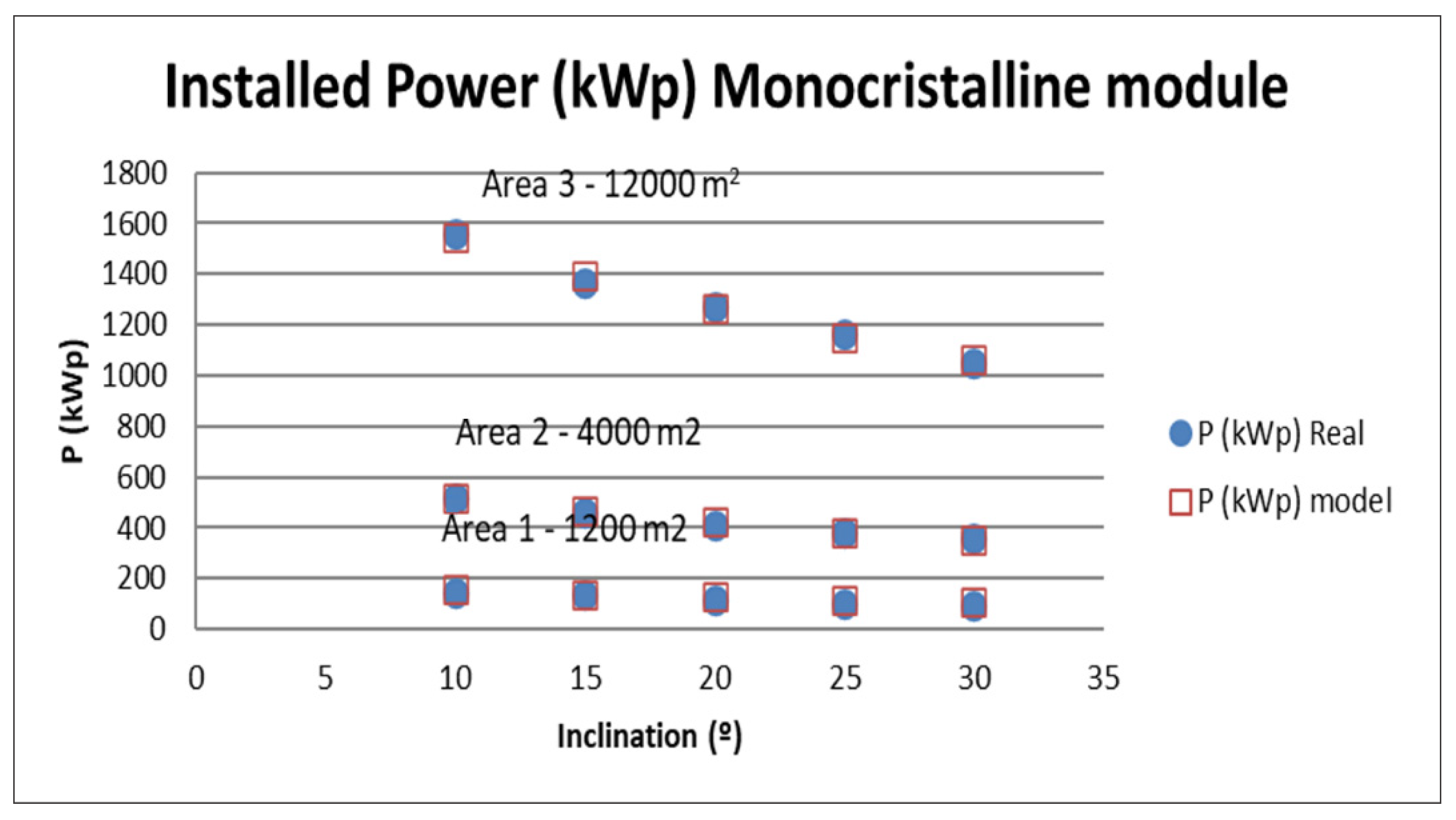
3.1. Installable Power Analysis
3.2. Yield Analysis
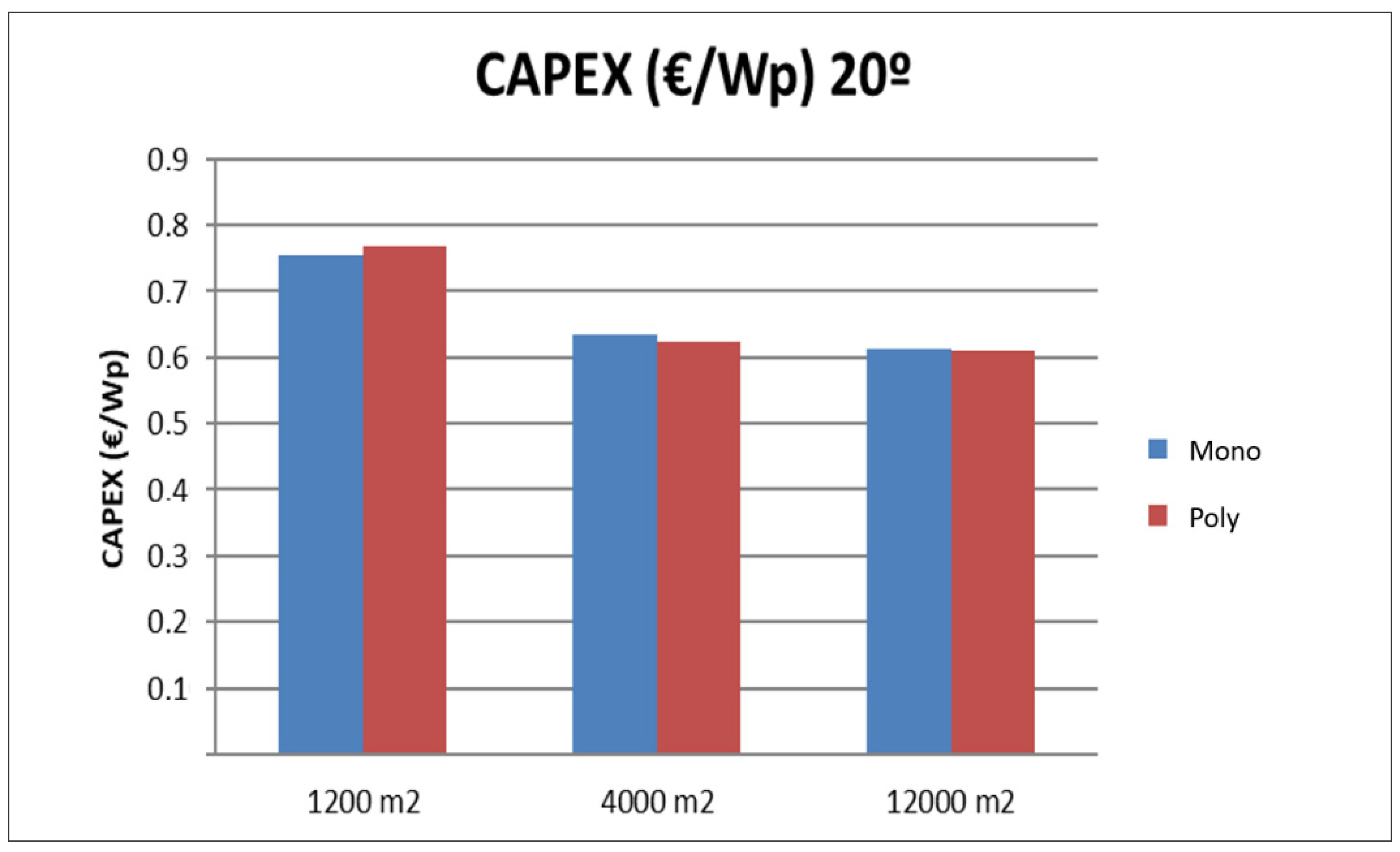
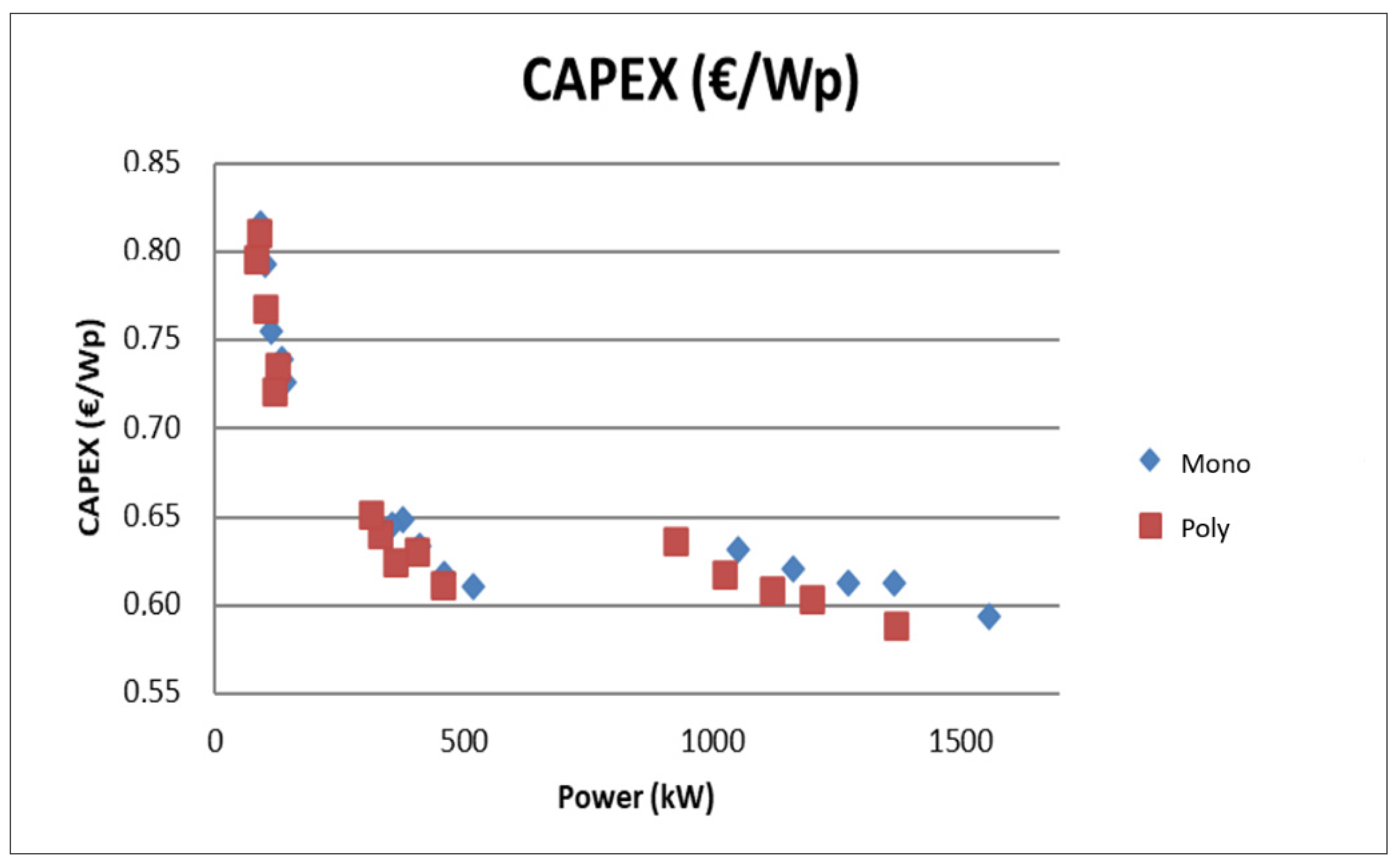
3.3. CAPEX Analysis
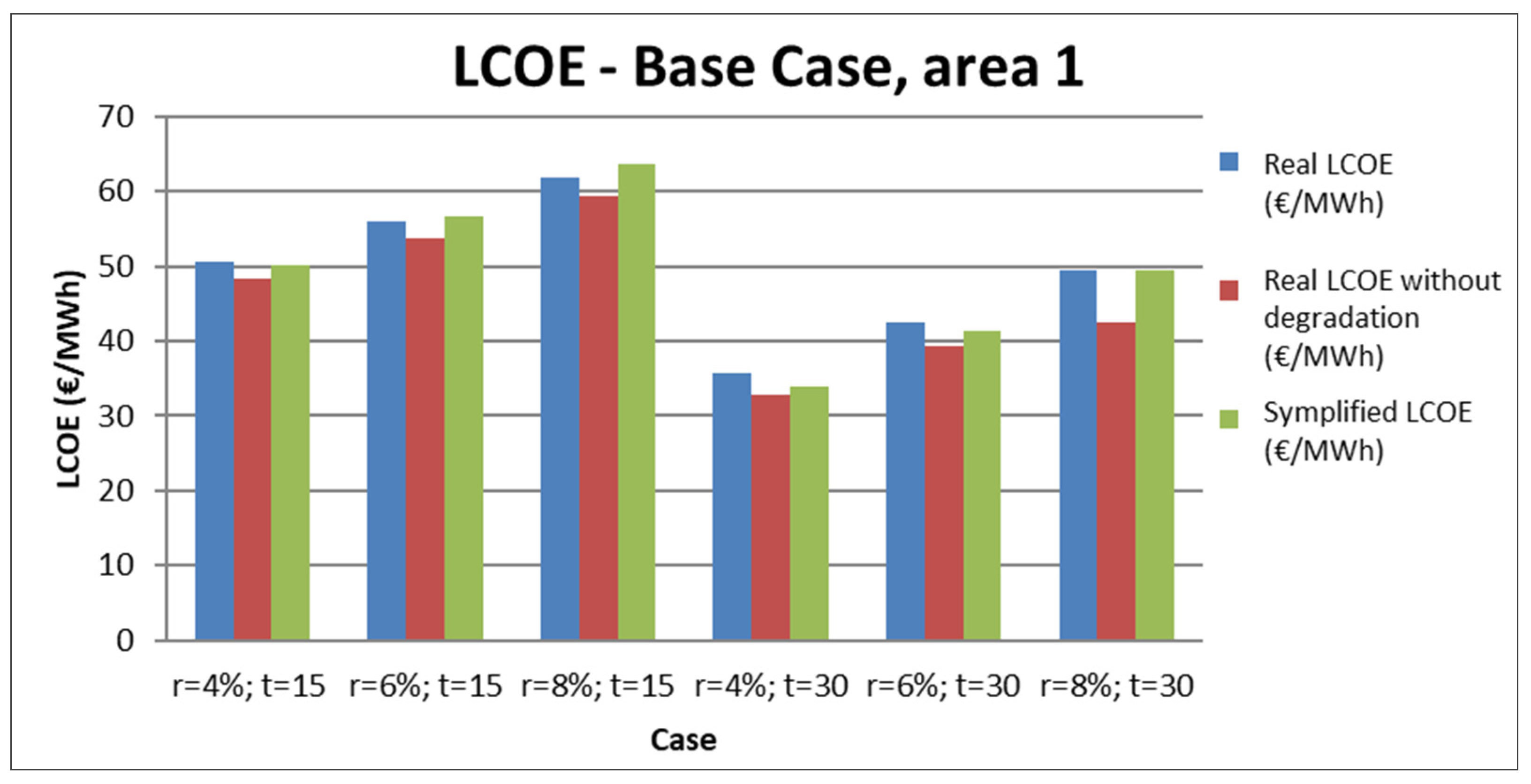
3.4. LCOE Analysis
4. Procedure Developed for the LCOE Calculation
4.1. Procedure Compilation
4.2. Accuracy of the Developed Models
5. Conclusions, Limitations of the Study and Future Research
5.1. Conclusions
5.2. Limitations of the Study and Future Research
Author Contributions
Funding
Data Availability Statement
Conflicts of Interest
Abbreviations
| AC | Alternating Current |
| BIPV | Building Integrated PV |
| CAPEX | Capital Expenditures |
| CRF | Capital Recovery Factor |
| DC | Direct Current |
| DDP | Delivered Duty Paid |
| EPC | Engineering, Procurement, and Construction |
| G | Radiation value in kWp/m2 |
| GHI | Global Horizontal Irradiation |
| GM | Gross Margin |
| HV | Cost of the voltage raising system |
| IEA | International Energy Agency |
| IRENA | International Renewable Energy Agency |
| LCOE | Levelized Cost of Electricity |
| LID | Light Induced Degradation |
| LV | Low Voltage |
| MV | Medium Voltage |
| MPPT | Maximum Power Point Tracker |
| NREL | National Renewable Energy Laboratory |
| OPEX | Operational Expenditures |
| PERC | Passivated Emitter Real Cell |
| PPA | Power Purchase Agreement |
| PR | Performance Ratio |
| PV | Photo-voltaic |
| STC | Standard Test Conditions |
| TS | Transforming Station |
References
- International Energy Agency (IEA). World Energy Outlook 2021, October 2021. Available online: www.iea.org/weo (accessed on 13 October 2021).
- Kavlak, G.; McNerney, J.; Trancik, J.E. Evaluating the causes of the cost reduction in photovoltaic modules. Energy Policy 2018, 123, 700–710. [Google Scholar] [CrossRef] [Green Version]
- International Renewable Energy Agency (IRENA). Renewable Power Generation Costs in 2020. Available online: https://www.irena.org/-/media/Files/IRENA/Agency/Publication/2020/Jun/IRENA_Power_Generation_Costs_2019.pdf (accessed on 13 June 2021).
- Unión Nacional Española de Fotovoltaica (UNEF). Informe Anual de 2018. 2017: El Inicio de una Nueva Era en el Sector Fotovoltaico. Available online: https://unef.es/wp-content/uploads/dlm_uploads/2018/09/memo_unef_2017.pdf (accessed on 18 July 2019).
- Pikerel, K. Latest Lazard LCOE Analysis Finds Utility-Scale Solar Now at or below Cost of Conventional Generation. Available online: https://www.solarpowerworldonline.com/2018/11/latest-lazard-lcoe-analysis-finds-utility-scale-solar-now-at-or-below-cost-of-conventional-generation/ (accessed on 18 July 2019).
- Willuhn, M. La Subasta Portuguesa Bate Record Mundial con 14,8 €/MWh. PV Magazine. Available online: https://www.pv-magazine.es/2019/07/31/la-subasta-portuguesa-bate-el-record-mundial-con-148-e-mwh/ (accessed on 3 August 2019).
- International Energy Agency (IEA). Statistic Data Browsers. Available online: https://www.iea.org/statistics/ (accessed on 13 June 2021).
- Renewable Energy Policy Network for the 21st Century (REN21). Renewables 2016, Global Status Report. Available online: https://www.ren21.net/wp-content/uploads/2019/05/REN21_GSR2016_FullReport_en_11.pdf (accessed on 18 July 2019).
- International Energy Agency-Photovoltaic Power Systems Programme (IEA-PPSP). A Snapshot of Global Photovoltaics. Available online: http://www.iea-pvps.org/index.php?id=266 (accessed on 18 July 2019).
- IRENA. Statistics, Capacity, and Generation. Available online: https://irena.org/Statistics/View-Data-by-Topic/Capacity-and-Generation/Country-Rankings (accessed on 13 June 2021).
- Odeh, S.; Nguyen, T.H. Assessment Method to Identify the Potential of Rooftop PV Systems in the Residential Districts. Energies 2020, 14, 4240. [Google Scholar] [CrossRef]
- Martinopoulos, G. Are rooftop photovoltaic systems a sustainable solution for Europe? A life cycle impact assessment and cost analysis. Appl. Energy 2020, 257, 114035. [Google Scholar] [CrossRef]
- Talavera, D.L.; Muñoz-Rodríguez, F.J.; Jimenez-Castillo, G.; Rus-Casas, C.A. New approach to sizing the photovoltaic generator in self-consumption systems based on cost–competitiveness, maximizing direct self-consumption. Renew. Energy 2019, 130, 1021–1035. [Google Scholar] [CrossRef]
- IEA. Unlocking the Economic Potential of Rooftop Solar in India. 12 October 2020. Workshop. Available online: https://www.iea.org/events/unlocking-the-economic-potential-of-rooftop-solar-in-india (accessed on 23 June 2021).
- IRENA. Renewable Energy Benefits: Leveraging Local Capacity for Solar PV; International Renewable Energy Agency: Abu Dhabi, United Arab Emirates, 2017. [Google Scholar]
- Wang, D.D.; Sueyoshi, T. Assessment of large commercial rooftop photovoltaic system installations: Evidence from California. Appl. Energy 2017, 188, 45–55. [Google Scholar] [CrossRef]
- Department of Energy (USDOE). DOE Releases Solar Futures Study Providing the Blueprint for a Zero-Carbon Grid. October 2021. Available online: https://www.energy.gov/articles/doe-releases-solar-futures-s (accessed on 11 October 2021).
- Zhao, X.; Xie, Y. The economic performance of industrial and commercial rooftop photovoltaic in China. Energy 2019, 187, 115961. [Google Scholar]
- Jara, P.G.B.; Castro, M.T.; Esparcia, E.A., Jr.; Ocon, J.D. Quantifying the Techno-Economic Potential of Grid-Tied Rooftop Solar Photovoltaics in the Philippine Industrial Sector. Energies 2020, 13, 5070. [Google Scholar] [CrossRef]
- Bernasconi, D.; Guariso, G. Rooftop PV: Potential and Impacts in a Complex Territory. Energies 2021, 14, 3687. [Google Scholar] [CrossRef]
- Javeed, I.; Khezri, R.; Mahmoudi, A.; Yazdani, A.; Shafiullah, G.M. Optimal Sizing of Rooftop PV and Battery Storage for Grid-Connected Houses Considering Flat and Time-of-Use Electricity Rates. Energies 2021, 14, 3520. [Google Scholar] [CrossRef]
- Gholami, H.; Nils Røstvik, H. Levelised Cost of Electricity (LCOE) of Building Integrated Photovoltaics (BIPV) in Europe, Rational Feed-In Tariffs and Subsidies. Energies 2021, 14, 2531. [Google Scholar] [CrossRef]
- Bevilacqua, P.; Perrella, S.; Cirone, D.; Bruno, R.; Arcuri, N. Efficiency Improvement of Photovoltaic Modules via Back Surface Cooling. Energies 2021, 14, 895. [Google Scholar] [CrossRef]
- Jäger-Waldau, A. PV Status Report 2019; EUR 29938 EN; Publications Office of the European Union: Luxembourg, 2019; ISBN 978-92-76-12608-9. [Google Scholar] [CrossRef]
- Guittet, D.L.; Janine, M.F. Validation of Photovoltaic Modeling Tool HelioScope Against Measured Data; NREL/TP-6A20-72155; National Renewable Energy Laboratory: Golden, CO, USA. Available online: https://www.nrel.gov/docs/fy19osti/72155.pdf (accessed on 26 September 2021).
- Bueno, B. Reglamento Electrotécnico de Baja Tensión, 4th ed.; Marcombo: Barcelona, Spain, 2018; ISBN 978-84-267-2562-2. [Google Scholar]
- National Renewable Energy Laboratory (NREL). Best Practices in Photovoltaic Systems Operation and Maintenance, 2nd ed.; NREL: Golden, CO, USA, 2016. Available online: https://www.nrel.gov/docs/fy17osti/67553.pdf (accessed on 12 July 2019).
- Lindroos, J.; Savin, H. Review of Light-Induced Degradation in Crystalline Silicon Solar Cells. Sol. Energy Mater. Sol. Cells 2016, 147, 115–126. [Google Scholar] [CrossRef]
- Electric Power Research Institute (EPRI). Budgeting for Solar Plants O&M: Practices and Pricing. 2015. Available online: https://prod-ng.sandia.gov/techlib-noauth/access-control.cgi/2016/160649r.pdf (accessed on 23 July 2019).
- State Gazette; Boletín Oficial del Estado. Real Decreto Legislativo 2/2004 de 5 de Marzo, Por el Que se Aprueba el Texto Refundido de la Ley Reguladora de las Haciendas Locales. BOE 59, 13 July 2004. Available online: https://www.boe.es/buscar/act.php?id=BOE-A-2004-4214 (accessed on 9 October 2021). (In Spanish)
- Solar Bankability. Best Practice Guidelines for PV Cost Calculation, Accounting for Technical Risks and Assumptions in PV LCOE. Available online: https://www.tuv.com/content-media-files/master-content/services/products/p06-solar/solar-downloadpage/solar-bankability_d3.2_best-practice-guidelines-for-pv-cost-calculation.pdf (accessed on 30 June 2019).
- Ishii, T.; Masuda, A. Annual degradation rates of recent crystalline silicon photovoltaic modules. Prog. Photovolt. 2017, 25, 953–967. [Google Scholar] [CrossRef]
- Muhleisen, W. Scientific and economic comparison of outdoor characterization methods for photovoltaic power plants. Renew. Energy 2019, 134, 321–329. [Google Scholar] [CrossRef]
- Good, J.; Johnson, J. Impact of inverter loading ratio on solar photovoltaic system performance. Appl. Energy 2017, 177, 475–486. [Google Scholar]
- Mermoud, A. PVSYST User’s Manual; PVSYST SA: Satigny, Switzerland, 2014. [Google Scholar]
- National Renewable Energy Laboratory (NREL). Crystalline Silicon Photovoltaic Module Manufacturing Costs and Sustainable Pricing: 1H 2018 Benchmark and Cost Reduction Road Map. Available online: https://www.nrel.gov/docs/fy19osti/72134.pdf (accessed on 25 September 2021).
- National Renewable Energy Laboratory (NREL). Simple Levelized Cost of Energy Calculator Documentation. Available online: https://www.nrel.gov/analysis/tech-lcoe-documentation.html (accessed on 30 July 2019).
- Short, J. A Manual for the Economic Evaluation of Energy Efficiency and Renewable Energy Technologies; NREL: Golden, CO, USA, 1995. [Google Scholar]
- Meteoblue Climate (Modeled). Available online: https://www.meteoblue.com/es/tiempo/historyclimate/climatemodelled/sevilla_espa%c3%b1a_2510911 (accessed on 6 August 2019).
- ADRASE (Acceso a Datos de Radiación Solar en España). Mapa Interactivo de la Península. Available online: http://www.adrase.com/ (accessed on 28 July 2019).
- National Renewable Energy Laboratory (NREL). US Solar Photovoltaic Systems Cost Benchmark: Q1 2017; NREL: Golden, CO, USA, 2017.
- State Gazette. Royal Decree 244/2019, of April 5, Which Regulates the Administrative, Technical and Economic Conditions of the Self-Consumption of Electrical Energy; Reference: BOE-A-2019-5089; Boletín Oficial del Estado (State Gazette): Madrid, Spain. Available online: https://www.boe.es/eli/es/rd/2019/04/05/244 (accessed on 26 September 2021). (In Spanish)
- Gatto, A.; Drago, C. When renewable energy, empowerment, and entrepreneurship connect: Measuring energy policy effectiveness in 230 countries. Energy Res. Soc. Sci. 2021, 78, 101977. [Google Scholar] [CrossRef]
- Żuk, P.; Żuk, P. Increasing Energy Prices as a Stimulus for Entrepreneurship in Renewable Energies: Ownership Structure, Company Size and Energy Policy in Companies in Poland. Energies 2021, 14, 5885. [Google Scholar] [CrossRef]
- Aldieri, L.; Barra, C.; Ruggiero, N.; Vinci, C.P. Green Energies, Employment, and Institutional Quality: Some Evidence for the OECD. Sustainability 2021, 13, 3252. [Google Scholar] [CrossRef]


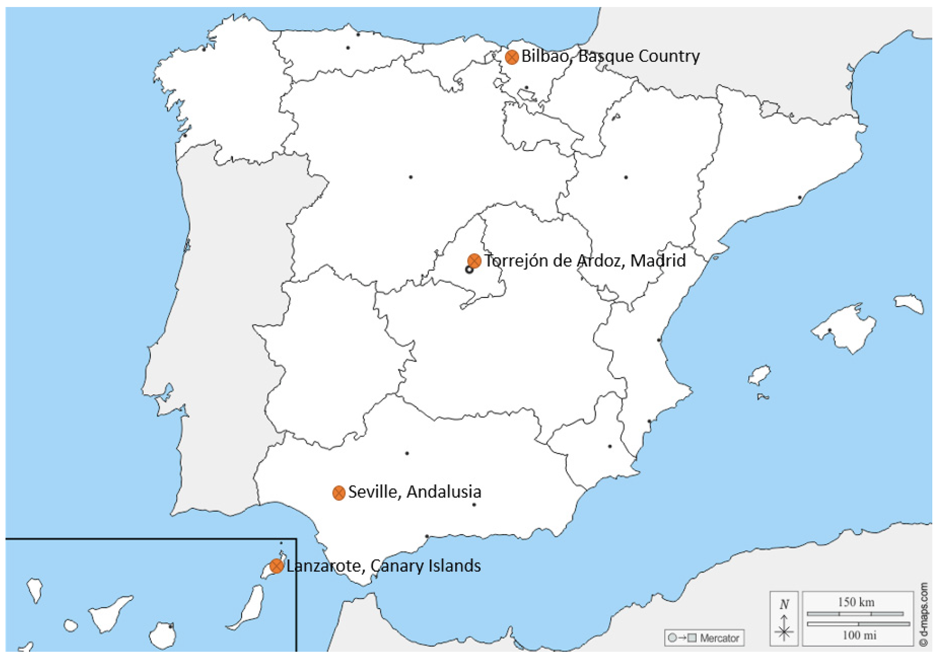
| Location | Latitude | Longitude |
|---|---|---|
| Bilbao, Basque Country | 43° 14′ N | 2° 55′ W |
| Torrejón de Ardoz, Madrid | 40° 26′ N | 3° 38′ W |
| Seville, Andalusia | 37° 22′ N | 5° 59′ W |
| Lanzarote, Canary Islands | 28° 58′ N | 13° 32′ W |
| Element | 10°-Mono-1200 Cost (€) | 10°-Mono-4000 Cost (€) | 10°-Mono-12,000 Cost (€) |
|---|---|---|---|
| Photovoltaic Modules | 41,325 | 143,034 | 413,201 |
| Structures | 7524 | 27,462 | 77,754 |
| Investors and add-ons | 9470 | 25,413 | 64,037 |
| DC wiring | 1811 | 8900 | 42,351 |
| AC wiring (LV and MV) | 985 | 2139 | 59,436 |
| Protections and control | 4686 | 12,480 | 17,470 |
| Mounting | 11,472 | 36,647 | 108,428 |
| Structure of work | 12,916 | 22,176 | 29,918 |
| Miscellaneous expenses | 2233 | 5430 | 14,514 |
| Cost | 92,425 | 283,685 | 827,112 |
| Margin | 11,091 | 34,042 | 99,253 |
| Sale | 103,516 | 317,727 | 926,366 |
| Element | 10°-Mono-1200 | 10°-Mono-4000 | 10°-Mono-12,000 |
|---|---|---|---|
| EPC (€) | 103,516 | 317,727 | 926,366 |
| Power (kWp) | 142.5 | 520.1 | 1559.3 |
| EPC (€/Wp) | 0.726 | 0.611 | 0.594 |
| Parameter | 10°-Mono-1200 | 10°-Mono-4000 | 10°-Mono-12,000 |
|---|---|---|---|
| PR (%) | 84.9 | 84.5 | 84.7 |
| Yield (kWh/kWp) | 1548 | 1540.5 | 1544.5 |
| Production (MWh/year) | 220.6 | 801.2 | 1408 |
| Case | Module (€/Wp) | Inverter (€/Wp) | Structure (€/Wp) | Assembly (€/Wp) | Other (€/Wp) |
|---|---|---|---|---|---|
| 1200 m2—Mono | 0.290 | 0.063 | 0.086 | 0.086 | 0.231 |
| 1200 m2—Poly | 0.250 | 0.072 | 0.097 | 0.097 | 0.251 |
| 4000 m2—Mono | 0.275 | 0.053 | 0.073 | 0.073 | 0.159 |
| 4000 m2—Poly | 0.240 | 0.050 | 0.083 | 0.083 | 0.169 |
| 12,000 m2—Mono | 0.265 | 0.042 | 0.072 | 0.072 | 0.163 |
| 12,000 m2—Poly | 0.230 | 0.043 | 0.081 | 0.081 | 0.174 |
| Module | Dimensions (mm × mm) | |
|---|---|---|
| 320 Wp, polycrystalline | 1960 × 992 | 16.5 |
| 325 Wp, polycrystalline | 1960 × 992 | 16.7 |
| 330 Wp, polycrystalline | 1960 × 992 | 16.9 |
| 370 Wp, monocrystalline | 1960 × 992 | 19.0 |
| 375 Wp, monocrystalline | 1960 × 992 | 19.3 |
| Module | 330 Wp/Polycrystalline | 375 Wp/Monocrystalline |
|---|---|---|
| 75 kWp–250 kWp | 0.25 | 0.29 |
| 250 kWp–750 kWp | 0.24 | 0.28 |
| 750 kWp–2500 kWp | 0.23 | 0.27 |
| Power | Cost (€/Wp) |
|---|---|
| 75 kWp–250 kWp | 0.070 |
| 250 kWp–750 kWp | 0.055 |
| 750 kWp–2500 kWp | 0.045 |
| Power | Counterweight, 330 Wp Module | Counterweight, 375 Wp Module | Battens, 330 Wp Module | Battens, 375 Wp Module |
|---|---|---|---|---|
| 75kWp–750 kWp | 0.060 | 0.053 | 0.121 | 0.106 |
| 750kWp–2500 kWp | 0.057 | 0.05 | 0.115 | 0.101 |
| Case | Model Error–Other Costs | Model Error—CAPEX |
|---|---|---|
| 10°-Mono-1200 | 5.01% | 3.92% |
| 10°-Mono-4000 | 6.51% | 5.61% |
| 10°-Mono-12,000 | 2.22% | 2.61% |
| r (%) | Years | Relative Error (%) |
|---|---|---|
| 4 | 15 | 0.95 |
| 6 | 15 | 1.09 |
| 8 | 15 | 3.16 |
| 4 | 30 | 5.01 |
| 6 | 30 | 2.33 |
| 8 | 30 | 0.26 |
Publisher’s Note: MDPI stays neutral with regard to jurisdictional claims in published maps and institutional affiliations. |
© 2021 by the authors. Licensee MDPI, Basel, Switzerland. This article is an open access article distributed under the terms and conditions of the Creative Commons Attribution (CC BY) license (https://creativecommons.org/licenses/by/4.0/).
Share and Cite
Rodríguez-Martinez, Á.; Rodríguez-Monroy, C. Economic Analysis and Modelling of Rooftop Photovoltaic Systems in Spain for Industrial Self-Consumption. Energies 2021, 14, 7307. https://doi.org/10.3390/en14217307
Rodríguez-Martinez Á, Rodríguez-Monroy C. Economic Analysis and Modelling of Rooftop Photovoltaic Systems in Spain for Industrial Self-Consumption. Energies. 2021; 14(21):7307. https://doi.org/10.3390/en14217307
Chicago/Turabian StyleRodríguez-Martinez, Álvaro, and Carlos Rodríguez-Monroy. 2021. "Economic Analysis and Modelling of Rooftop Photovoltaic Systems in Spain for Industrial Self-Consumption" Energies 14, no. 21: 7307. https://doi.org/10.3390/en14217307