Fault-Tolerant Cooperative Control of Large-Scale Wind Farms and Wind Farm Clusters

Abstract

Large-scale wind farms and wind farm clusters with many installed wind turbines are increasingly built around the world, and especially in offshore regions. The reliability and availability of these assets are critically important for cost-effective wind power generation. This requires effective solutions for online fault detection, diagnosis and fault accommodation to improve the overall reliability and availability of wind turbines and entire wind farms. To meet this requirement, this paper proposes a novel active fault-tolerant cooperative control (FTCC) scheme for large-scale wind farms and wind farm clusters (WFCs). The proposed scheme is based on a signal correction method at wind turbine level that is augmented with two innovative “control reallocation” mechanisms at wind farm and network operator levels. Applied to a WFC, this scheme detects, identifies and accommodates the effects of both mild and severe power-loss faults in wind turbines. Various simulation studies on an advanced WFC benchmark indicate the high efficiency and effectiveness of the proposed solutions.

1. Introduction

Wind power generation is booming and will continue to do so for the foreseeable future. Increasingly offshore wind turbines are installed in groups called wind farms, and several wind farms in direct vicinity constitute a wind farm cluster (WFC).

Cost-effective large-scale wind power generation by an offshore WFC is particularly challenging due to the increased complexity of offshore assets, limited accessibility, and harsher environmental loadings, all of which result in soaring rates of faults and failures. Given that, effective solutions for online fault detection and diagnosis (FDD) and fault-tolerant control (FTC) are necessary to enhance reliability and availability of wind turbines and wind farms. According to the technical literature, such solutions can be designed, depending on the type and nature of faults, either at an individual wind turbine level or at an entire wind farm (or even WFC) level.

Reviewing the literature, most of the published papers have studied the applications of FDD and FTC at the wind turbine level (e.g., see [1,2,3,4,5,6,7,8,9]). Conversely, the number of published papers on FDD and FTC at the wind farm level is relatively small. For instance, various data-driven methods are presented in [10,11,12] to develop suitable models for fault detection and prediction in wind farms. In [13,14], different machine learning techniques are used to model and monitor wind farm power curves. Work in [15] employs interval parameter-varying parity equations to achieve fault diagnosis in a wind farm. Furthermore, authors in [16] present an active FTC scheme which uses a model-based FDD system. In [17], the problem of active power control in a wind farm is converted to the rotor speed tracking problem, and an adaptive FTC scheme is presented to track the power signal of each wind turbine with an acceptable transient performance and robustness to the actuator faults. The particle swarm optimization (PSO) approach is used in [18] for optimal active power dispatch in a wind farm during generator cooling system faults. A PSO-based active power dispatch method is introduced in [19] to accommodate the fault effects (i.e., inter-turn short circuit faults in wind turbines generators) at the farm level.

In the case of decreased power production because of blade erosion/debris build-up, different FTC solutions under a cooperative framework, called “fault-tolerant cooperative control (FTCC)” schemes, are presented in [20,21]. Having no dependence on the information of wind speed or direction, the said schemes can simultaneously handle multiple faults in wind turbines of a wind farm with any arbitrary layouts. Badihi et al. in [22] extends the authors’ works in [20,21] by developing another FTCC scheme which relies on an effective “model reference adaptive proportional-integral control reconfiguration” algorithm that is integrated with a “control reallocation” mechanism. Compared with the solutions in [20,21], the more recently developed scheme in [22] can handle both mild and severe power-loss faults because of different levels of icing or debris build-up on wind turbine rotor blades.

Table 1. Examples of existing literature on FDD, FTC, and FTCC of wind farms.

Design Approaches	Objectives	References
Various data-mining-based algorithms	Prediction of wind turbine faults	[10,11]
Principal component analysis	Reducing the dataset for turbine FDD	[12]
Various machine learning methods	Modeling and estimation of a wind farm power curve	[13,14]
Interval nonlinear parameter-varying	Fault diagnosis of a wind farm	[15]
Fuzzy model-based FDD with signal correction	Active FTC for a wind farm against decreased power generation	[16]
Adaptive FTC using barrier Lyapunov function	Active power control during actuator fault	[17]
Particle swarm optimization	Accommodation of the generator fault effects at farm level	[18,19]
FTCC using fuzzy logic at farm level	Accommodation of mild power-loss faults caused by turbine blade erosion and debris build-up on the blades	[20,21]
FTCC using adaptive PI control at turbine level and control reallocation at farm level	Accommodation of mild and severe power loss faults caused by turbine blade erosion and debris build-up on the blades	[22]

presents a categorized list of the references on FDD, FTC, and FTCC of wind farms with their corresponding design approaches.

It should be noted that the effective implementation of the presented scheme in [22] for a large-scale wind farm or WFC, where the number of wind turbines becomes quite large, turns to be complex or computationally expensive due to the increased number of modules required in the scheme (i.e., each module monitors the power consistency between two different turbines in the wind farm). To overcome these issues when dealing with very large-scale wind farms or WFCs, the present paper proposes a novel clustering approach to enable a computationally efficient multilayer FTCC scheme which provides effective fault identification and accommodation performance with simplified computer programming. For this purpose, it is reasonable to suppose that a very large-scale wind farm or WFC can be divided into a group of smaller scale wind farms, each including a smaller number of wind turbines. In other words, a very large-scale wind farm can be studied as a WFC consisting of several smaller wind farms that are directly/indirectly connected to a node of transmission network. In the presented scheme, a distributed FDD system is applied on each smaller wind farm in the cluster that reduces the total number of computational modules. Accordingly, a multilayer FTCC scheme is designed and implemented at three control levels (i.e., turbine, farm, and cluster levels) to accommodate mild and severe power-loss faults in any wind turbine. The mild power-loss faults are accommodated at a primary control level (turbine level) using a signal correction approach, while the secondary and tertiary control levels (farm and cluster levels, respectively) are used for accommodating severe power-loss faults. In this regard, control reallocation mechanisms for each smaller wind farm, and also the network operator, are introduced. Various simulation studies on an advanced WFC benchmark, including 100 wind turbines, reveals the notable effectiveness of the proposed solutions in the presence of realistic fault scenarios, as well as wind turbulences and measurement noises.

The remainder of this paper is ordered as follow. The WFC benchmark as well as the considered faults are discussed in Section 2. Section 3 presents the proposed FTCC scheme to tackle the faults in Section 2. Section 4 illustrates and discusses the obtained simulation results. Finally, Section 5 draws some important conclusions and proposes future work.

2. WFC Benchmark and Power-Loss Faults

Using the “SimWindFarm” toolbox in [23], an advanced dynamic simulation model was developed to represent a WFC benchmark. The original toolbox created a nonlinear wind farm model that allows studying wind farm controls and diagnostics in the presence of realistic operating conditions. This paper considers WFC $Q$ that includes $N$ wind farms each of which referred to as $Q_i$ consisting of $N_i$ wind turbines. In other words, WFC $Q$ with $N$ wind farms is represented as $Q=\left\{Q_i|i\in \mathbb{N}, i\le N\right\}$ and wind farm $Q_i$ with $N_i$ turbines is represented as $Q_i=\left\{q_j|j\in \mathbb{N},j\le N_i\right\}$ (Note: $\mathbb{N}$ is the set of natural numbers, and $q_j$ is the $j$th turbine in wind farm $Q_i$). The considered layout of a WFC with 100 wind turbines (i.e., ten wind farms, each having ten 5-MW wind turbines), and the benchmark block diagram under consideration are illustrated in Figure 1 and Figure 2, respectively.

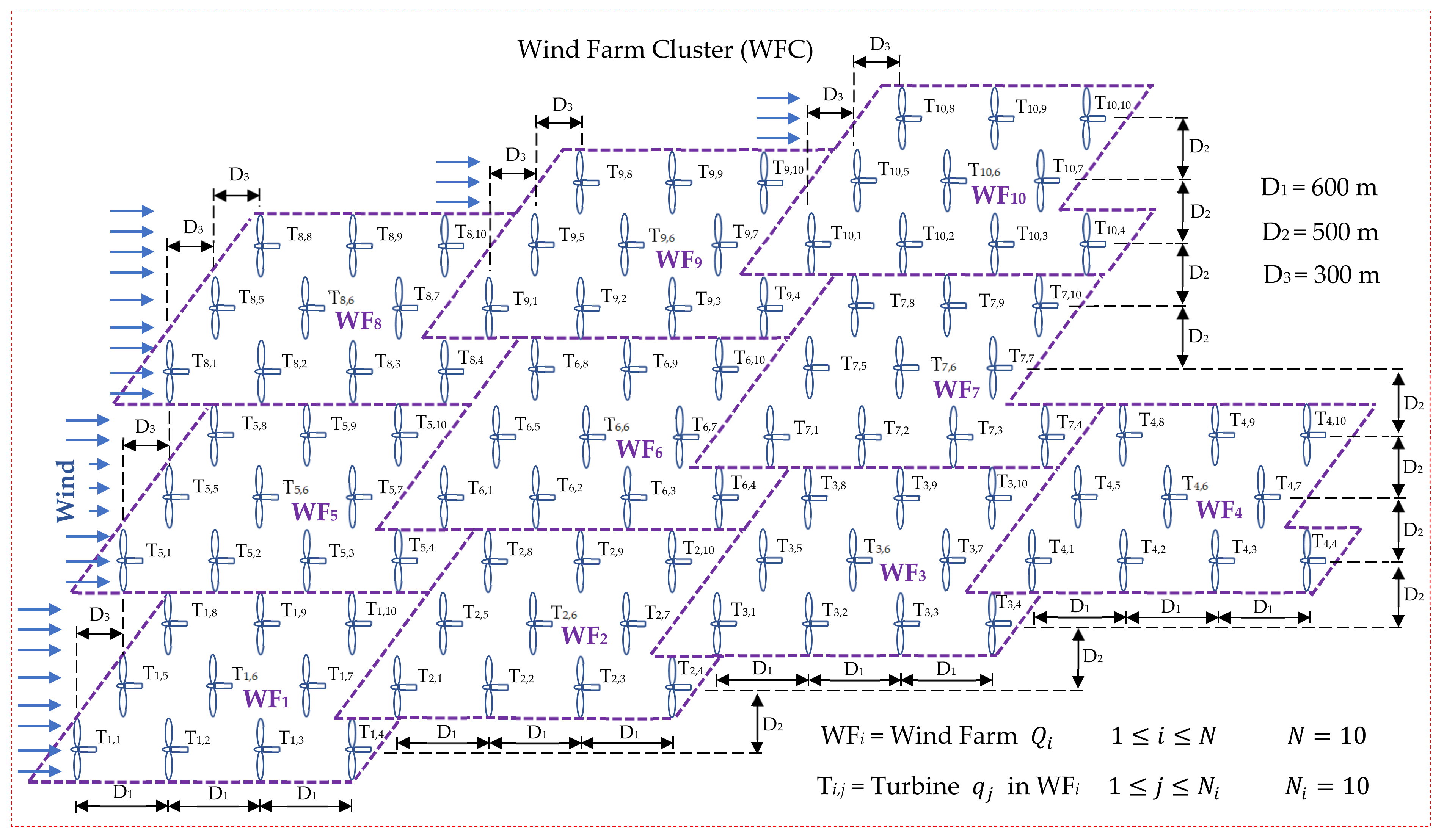
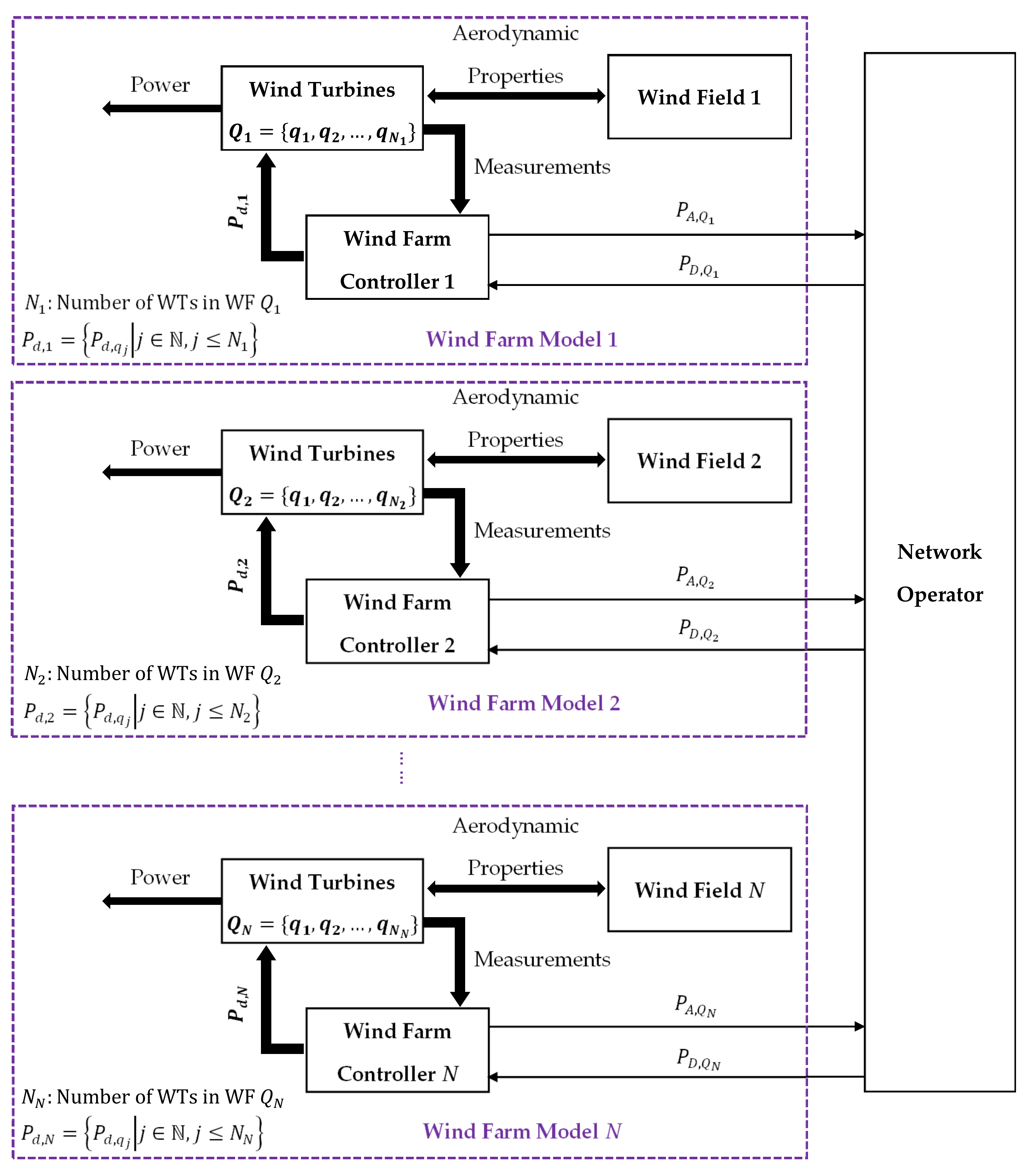
2.1. Benchmark Components

As shown in Figure 2, there are four major components in the benchmark model, namely the “wind farm controller”, “wind turbines” and “wind field” for each wind farm in WFC, and the “network operator”. The following paragraphs provide more information about these components:

Network Operator: This component relates to the tertiary control level and can work in different operational modes such as “absolute”, “delta”, or “frequency regulation” to specify the “total demanded active power” $P_D$ of the WFC $Q$ (i.e., $P_D={{\displaystyle \sum }}_{i=1}^N{P}_{D,Q_i}$ where $P_{D,Q_i}$ is the demanded power of wind farm $Q_i$ in the cluster) required for reliable connection of the WFC to the power grid. Among the above-mentioned operational modes, this paper employs the “frequency regulation mode”, using which the measured grid frequency$f_{mes}$ is considered as a feedback signal to enable online “active power control (APC)”. The aim of APC is to maintain the essential balance between generated power in WFC and demanded power by grid load, which thus regulates the frequency to its reference value$f_r$, despite a changing load. The baseline network operator in frequency regulation mode includes a “dead-band proportional gain control” that uses the frequency error $f_e$ in Equation (1) to compute $P_D$ at the time-step ($k+1$) from Equation (2). Such a simple control system regulates the frequency to any specified reference value; for example, 50 Hz that is commonly used in large areas of the world [21].

$$f_e\left(k\right)=f_{mes}\left(k\right)-f_r$$

(1)

$$P_D\left(k+1\right)=\left\{\begin{array}{cc}{P}_{min}\hfill & \hfill f_e\left(k\right)\ge c\\ \frac{P_{max}+P_{min}}{2}-\frac{\left(P_{max}-P_{min}\right)\left(f_e\left(k\right)-d\right)}{2\left(c-d\right)}& \hfill d<f_e\left(k\right)<c\\ \frac{P_{max}+P_{min}}{2}\hfill & \hfill -d\le f_e\left(k\right)\le d\\ \frac{P_{max}+P_{min}}{2}-\frac{\left(P_{max}-P_{min}\right)\left(f_e\left(k\right)+d\right)}{2\left(c-d\right)}\hfill & \hfill -c<f_e\left(k\right)<-d\\ P_{max}\hfill & \hfill f_e\left(k\right)\le -c\end{array}\right.$$

(2)

In Equation (2), the constants $c$ and $d$ respectively denote the “control-band” and the “dead-band” values ($c>d$) defined by user. In addition, $P_{min}$ and $P_{max}$ denote the prescribed minimum and maximum limits for the total power produced by the WFC, respectively. Finally, the network operator distributes the WFC’s $P_D$ among wind farms in the cluster via the proportional algorithm in Equation (3).

$$P_{D,Q_i}\left(k+1\right)=P_D\left(k+1\right)\frac{P_{A,Q_i}\left(k\right)}{P_A\left(k\right)}\hspace{1em},\hspace{1em}\hspace{1em}{Q}_i\in Q$$

(3)

where $P_{D,Q_i}$ denotes the demanded power from wind farm $Q_i$ in the WFC $Q$, and $P_{A,Q_i}$ denotes the estimated available power in the same wind farm. $P_A$ is the estimated total available power of the WFC. It is worth noting that the simple control law in Equation (3) is designed for a WFC in which all wind farms are healthy. Otherwise, the network operator’s fault-tolerant control solutions should be considered, as explored in Section 3.4.

Wind Farm Controller: Each wind farm in the cluster has a wind farm controller that corresponds to the secondary control level. The $i$th wind farm controller is an interface between the already-explained network operator and wind turbines in the wind farm $Q_i$. At each $k$ (time-step), it provides the operator with an estimate of the total available power $P_{A,Q_i}$ in the wind farm $Q_i$. In addition, it distributes the wind farm total demanded power $P_{D,Q_i}$ (received from the network operator) among wind turbines based on the proportional algorithm below:

$$P_{d,q_j}\left(k+1\right)=P_{D,Q_i}\left(k+1\right)\frac{P_{a,q_j}\left(k\right)}{P_{A,Q_i}\left(k\right)}\hspace{1em},\hspace{1em}\hspace{1em}{q}_j\in Q_i$$

(4)

where $N_i$ is the number of wind turbines in the wind farm $Q_i$, and $P_{d,q_j}\left(k+1\right)$ denotes the demanded power from wind turbine $q_j$ in the considered wind farm.

Moreover, $P_{a,q_j}\left(k\right)$ denotes the estimated available power in turbine $q_j$ that is obtained by [23]:

$$P_{a,q_j}\left(k\right)=\frac{\pi }{2}\rho R^2{V}_{mes,q_j}{\left(k\right)}^3{C}_{Pmax}$$

(5)

where $\rho$ is the air density, $R$ is the rotor radius, $C_{Pmax}$ is the maximum power coefficient, and $V_{mes,q_j}\left(k\right)$ is the measured nacelle wind speed of wind turbine $q_j$ in the wind farm $Q_i$. Similar to that mentioned for Equation (3), note that the control algorithm in Equation (4) is designed for a healthy wind farm where wind turbines are all healthy with no faults or failures. Otherwise, fault-tolerant wind farm control solutions should be considered as discussed in Section 3.3.

Wind Turbines: This component simulates the real-life dynamics of $N_i$ wind turbines installed in wind farm $Q_i$ using nonlinear models of an offshore 5-MW turbine that is already available by the U.S. National Renewable Energy Laboratory (NREL) [24]. For outputs, the wind turbines component generates the active power along with a set of measurements for use by the wind farm controller. Using a wind turbine control system, each individual wind turbine $q_j$ inside this component acts upon the power demand $P_{d,q_j}$ in Equation (4). The wind turbine control system comprises a blade-pitch controller and a generator torque controller (as primary control level) to compute proper reference values for blade-pitch angle ${\beta }_{r,q_j}$ and generator torque${\tau }_{r,q_j}$, respectively. It is worth noting that the generator torque controller is programed to be active during both below and above rated wind speeds.

Wind Field: Using an appropriate ambient field model along with a wake model, each wind farm has a wind field model that simulates the aerodynamic interactions between wind turbines in the farm.

2.2. Power-Loss Faults

Power-loss faults in wind turbines are highly probable and can be caused by different reasons such as debris build-up or icing on rotor blades [25]. As discussed in [26,27], even mild levels of this type of fault can lead to a substantial off-normal turbine operation and loading and reduced power generation by the wind turbine. If not handled in a timely and effective way, serious problems may arise with optimal tracking of electric grid loads and maintaining a safe frequency at the point of interconnection to the electric grid. Addressed in Section 3, this type of fault can be effectively tackled by implementing a novel FTCC scheme that identifies and accommodates the effects of mild to severe power-loss faults. For wind turbines, wind farms, and the entire WFC, this scheme improves reliability and availability while lowering operation and maintenance costs.

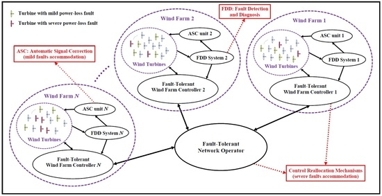
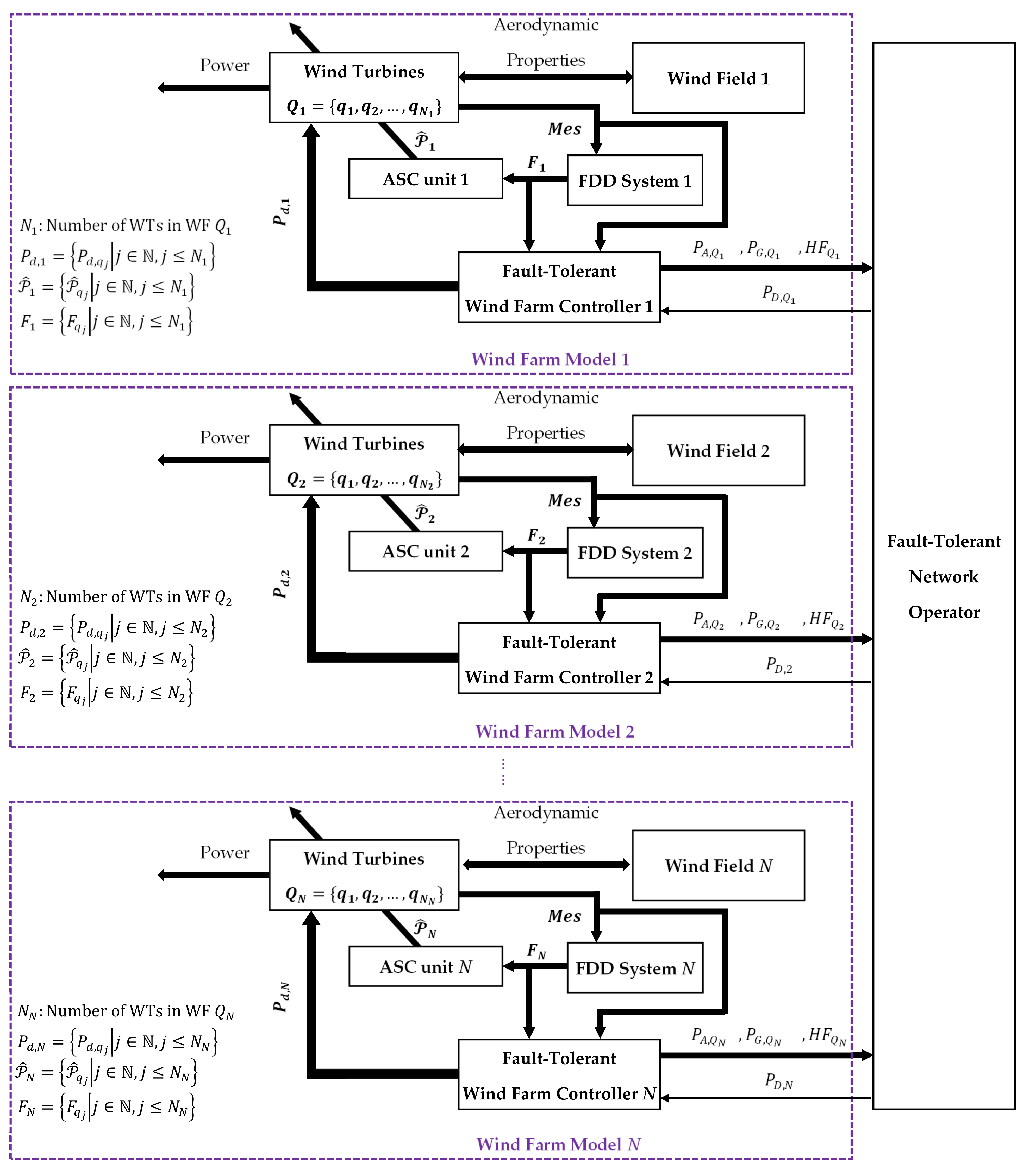
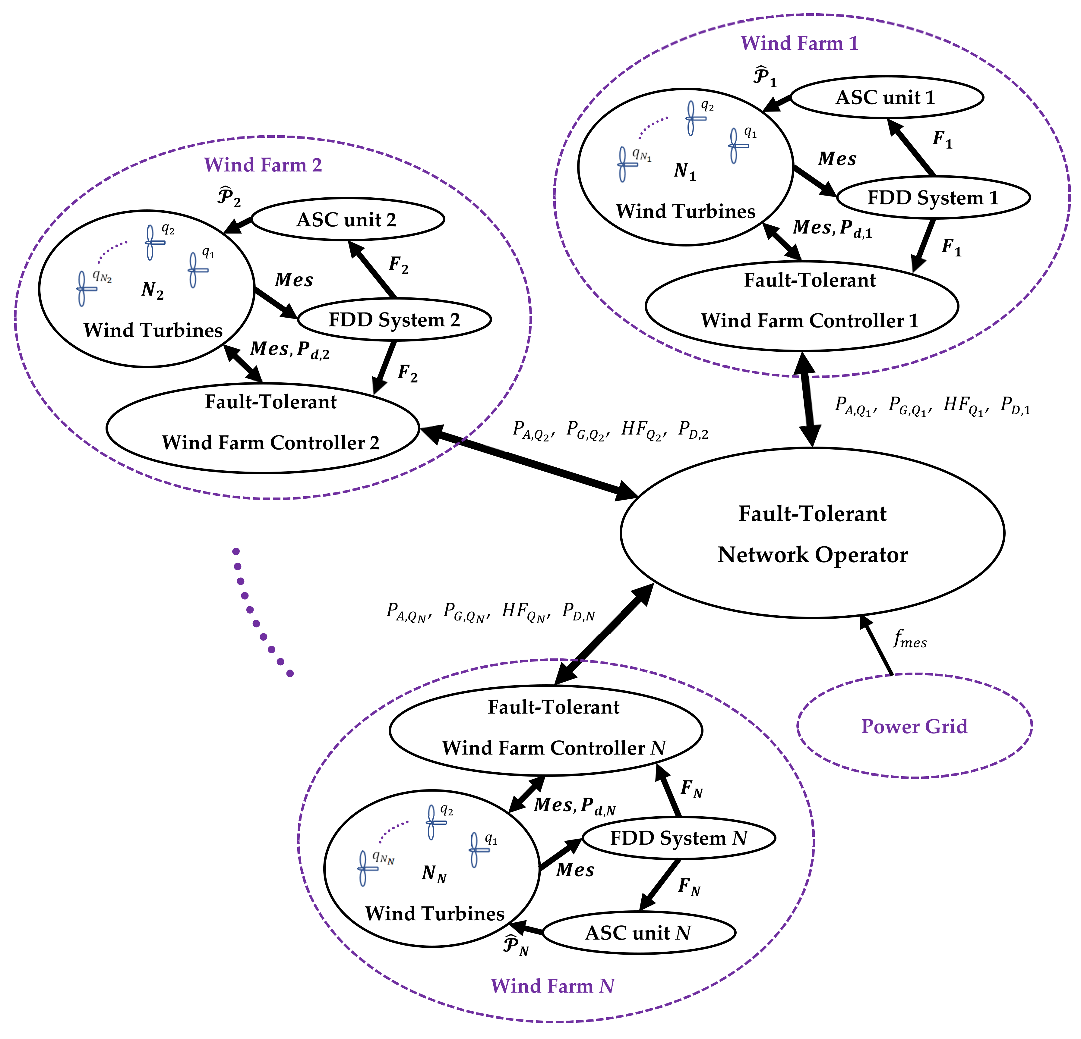
3. Active FTCC Design

This section presents a novel active FTCC scheme based on a signal correction approach at wind turbine (or primary control) level that is augmented with two innovative control reallocation mechanisms at the wind farm (or secondary control) and WFC (or tertiary control) levels. The differences between active and passive fault-tolerant methods are explained in several papers [28,29,30]. In summary, compared with passive approaches, active strategies rely on diagnosis information from an FDD system to deal with a larger variety of faults. As shown in Figure 3, this cooperative framework covers the entire WFC, regardless of wind directions and layouts. The architecture of the proposed FTCC scheme with communication links between different components in the WFC is illustrated in Figure 4.

Similar to the works in [20,21,22], the basic idea for designing an FDD system is to monitor and analyze the consistency of the generated powers from wind turbines altogether in real time. However, in contrast to the above-cited works, the proposed scheme in this paper acts against both mild and severe power-loss faults while using distributed FDD systems, which operate in parallel to detect and identify power-loss faults in each wind farm in a cluster. Indeed, the FDD process is separately carried out at each small-scale wind farm inside a WFC so that each wind farm includes its own FDD system working in parallel with the rest of FDD systems in other wind farms and is responsible for detection and identification of mild and severe faults in the relevant wind farm.

As shown in Figure 3 and Figure 4, the active FTCC scheme includes $N$ FDD systems, $N$ automatic signal correction (ASC) units, $N$ fault-tolerant controllers, and one fault-tolerant network operator, all of which work together to identify the power-loss faults and accommodate the adverse impacts of faults at turbine level (for mild faults), and farm and WFC levels (for severe faults). Indeed, wind turbines in WFC are classified into “healthy”, “mildly faulty” and “severely faulty” ones. About the two latter cases, mildly faulty wind turbines continue working by signal corrections using ASC units at the wind turbine level. However, severely faulty wind turbines need reallocation of control signals at the farm level using the farm controller, so that healthy and mildly faulty turbines (with extra or unused available power) produce more power. In case of a severe power loss fault in each wind farm, if the extra available power in the farm’s healthier turbines (i.e., healthy, and mildly faulty turbines) does not adequately compensate the missing power of the severely impaired wind turbines, control reallocation is performed at the WFC level using fault-tolerant network operator. This reallocates control commands among the farms to require healthier ones (with an extra available power) to produce more power to compensate for the farm’s diminished power loss.

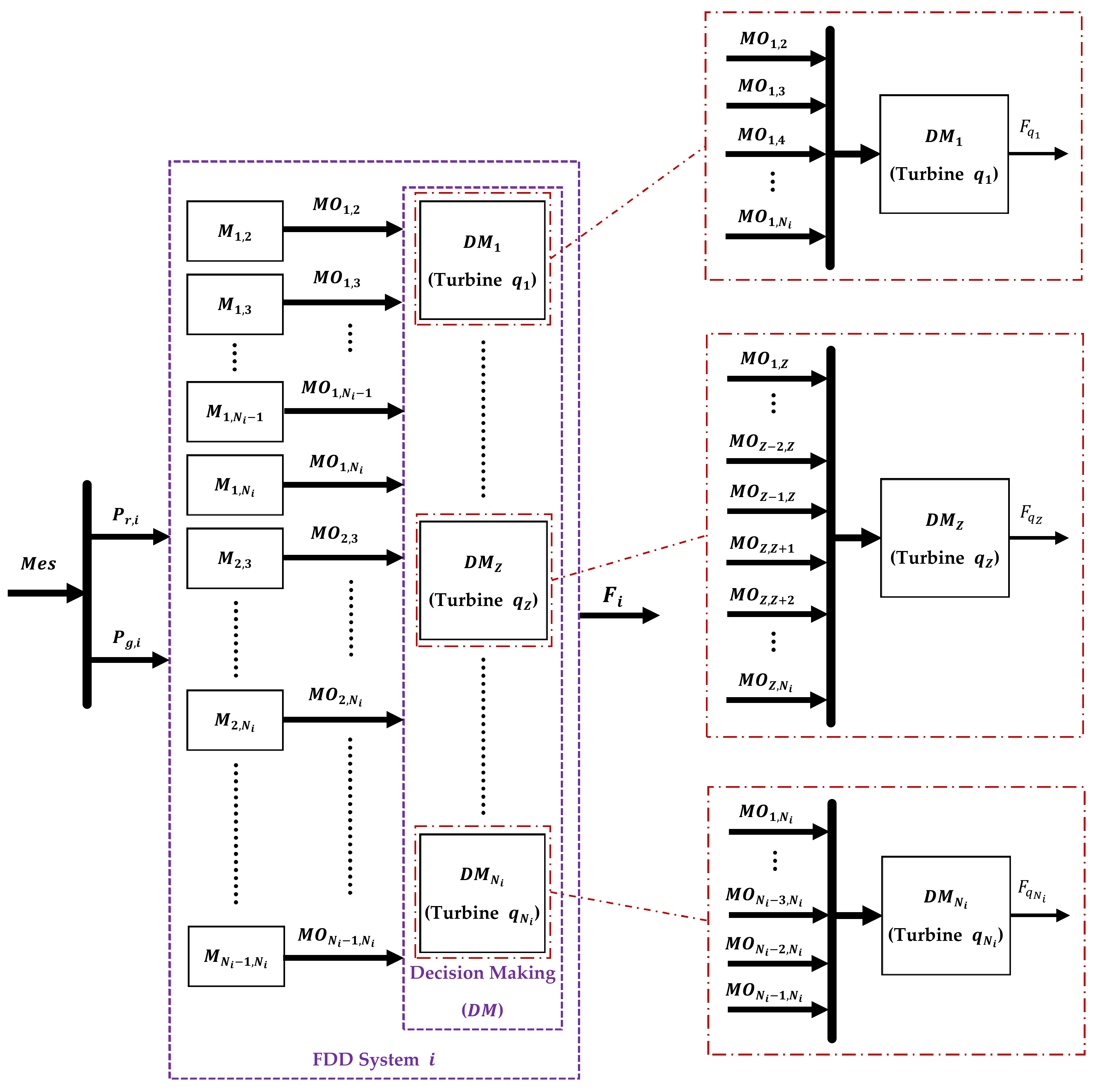
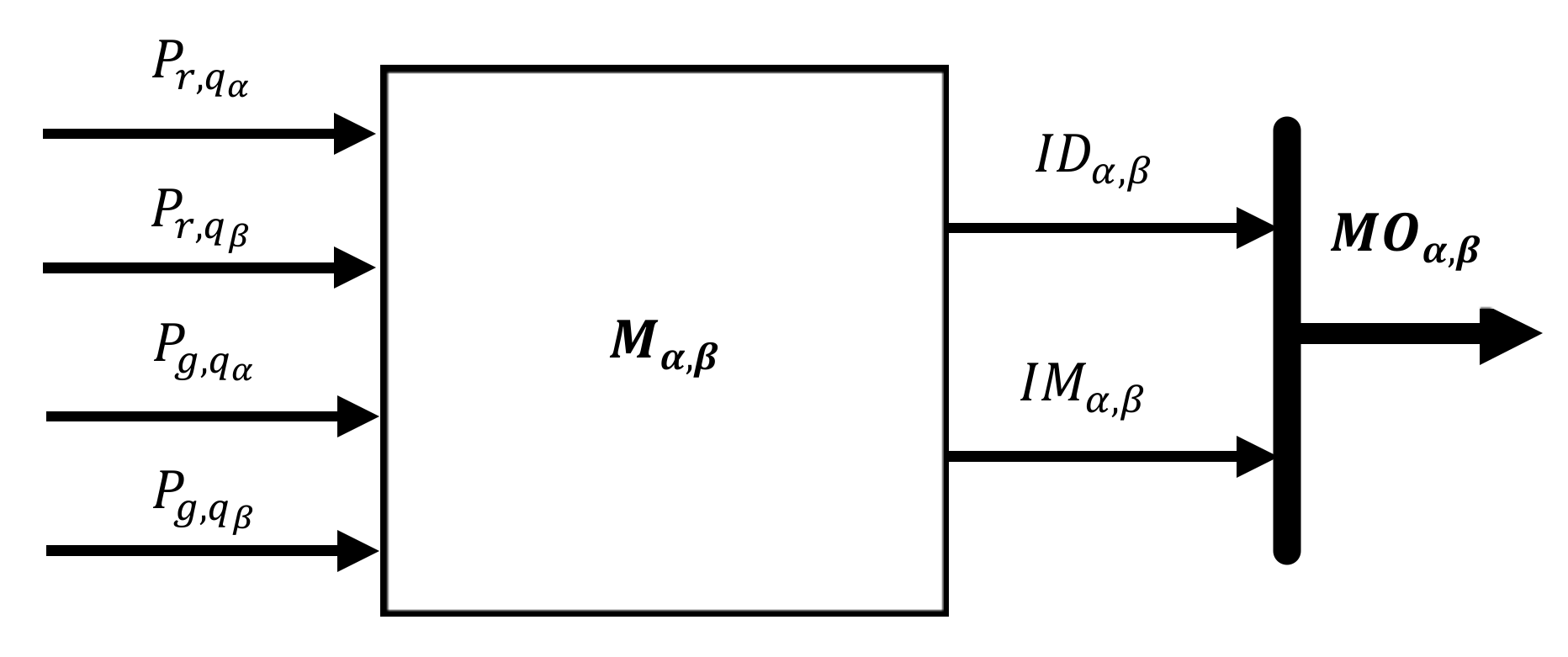
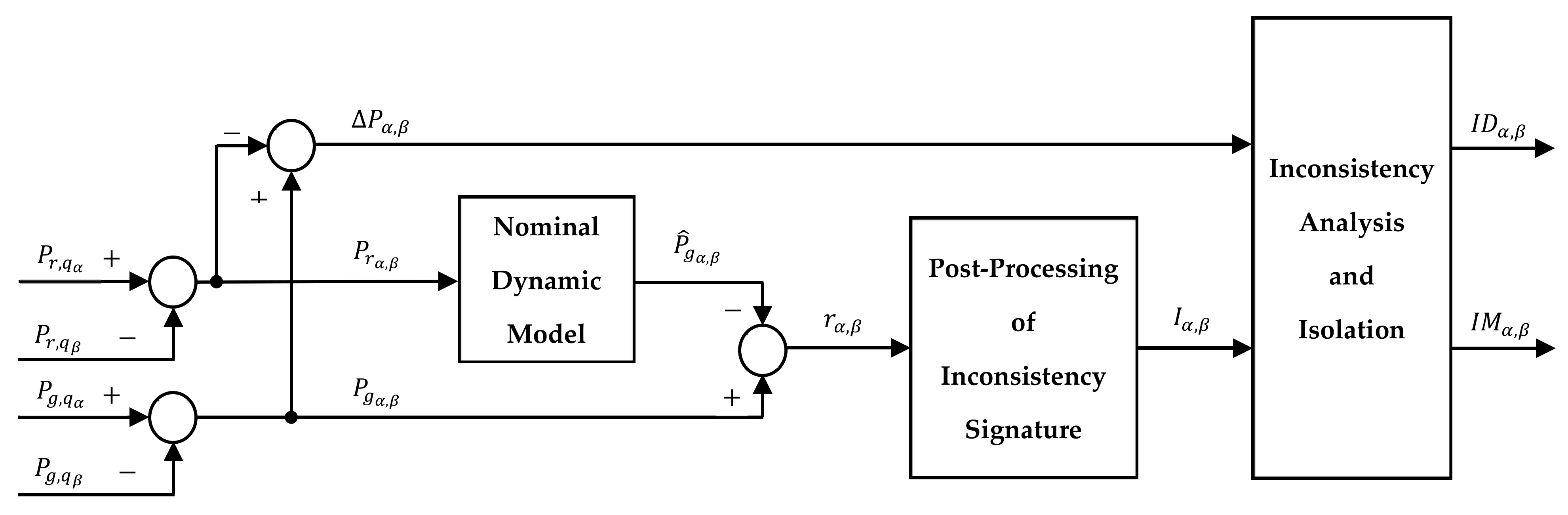
3.1. Distributed FDD Systems

Before providing more information about the design of the distributed FDD system, it should be pointed out that handling the considered power loss faults at the turbine level is a difficult task. To further explain, a lower generated power can occur because of debris build-up on the turbine’s blades, or simply that the real wind speed is less than the measured/estimated wind speed. It should be pointed out that at the farm level, it is possible to monitor and compare the performance and other dynamic features of different turbines in the farm (as a part of the cluster) [20]. In the present paper, the FDD approach introduced in [20] is extended to a larger level at the WFC level. More precisely, the proposed FDD approach in [20] is applied on each wind farm in the WFC. As discussed in this section, the wind farm clustering approach results in a more efficient programming and substantially lower computational cost, all of which are important when implementing an active FTCC scheme in large-scale wind farms or WFCs.

Without loss of generality, the distributed FDD system in Figure 3 and Figure 4 is used to provide real-time information about the true status of each turbine in the cluster. More precisely, the FDD systems deal with the considered power-loss faults at the WFC level by monitoring the consistency of produced power from all turbines in each farm in real time. Therefore, any inconsistencies in produced power are detected and identified to obtain reliable FDD information. Such a fault-monitoring and FDD scheme can be achieved by the model-based algorithm presented in [20]. As a matter of fact, real-time consistency monitoring of the powers from different wind turbines (in a farm or cluster) is not a straightforward procedure even in the case of adjacent wind turbines where wind properties might be almost similar. In fact, for different turbines in a farm, the power reference signals are not necessarily the same, and thus the turbines’ generated power might be different even during fault-free or normal conditions. Given that, in order to correctly monitor the power consistency generated from any two arbitrary turbines, it is important to consider not only their generated power, but also their power reference signals.

An effective approach is to monitor the consistency of produced power online from any individual turbine and all other turbines in the farm. To further explain, consider wind farm $Q_i$ with $N_i$ turbines that are labeled as$q_1,q_2,\dots ,q_{N_i}$. Thus, the simultaneous consistency monitoring of generated powers needs $R_i$ similar modules as shown in Equation (6).

$$R_i=1+2+3+\cdots +\left(N_i-1\right)=\frac{N_i\left(N_i-1\right)}{2}$$

(6)

Table 2. Required $R_i$ modules for a farm with $N_i$ wind turbines.

	${\mathit{q}}_{\mathbf{1}}$	${\mathit{q}}_{\mathbf{2}}$	${\mathit{q}}_{\mathbf{3}}$	${\mathit{q}}_{\mathbf{4}}$	${\mathit{q}}_{\mathbf{5}}$	${\mathit{q}}_{\mathbf{6}}$	${\mathit{q}}_{\mathbf{7}}$	${\mathit{q}}_{\mathbf{8}}$	${\mathit{q}}_{\mathbf{9}}$	${\mathit{q}}_{\mathbf{10}}$	$\cdots$	${\mathit{q}}_{{\mathit{N}}_{\mathit{i}}\mathbf{-}\mathbf{1}}$	${\mathit{q}}_{{\mathit{N}}_{\mathit{i}}}$
${\mathit{q}}_{\mathbf{1}}$		$M_{1,2}$	$M_{1,3}$	$M_{1,4}$	$M_{1,5}$	$M_{1,6}$	$M_{1,7}$	$M_{1,8}$	$M_{1,9}$	$M_{1,10}$	$\cdots$	$M_{1,N_i-1}$	$M_{1,N_i}$
${\mathit{q}}_{\mathbf{2}}$			$M_{2,3}$	$M_{2,4}$	$M_{2,5}$	$M_{2,6}$	$M_{2,7}$	$M_{2,8}$	$M_{2,9}$	$M_{2,10}$	$\cdots$	$M_{2,N_i-1}$	$M_{2,N_i}$
${\mathit{q}}_{\mathbf{3}}$				$M_{3,4}$	$M_{3,5}$	$M_{3,6}$	$M_{3,7}$	$M_{3,8}$	$M_{3,9}$	$M_{3,10}$	$\cdots$	$M_{3,N_i-1}$	$M_{3,N_i}$
${\mathit{q}}_{\mathbf{4}}$					$M_{4,5}$	$M_{4,6}$	$M_{4,7}$	$M_{4,8}$	$M_{4,9}$	$M_{4,10}$	$\cdots$	$M_{4,N_i-1}$	$M_{4,N_i}$
${\mathit{q}}_{\mathbf{5}}$						$M_{5,6}$	$M_{5,7}$	$M_{5,8}$	$\cdots$	$M_{5,10}$	$\cdots$	$M_{5,N_i-1}$	$M_{5,N_i}$
${\mathit{q}}_{\mathbf{6}}$							$M_{6,7}$	$M_{6,8}$	$M_{6,9}$	$M_{6,10}$	$\cdots$	$M_{6,N_i-1}$	$M_{6,N_i}$
${\mathit{q}}_{\mathbf{7}}$								$M_{7,8}$	$M_{7,9}$	$M_{7,10}$	$\cdots$	$M_{7,N_i-1}$	$M_{7,N_i}$
${\mathit{q}}_{\mathbf{8}}$									$M_{8,9}$	$M_{8,10}$	$\cdots$	$M_{8,N_i-1}$	$M_{8,Ni}$
${\mathit{q}}_{\mathbf{9}}$										$M_{9,10}$	$\cdots$	$M_{9,N_i-1}$	$M_{9,N_i}$
${\mathit{q}}_{\mathbf{10}}$											$\cdots$	$M_{10,N_i-1}$	$M_{10,N_i}$
$\mathbf{⋮}$												$⋮$	$⋮$
${\mathit{q}}_{{\mathit{N}}_{\mathit{i}}\mathbf{-}\mathbf{1}}$													$M_{N_i-1,N_i}$

shows the formation of required modules (each denoted by an$M$) for the farm $Q_i$ with $N_i$ wind turbines. Each module from this table monitors the consistency of the generated power from two different wind turbines in the farm. For instance, $M_{\alpha ,\beta }$ with $\alpha \ne \beta$ represents the module that monitors the consistency of the produced power from turbine $q_{\alpha }$ and turbine $q_{\beta }$ in a wind farm. Considering a farm with ten wind turbines ($N_i$ = 10), 45 modules ($R_i$ = 45) are needed to monitor the entire wind farm. However, for a large-scale wind farm or WFC, for example, with 100 wind turbines, the FDD scheme in [20] requires 4950 modules ($R_i=\frac{100\left(100-1\right)}{2}=4950$) that would be computationally expensive to implement. To address such a problem, this study suggests a novel clustering approach which significantly reduces the number of modules involved in the FDD computations. Applying the clustering approach in this paper, a large-scale wind farm or WFC is divided into a group of smaller scale wind farms for which a significantly lower number of modules would be required. For instance, in case of the WFC with 100 wind turbines, this can be divided into a group of small-scale wind farms (e.g., 10 wind farms with equal number of 10 wind turbines in each wind farm) for which the required number of modules is significantly reduced from 4950 to 450 modules. That is, each of the 10 wind farms has an FDD system with 45 modules ($R_i=\frac{10\left(10-1\right)}{2}=45$) which makes a total of 450 modules, i.e., more than 10 times less than the required 4950 modules in [20].

An FDD system’s general structure is illustrated in Figure 5. As seen, it includes $R_i$ modules (already listed in Table 2) and a group of decision making ($DM$) blocks ($D{M}_1,D{M}_2,\dots ,D{M}_{N_i}$) that each relates to an individual wind turbine. Each $DM$ block analyses the relevant module output ($MO$) signals to make decision about the status of its corresponding wind turbine in real-time. In Figure 5, $Mes$ denotes a performance vector including measured variables as well as control commands (or references) in the wind turbines. The FDD system in each wind farm only requires the sets of reference and generated power values that are defined in Equations (7) and (8), respectively.

$$P_{r,i}\left(k\right)=\left[P_{r,q_j}\left(k\right)\right] , q_j\in Q_i$$

(7)

$$P_{g,i}\left(k\right)=\left[P_{g,q_j}\left(k\right)\right] , q_j\in Q_i$$

(8)

Here, the reference powers denoted by $P_{r,q_j}$ are computed according to [20] as:

$$P_{r,q_j}\left(k\right)={\tau }_{r,q_j}\left(k\right){\omega }_{g,q_j}\left(k\right)$$

(9)

where ${\tau }_{r,q_j}$ and ${\omega }_{g,q_j}$ denote the reference generator torque and the angular speed of generator for wind turbine $q_j$ in the farm $Q_i$, respectively. Each module in Figure 5 has its respective inputs and outputs. For instance, Figure 6 illustrates module $M_{\alpha ,\beta }$ with its appropriate inputs and outputs. This module with $\alpha \ne \beta$ monitors the consistency of generated powers from turbine $q_{\alpha }$ and turbine $q_{\beta }$ in the farm $Q_i$. In Figure 6, the module’s inputs include the reference powers ($P_{r,q_{\alpha }}, P_{r,q_{\beta }}$) and the generated powers ($P_{g,q_{\alpha }}, P_{g,q_{\beta }}$) in the relevant wind turbines $q_{\alpha }$ and $q_{\beta }$, whereas the module’s output vector $M{O}_{\alpha ,\beta }$includes inconsistency detection ($I{D}_{\alpha ,\beta }$) and inconsistency magnitude ($I{M}_{\alpha ,\beta }$) signals. $I{D}_{\alpha ,\beta }$ and $I{M}_{\alpha ,\beta }$ signals indicate, respectively, the occurrence and the magnitude of any possible inconsistencies in the produced powers from turbines $q_{\alpha }$ and$q_{\beta }$. Under two possible cases for the power consistency by turbines $q_{\alpha }$ and$q_{\beta }$, the module’s output vector $M{O}_{\alpha ,\beta }$may attain the values indicated in

Table 3. Possible cases for module output vector $M{O}_{\alpha ,\beta }$ considering example module $M_{\alpha ,\beta }$.

${\mathit{q}}_{\mathit{\alpha }}$ and ${\mathit{q}}_{\mathit{\beta }}$ Power Consistency	Module Output $\mathit{M}{\mathit{O}}_{\mathit{\alpha }\mathbf{,}\mathit{\beta }}$
	$\mathit{I}{\mathit{D}}_{\mathit{\alpha }\mathbf{,}\mathit{\beta }}$	$\mathit{I}{\mathit{M}}_{\mathit{\alpha }\mathbf{,}\mathit{\beta }}$
Consistent	$0$	$0$
Inconsistent	$\alpha$	$\left|{\overline{\Delta P}}_{\alpha ,\beta }\right|$
	$\beta$	$\left|{\overline{\Delta P}}_{\alpha ,\beta }\right|$

. As observed in the table, if power production is inconsistent between turbines $q_{\alpha }$ and $q_{\beta }$, the $I{D}_{\alpha ,\beta }$, $I{M}_{\alpha ,\beta }$ signals indicate the faulty turbine along with its absolute value of the estimated power-loss$\left|{\overline{\Delta P}}_{\alpha ,\beta }\right|$, respectively. Conversely, if power production is consistent between turbines $q_{\alpha }$ and $q_{\beta }$, both $I{D}_{\alpha ,\beta }$ and $I{M}_{\alpha ,\beta }$ signals become zero. Note that obtaining such zero signals (in the latter case) does not necessarily mean that both turbines $q_{\alpha }$ and $q_{\beta }$ are healthy. As a matter of fact, if power production is consistent between two considered turbines they may either be both healthy or faulty. Given that, as can be seen in Figure 5, the FDD system employs a set of $DM$ blocks to analyse the modules outputs all together in real-time and identify any faulty turbine(s) accordingly.

As mentioned, Figure 5 shows the appropriate distribution and contribution of module outputs in the decision-making procedure within each $DM$ block. Each individual wind turbine has a $DM$ block that is exclusively used to analyse the $MO$ signals related to that individual wind turbine and, accordingly, make an appropriate decision about the wind turbine’s real-time health status. The simple logic behind such a decision is that as long as at least one of the relevant modules detects a turbine as a faulty turbine, then that turbine is faulty and its power-loss due to the fault (i.e., ${\widehat{\mathcal{P}}}_{q_j}$) is conservatively the maximum power-loss estimated by the modules [20]. As per the given information in Figure 5 and Figure 6 and Table 3, the aforementioned decision-making logic can be formulated as in $Rule 1$, $Rule Z$ and $Rule N_i$ for turbines $q_1$, $q_Z$ and$q_{N_i}$, respectively [20]. Note that $q_Z$ with ($Z\in \mathbb{N}$ and $1<Z<N_i$) denotes any wind turbine except $q_1$ or $q_{N_i}$.

Rule 1:

$$\begin{array}{c}If \left(I{D}_{1,2}=1\right) OR \left(I{D}_{1,3}=1\right) OR \left(I{D}_{1,4}=1\right) OR\dots OR \left(I{D}_{1,N_i}=1\right),\\ Then q_1 is faulty and {\widehat{\mathcal{P}}}_{q_1}=max\left\{I{M}_{1,2},I{M}_{1,3},I{M}_{1,4},\dots ,I{M}_{1,N_i}\right\}\end{array}$$

Rule Z:

$$\begin{array}{c}If \left(I{D}_{1,Z}=Z\right) OR\dots OR \left(I{D}_{Z-2,Z}=Z\right) OR \left(I{D}_{Z-1,Z}=Z\right) OR \left(I{D}_{Z,Z+1}=Z\right) OR \left(I{D}_{Z,Z+2}=Z\right) OR\dots OR \left(I{D}_{Z,N_i}=Z\right),\\ Then q_Z is faulty and {\widehat{\mathcal{P}}}_{q_Z}=max\left\{I{M}_{1,Z},\dots ,I{M}_{Z-2,Z},I{M}_{Z-1,Z},I{M}_{Z,Z+1},I{M}_{Z,Z+2}\dots ,I{M}_{Z,N_i}\right\}\end{array}$$

Rule N_i:

$$\begin{array}{c}If \left(I{D}_{1,N_i}=N_i\right) OR\dots OR \left(I{D}_{N_i-3,N_i}=N_i\right) OR \left(I{D}_{N_i-2,N_i}=N_i\right) OR \left(I{D}_{N_i-1,N_i}=N_i\right),\\ Then q_{N_i} is faulty and {\widehat{\mathcal{P}}}_{q_{N_i}}=max\left\{I{M}_{1,N_i},\dots ,I{M}_{N_i-3,N_i},I{M}_{N_i-2,N_i},I{M}_{N_i-1,N_i}\right\}\end{array}$$

Outcomes obtained from $DM$ blocks (see Figure 5) include the FDD information vector $F_i$ in Equation (10) for the wind farm $Q_i$ in the cluster.

$$F_i\left(k\right)=\left[F_{q_j}\left(k\right)\right] , q_j\in Q_i$$

(10)

where $F_{q_j}\left(k\right)$ includes the number of wind turbine $q_j$ and its power-loss magnitude ${\widehat{\mathcal{P}}}_{q_j}$. Apparently, the functionality of the FDD system described here depends on the monitoring process in the modules. From a design perspective, the entire modules utilized in the distributed FDD system are the same, although each one corresponds a particular pair of wind turbines. Every module uses a dynamic model of the nominal system, which is developed by a data-driven modelling technique based on fuzzy modeling and identification (FMI) approach [31]. Indeed, the dynamic model estimates the nominal relative performance between wind turbines $q_{\alpha }$ and $q_{\beta }$ in wind farm $Q_i$. The following paragraphs provide more information about the internal structure of the modules.

Module Structure: Figure 7 illustrates the internal structure of module $M_{\alpha ,\beta }$. As can be seen, the module uses a dynamic model that is represented by a Takagi-Sugeno (T-S) type fuzzy model. More details about T-S type fuzzy modeling approach are available in the literature [20,31]. The mentioned model estimates the nominal relative behavior between turbines $q_{\alpha }$ and $q_{\beta }$ in wind farm $Q_i$. The generated powers from turbines $q_{\alpha }$ and $q_{\beta }$ are defined as consistent when $P_{g_{\alpha ,\beta }}$ and ${\widehat{P}}_{g_{\alpha ,\beta }}$ are approximately equal (or the residual signal $r_{\alpha ,\beta }$ is almost zero). In practice, this equality can not happen at all times, mainly due to measurement noises, possible disturbances and model uncertainties. For this reason, a post-processing of inconsistency signature unit is used to achieve absolute inconsistency $I_{\alpha ,\beta }$. It should be noted that $I_{\alpha ,\beta }$ has binary values (i.e., 0 for consistent power generation and 1 for inconsistent power generation). The post-processing unit utilizes a threshold test technique to obtain a reliable conclusion for $I_{\alpha ,\beta }$. In more detail, in the case of any inconsistency occurrence in the power generation, $I_{\alpha ,\beta }$ switches from 0 to 1 if $r_{\alpha ,\beta }$ remains outside a predefined threshold $T_{\alpha ,\beta }$ for more than $t_{in}$ consecutive time-steps. Then, $I_{\alpha ,\beta }$ switches from 1 to 0 if $r_{\alpha ,\beta }$ remains within $T_{\alpha ,\beta }$ for more than $t_{out}$ consecutive time-steps. The appropriate values for $T_{\alpha ,\beta }$, $t_{in}$, and $t_{out}$ can be determined by the designer. It should be noted that $I_{\alpha ,\beta }$ only indicates the consistency or inconsistency between considered turbines. In other words, $I_{\alpha ,\beta }$ does not include any information about the magnitude of the power-loss fault. Therefore, the inconsistency analysis and isolation unit is used to isolate the faulty turbine and identify the magnitude of fault. During any inconsistency (i.e., $I_{\alpha ,\beta }=1$), this unit computes the running mean of $\Delta P_{\alpha ,\beta }$ as ${\overline{\Delta P}}_{\alpha ,\beta }$. Note that if (${\overline{\Delta P}}_{\alpha ,\beta }<0$) then $q_{\alpha }$ is faulty, and if (${\overline{\Delta P}}_{\alpha ,\beta }>0$) then $q_{\beta }$ is faulty.

3.2. Integrated ASC Unit

At the turbine level, and in the event of possible mild power loss faults, the proposed active FTCC scheme enables fault-tolerant capability for generator torque controller in any faulty wind turbine(s) inside each farm. More precisely, this control solution accommodates fault effects in faulty wind turbine(s) whose loss of generated power is/are mild (normally less than 3%). Such mildly faulty turbines are still healthy enough to continue their operations although an appropriate signal correction is required in their generator torque controllers. As previously discussed in Section 2.2, the mentioned power loss fault results in a lower power production that adversely affects the total active power produced by all the turbines in WFC as a whole. When a mild power loss fault occurs in one or more than one turbine in a cluster’s wind farms, the relevant wind farm controller should follow the network operator’s demanded power $P_{D,Q_i}$ in Equation (4), no matter which turbine or turbines are mildly faulty. However, the compensation of power loss in mildly faulty wind turbine(s) is preferred to prevent overloading the remaining healthy wind turbines. Instead, the power reference signal(s) to the faulty wind turbine(s) is/are corrected in order to accommodate the mild fault effects. As shown in Figure 3, ASC units are responsible for the described accommodation of mild power loss faults at the turbine level inside the cluster’s individual wind farms and according to their respective FDD information. Indeed, providing the most up-to-date information about the status of WFC, the distributed FDD systems enable ASC units to automatically safeguard the entire WFC. To explain further, any inconsistencies in the generated powers are identified to generate reliable FDD information. Finally, this online information is utilized for ASC and accommodation of the mild power loss faults in faulty wind turbines. The ASC mechanism does not interfere with the normal operation of baseline controllers at the turbine or farm levels, but only corrects the output of torque control system in faulty wind turbine(s) based on the online fault information received from the FDD system. The ASC units in Figure 3 are not described explicitly here since they are very simple algorithms. According to the provided FDD information in each wind farm, the relevant ASC unit identifies the faulty wind turbines along with their relevant fault magnitudes (estimated mild power losses). Accordingly, the estimated fault magnitudes are used to correct the generator reference torque signals ${\tau }_{r,q_j}$ computed by the torque control system. This simple signal correction mechanism is shown in Equation (11) for the $q_j$th turbine in the farm $Q_i$.

$${\tau }_{r,q_j,corr}\left(k+1\right)={\tau }_{r,q_j}\left(k\right)+\frac{{\widehat{\mathcal{P}}}_{q_j}\left(k\right)}{{\omega }_{g,q_j}\left(k\right)} , q_j\in Q_i$$

(11)

In Equation (11), ${\tau }_{r,q_j}$ and ${\omega }_{g,q_j}$ denote the generator reference torque and generator angular speed for the $q_j$th turbine in the farm $Q_i$, respectively. The corrected reference generator torque is denoted by ${\tau }_{r,q_j,corr}$, whereas ${\widehat{\mathcal{P}}}_{q_j}$ is the estimated fault magnitude, both in the $q_j$th turbine in the farm $Q_i$. Under fault-free conditions, ${\widehat{\mathcal{P}}}_{q_j}$ is assigned to be zero to keep the system’s nominal performance. To avoid excessive loadings on the actuators, the recommended rate and magnitude limiters are used for ${\tau }_{r,q_j,corr}$ computed by Equation (11).

3.3. Fault-Tolerant Wind Farm Controller

In the event of severe power loss faults (normally more than 3%) in wind turbines, the ASC mechanism at the turbine level is not sufficient. Thus, a hierarchical control reallocation mechanism in two higher levels is required. The first control reallocation level, referred to as “farm-level control reallocation”, relies on the turbines’ health factors obtained by Algorithm 1. In order to compensate the missing power of severely faulty wind turbines, this farm-level control reallocation mechanism automatically reallocates control commands among turbines in each wind farm to demand healthier wind turbines to produce more power. If healthier wind turbines in a respective farm do not have enough available power to accommodate severe fault effects, a higher control reallocation level, referred to as “WFC-level control reallocation” (inside the fault-tolerant network operator in Figure 3 and Figure 4) is activated automatically. This top layer of control is discussed in the next subsection.

In line with the proposed solution in [22], the online health status of turbine $q_j$ in farm $Q_i$ is represented using the binary health factor $H{f}_{q_j}=\left\{0, 1\right\}$. That is, for healthy or mildly faulty wind turbines, the health factor attains 1, whereas for severely faulty turbines this factor attains 0. The farm-level control reallocation mechanism uses these health factors to appropriately switch between nominal control and control reallocation modes. In more detail, when all health factors of wind turbines are 1, the farm controller operates under nominal control mode as per Equation (4). However, the signal correction by ASC units (at wind turbine level) might be needed to accommodate mild power loss faults as discussed in previous subsection. In the event of any severe fault in any turbine of farm $Q_i$, the turbine’s respective health factor changes to 0. Accordingly, the farm controller switches to the reallocation mode. As such, the wind farm’s healthier wind turbines with extra (unused) available power take over the pending duties of the severely faulty wind turbines. This strategy ensures safe and continuous operation of farm $Q_i$ following the farm’s demanded power.

According to [22], under the farm-level control reallocation mode, a wind farm controller initially computes the missed power in severely faulty wind turbines (with $Hf=0$) as follows:

$$P_{m,q_j}\left(k\right)=P_{d,q_j}\left(k\right)-P_{g,q_j}\left(k\right)$$

(12)

$$P_{M,Q_i}\left(k\right)={\displaystyle \sum }_{q_j\in \{Q_i | H{f}_{q_j}=0\}}{P}_{m,q_j}\left(k\right)$$

(13)

in which $P_{d,q_j}\left(k\right)$, $P_{g,q_j}\left(k\right)$, and $P_{m,q_j}\left(k\right)$ are, respectively, the demanded, generated, and missed powers in turbine$q_j$ from farm $Q_i$ at the time-instant (time-step) $k$. Moreover, $P_{M,Q_i}\left(k\right)$ in Equation (13) is the total missed power in severely faulty turbines at the time-step$k$. This amount of total missed power must be compensated for by demanding the healthier turbines (with $Hf=1$) to produce more power if they have extra available power computed by:

$$P_{u,q_j}\left(k\right)=P_{a,q_j}\left(k\right)-P_{g,q_j}\left(k\right)$$

(14)

$$P_{U,Q_i}\left(k\right)={\displaystyle \sum }_{q_j\in \{Q_i| H{f}_{q_j}=1\}}{P}_{u,q_j}\left(k\right)$$

(15)

in which $P_{a,q_j}\left(k\right)$ and $P_{u,q_j}\left(k\right)$ respectively denote the estimated available power and the extra available power in turbine $q_j$ from farm $Q_i$ at the time-step $k$. Note that, $P_{U,Q_i}\left(k\right)$ in Equation (15) represents the total extra available power in healthier turbines in the same farm. A wind turbine’s available power is estimated according to Equation (5), and the estimated total available power in farm $Q_i$ is given by:

$$P_{A,Q_i}\left(k\right)={\displaystyle \sum }_{j=1}^{N_i}{P}_{a,q_j}\left(k\right) , Q_i\in Q$$

(16)

Lastly, the demanded power from healthier turbines (with $Hf=1$) is obtained as:

$$\begin{gathered} P_{d,q_j}\left(k+1\right)=P_{D,Q_i}\left(k+1\right)\frac{P_{a,q_j}\left(k\right)}{P_{A,Q_i}\left(k\right)}+P_{M,Q_i}\left(k\right)\frac{P_{u,q_j}\left(k\right)}{P_{U,Q_i}\left(k\right)} , \\ {q}_j\in \{Q_i|H{f}_{q_j}=1\} \end{gathered}$$

(17)

where $P_{d,q_j}\left(k+1\right)$ and $P_{D,Q_i}\left(k\right)$ are the already defined variables for Equation (4). Algorithm 1 presents the entire details of the described farm-level control reallocation mechanism.

Algorithm 1. Wind Farm $Q_i$ Control Reallocation (Active FTCC at Secondary Control Level).
	Inputs:$\left\{P_{D,Q_i}\left(k+1\right),P_{g,q_j}\left(k\right),V_{mes,q_j}\left(k\right),F_{q_j}\left(k\right)|i,j\in \mathbb{N}, i\le N,j\le N_i\right\}$ $\mathbb{N}$: natural numbers set $N$: number of wind farms in a wind farm cluster, $N_i$: number of wind turbines in wind farm $Q_i$, $k$: time-step, $P_{D,Q_i}\left(k+1\right)$: total demanded power from wind farm $Q_i$ for the next time-step, $P_{g,q_j}\left(k\right)$: generated (output) power of wind turbine $q_j$, $V_{mes,q_j}\left(k\right)$: measured nacelle wind speed of wind turbine $q_j$, and $F_{q_j}\left(k\right)$: fault information including the number of wind turbine $q_j$ and its power loss magnitude ${\widehat{\mathcal{P}}}_{q_j}$. Outputs: $\left\{\left\{P_{d,q_j}\left(k+1\right)|q_j\in Q_i\right\},P_{A,Q_i}\left(k\right),P_{G,Q_i}\left(k\right),H{F}_{Q_i}\left(k\right)\right\}$ $Q_i=\left\{q_j| j\in \mathbb{N},j\le N_i\right\}$: set of wind turbines in wind farm $Q_i$, $P_{d,q_j}\left(k+1\right)$: demanded power from wind turbine $q_j$ for the next time-step, $P_{A,Q_i}\left(k\right)$: total available power in wind farm $Q_i$,$P_{G,Q_i}\left(k\right)$: total generated power in wind farm $Q_i$, and $H{F}_{Q_i}\left(k\right)$: total health factor of wind farm $Q_i$. Constants and Variables: $\left\{P_{rated,q_j},\rho ,R,C_{Pmax},T_{Q_i},T_{q_j},P_{d,q_j}\left(k\right),P_{a,q_j}\left(k\right),P_{m,q_j}\left(k\right),P_{u,q_j}\left(k\right),P_{M,Q_i}\left(k\right),P_{U,Q_i}\left(k\right),H{f}_{q_j}\left(k\right)\right\}$ $P_{rated,q_j}$: rated power of wind turbine $q_j$, $\rho$: air density, $R$: rotor radius, $C_{Pmax}$: maximum power coefficient,$T_{Q_i}$: threshold for severe fault detection in wind farm $Q_i$, $T_{q_j}$: threshold for severe fault detection in wind turbine $q_j$,$P_{d,q_j}\left(k\right)$: demanded power for turbine $q_j$, $P_{a,q_j}\left(k\right)$: available power in turbine $q_j$, $P_{m,q_j}\left(k\right)$: missed power of turbine $q_j$, $P_{u,q_j}\left(k\right)$: extra available power in turbine $q_j$, $P_{M,Q_i}\left(k\right)$: total missed power of wind farm $Q_i$, and $P_{U,Q_i}\left(k\right)$: total extra available power of farm $Q_i$, and $H{f}_{q_j}\left(k\right)=\left\{0,1\right\}$: health factor for turbine $q_j$.
1. for each $q_j\in Q_i$ do     1.1. if ${\widehat{\mathcal{P}}}_{q_j}\ge T_{q_j}$ then          1.1.1. $H{f}_{q_j}\left(k\right)=0$     1.2. else if ${\widehat{\mathcal{P}}}_{q_j}<T_{Q_i}$ then          1.2.1. $H{f}_{q_j}\left(k\right)=1$     1.3. end if     1.4. $P_{a,q_j}\left(k\right)=minimum\left\{P_{rated,q_j},\frac{\pi }{2}\rho R^2{V}_{mes,q_j}{\left(k\right)}^3{C}_{Pmax}\right\}$     1.5.  $P_{m,q_j}\left(k\right)=P_{d,q_j}\left(k\right)-P_{g,q_j}\left(k\right)$     1.6.  $P_{u,q_j}\left(k\right)=P_{a,q_j}\left(k\right)-P_{g,q_j}\left(k\right)$   2. end for   3. $P_{A,Q_i}\left(k\right)={\displaystyle \sum }_{j=1}^{N_i}{P}_{a,q_j}\left(k\right)$   4.  $P_{G,Q_i}\left(k\right)={\displaystyle \sum }_{j=1}^{N_i}{P}_{g,q_j}\left(k\right)$   5.  $P_{M,Q_i}\left(k\right)={\displaystyle \sum }_{q_j\in \left\{Q_i\right|H{f}_{q_j}=0\}}{P}_{m,q_j}\left(k\right)$   6.  $P_{U,Q_i}\left(k\right)={\displaystyle \sum }_{q_j\in \left\{Q_i\right|H{f}_{q_j}=1\}}{P}_{u,q_j}\left(k\right)$   7. for each $q_j\in \{Q_i|H{f}_{q_j}=0\}$ do     7.1. $P_{d,q_j}\left(k+1\right)=P_{D,Q_i}\left(k+1\right)\frac{P_{a,q_j}\left(k\right)}{P_{A,Q_i}\left(k\right)}$   8. end for   9. for each $q_j\in \{Q_i|H{f}_{q_j}=1\}$ do     9.1. $P_{d,q_j}\left(k+1\right)=P_{D,Q_i}\left(k+1\right)\frac{P_{a,q_j}\left(k\right)}{P_{A,Q_i}\left(k\right)}+P_{M,Q_i}\left(k\right)\frac{P_{u,q_j}\left(k\right)}{P_{U,Q_i}\left(k\right)}$   10. end for   11. if $\frac{1}{N_i}{\displaystyle \sum }_{j=1}^{N_i}H{f}_{q_j}\left(k\right)\ge T_{Q_i}$ then     11.1. $H{F}_{Q_i}\left(k\right)=1$   12. else if $\frac{1}{N_i}{\displaystyle \sum }_{j=1}^{N_i}H{f}_{q_j}\left(k\right)<T_{Q_i}$ then     12.1. $H{F}_{Q_i}\left(k\right)=0$   13. end if   14. return $P_{A,Q_i}\left(k\right)$, $P_{G,Q_i}\left(k\right)$, $H{F}_{Q_i}\left(k\right)$, and $\left\{P_{d,q_j}\left(k+1\right)|q_j\in Q_i\right\}$

3.4. Fault-Tolerant Network Operator

According to Algorithm 1, the health status of farm $Q_i$ (inside the WFC $Q$) is represented by its respective binary health factor $H{F}_{Q_i}\left(k\right)=\left\{0, 1\right\}$ that is determined by a threshold-based detection method. In fact, for fault-free wind farms or faulty wind farms with mild power loss fault, the health factor is 1, whereas for faulty wind farms with severe power loss fault, the health factor is 0. In other words, when $H{F}_{Q_i}=1$, the faults effects can be accommodated at the farm level using the ASC unit and fault-tolerant wind farm controller in farm $Q_i$. However, when $H{F}_{Q_i}=0$, the fault accommodation at the farm level is not sufficient due to the lack of enough available power in the farm. In this case, the control commands is automatically reallocated among the farms at the WFC level to require healthier farms (with an extra available power) to produce more power and compensate the missing power of the farms impacted by severe power loss.

Here, the network operator employs the health factors $H{F}_{Q_i}$ from wind farm $Q_i$ to appropriately switch between nominal control and control reallocation modes, but at the WFC level. When all wind farms have health factors of 1, the network operator works under the nominal control mode as in Equation (3). In such a case, only signal correction at the turbine level and control reallocation at the wind farm level might be required to accommodate possible power loss faults as previously described. Conversely, as soon as any severe power loss fault is detected in any wind farm of the WFC, the wind farm’s respective health factor changes to 0. As a result, the network operator switches to the reallocation mode in which healthier wind farms (with extra available power) take over the pending duties of the faulty farm(s). Thus, the safe and uninterrupted operation of the WFC as a whole is guaranteed.

Under the WFC-level control reallocation mode, the network operator first computes the missed power in wind farms impacted by severe fault ($HF=0$) as shown below:

$$P_{M,Q_i}\left(k\right)=P_{D,Q_i}\left(k\right)-P_{G,Q_i}\left(k\right)$$

(18)

$$P_M\left(k\right)={\displaystyle \sum }_{Q_i\in \{Q|H{F}_{Q_i}=0\}}{P}_{M,Q_i}\left(k\right)$$

(19)

where $P_{D,Q_i}\left(k\right)$, $P_{G,Q_i}\left(k\right)$, and $P_{M,Q_i}\left(k\right)$ are, respectively, the demanded, generated, and missed powers for farm $Q_i$ at the time-instant (time-step) $k$. In addition, $P_M\left(k\right)$ in Equation (19) denotes the total missed power in farms with severe power loss at the time-step$k$. This amount of total missed power can be compensated for by requiring the healthier farms (with $HF=1$) to produce more power if they have extra available power. The extra available power in healthier farms is given by

$$P_{U,Q_i}\left(k\right)=P_{A,Q_i}\left(k\right)-P_{G,Q_i}\left(k\right)$$

(20)

$$P_U\left(k\right)={\displaystyle \sum }_{Q_i\in \{Q|H{F}_{Q_i}=1\}}{P}_{U,Q_i}\left(k\right)$$

(21)

where $P_{A,Q_i}\left(k\right)$ and $P_{U,Q_i}\left(k\right)$ are, respectively, the estimated available power and the extra available power in farm $Q_i$ at the time-step$k$. Moreover, $P_U\left(k\right)$ in Equation (21) denotes the total extra available power in healthier farms. Note that the available power in wind farm $Q_i$ is $P_{A,Q_i}\left(k\right)$ (received from the farm controller), and the estimated total available power in the WFC $Q$ is obtained by:

$$P_A\left(k\right)={\displaystyle \sum }_{i=1}^N{P}_{A,Q_i}\left(k\right)$$

(22)

The demanded powers from healthier farms with$HF=1$ are as follows:

$$\begin{gathered} P_{D,Q_i}\left(k+1\right)=P_D\left(k+1\right)\frac{P_{A,Q_i}\left(k\right)}{P_A\left(k\right)}+P_M\left(k\right)\frac{P_{U,Q_i}\left(k\right)}{P_U\left(k\right)} , \\ {Q}_i\in \{Q|H{F}_{Q_i}=1\} \end{gathered}$$

(23)

where $P_{D,Q_i}\left(k+1\right)$ and $P_D\left(k+1\right)$ represent the already defined variables for Equation (3). Algorithm 2 presents the details of the mechanism described for WFC-level control reallocation.

Algorithm 2. Network Operator Control Reallocation (Active FTCC at Tertiary Control Level).
	Inputs:$\left\{P_{A,Q_i}\left(k\right),P_{G,Q_i}\left(k\right),H{F}_{Q_i}\left(k\right),f_{mes}\left(k\right)|i\in \mathbb{N}, i\le N\right\}$ $\mathbb{N}$: natural numbers set, $N$: number of farms in a wind farm cluster, $k$: time-step, $P_{A,Q_i}\left(k\right)$: total available power in wind farm $Q_i$, $P_{G,Q_i}\left(k\right)$: generated (output) power of wind farm $Q_i$, $H{F}_{Q_i}\left(k\right)=\left\{0, 1\right\}$: health factor for wind farm $Q_i$, and $f_{mes}\left(k\right)$: measured grid frequency. Outputs:$\left\{P_{D,Q_i}\left(k+1\right)|Q_i\in Q\right\}$ $Q=\left\{Q_i| i\in \mathbb{N},i\le N\right\}$: set of wind farms in wind farm cluster, $P_{D,Q_i}\left(k+1\right)$: demanded power from wind farm $Q_i$ for the next time-step. Constants and Variables: $\left\{f_r,P_{min},P_{max},c,d,f_e\left(k\right),P_D\left(k+1\right),P_A\left(k\right),P_{D,Q_i}\left(k\right),P_{M,Q_i}\left(k\right),P_{U,Q_i}\left(k\right),P_M\left(k\right),P_U\left(k\right)\right\}$ $f_r$: reference grid frequency, $P_{min}$: minimum limit for total power generated by the wind farm cluster,$P_{max}$: maximum limit for total power generated by wind farm cluster,$c$: control band used for active power control,$d$: dead band used for active power control ($c>d$), $f_e\left(k\right)$: grid frequency error, $P_D\left(k+1\right)$: total demanded power from wind farm cluster for the next time-step, $P_A\left(k\right)$: total available power in wind farm cluster,$P_{D,Q_i}\left(k\right)$: total demanded power from wind farm $Q_i$, $P_{M,Q_i}\left(k\right)$: total missed power of wind farm $Q_i$, $P_{U,Q_i}\left(k\right)$: total extra available power of wind farm $Q_i$,$P_M\left(k\right)$: total missed power in wind farm cluster, and $P_U\left(k\right)$: total extra available power in wind farm cluster.
1. $f_e\left(k\right)=f_{mes}\left(k\right)-f_r$   2. if $f_e\left(k\right)\ge c$ then     2.1. $P_D\left(k+1\right)=P_{min}$   3. else if $d<f_e\left(k\right)<c$ then     3.1. $P_D\left(k+1\right)=\frac{P_{max}+P_{min}}{2}-\frac{\left(P_{max}-P_{min}\right)\left(f_e\left(k\right)-d\right)}{2\left(c-d\right)}$   4. else if $-d\le f_e\left(k\right)\le d$ then     4.1. $P_D\left(k+1\right)=\frac{P_{max}+P_{min}}{2}$   5. else if $-c<f_e\left(k\right)<-d$ then     5.1. $P_D\left(k+1\right)=\frac{P_{max}+P_{min}}{2}-\frac{\left(P_{max}-P_{min}\right)\left(f_e\left(k\right)+d\right)}{2\left(c-d\right)}$   6. else if $f_e\left(k\right)\le -c$ then     6.1. $P_D\left(k+1\right)=P_{max}$   7. end if   8. if $\frac{1}{N}{\displaystyle \sum }_{i=1}^{N}H{f}_{Q_i}\left(k\right)=1$ then     8.1. $P_A\left(k\right)={\displaystyle \sum }_{i=1}^N{P}_{A,Q_i}\left(k\right)$     8.2. for each $Q_i\in Q$ do          8.2.1. $P_{D,Q_i}\left(k+1\right)=P_D\left(k+1\right)\frac{P_{A,Q_i}\left(k\right)}{P_A\left(k\right)}$     8.3. end for   9. else if $\frac{1}{N}{\displaystyle \sum }_{i=1}^{N}H{f}_{Q_i}\left(k\right)<1$ then     9.1. for each $Q_i\in Q$ do          9.1.1. $P_{M,Q_i}\left(k\right)=P_{D,Q_i}\left(k\right)-P_{G,Q_i}\left(k\right)$          9.1.2. $P_{U,Q_i}\left(k\right)=P_{A,Q_i}\left(k\right)-P_{G,Q_i}\left(k\right)$     9.2. end for     9.3. $P_A\left(k\right)={\displaystyle \sum }_{i=1}^N{P}_{A,Q_i}\left(k\right)$     9.4. $P_M\left(k\right)={\displaystyle \sum }_{Q_i\in \{Q|H{F}_{Q_i}=0\}}{P}_{M,Q_i}\left(k\right)$     9.5. $P_U\left(k\right)={\displaystyle \sum }_{Q_i\in \{Q|H{F}_{Q_i}=1\}}{P}_{U,Q_i}\left(k\right)$     9.6. for each $Q_i\in \{Q|H{F}_{Q_i}=0\}$ do          9.6.1. $P_{D,Q_i}\left(k+1\right)=P_D\left(k+1\right)\frac{P_{A,Q_i}\left(k\right)}{P_A\left(k\right)}$     9.7. end for     9.8. for each $Q_i\in \{Q|H{F}_{Q_i}=1\}$ do          9.8.1. $P_{D,Q_i}\left(k+1\right)=P_D\left(k+1\right)\frac{P_{A,Q_i}\left(k\right)}{P_A\left(k\right)}+P_M\left(k\right)\frac{P_{U,Q_i}\left(k\right)}{P_U\left(k\right)}$     9.9. end for   10. end if   11. return $\left\{P_{D,Q_i}\left(k+1\right)|Q_i\in Q\right\}$

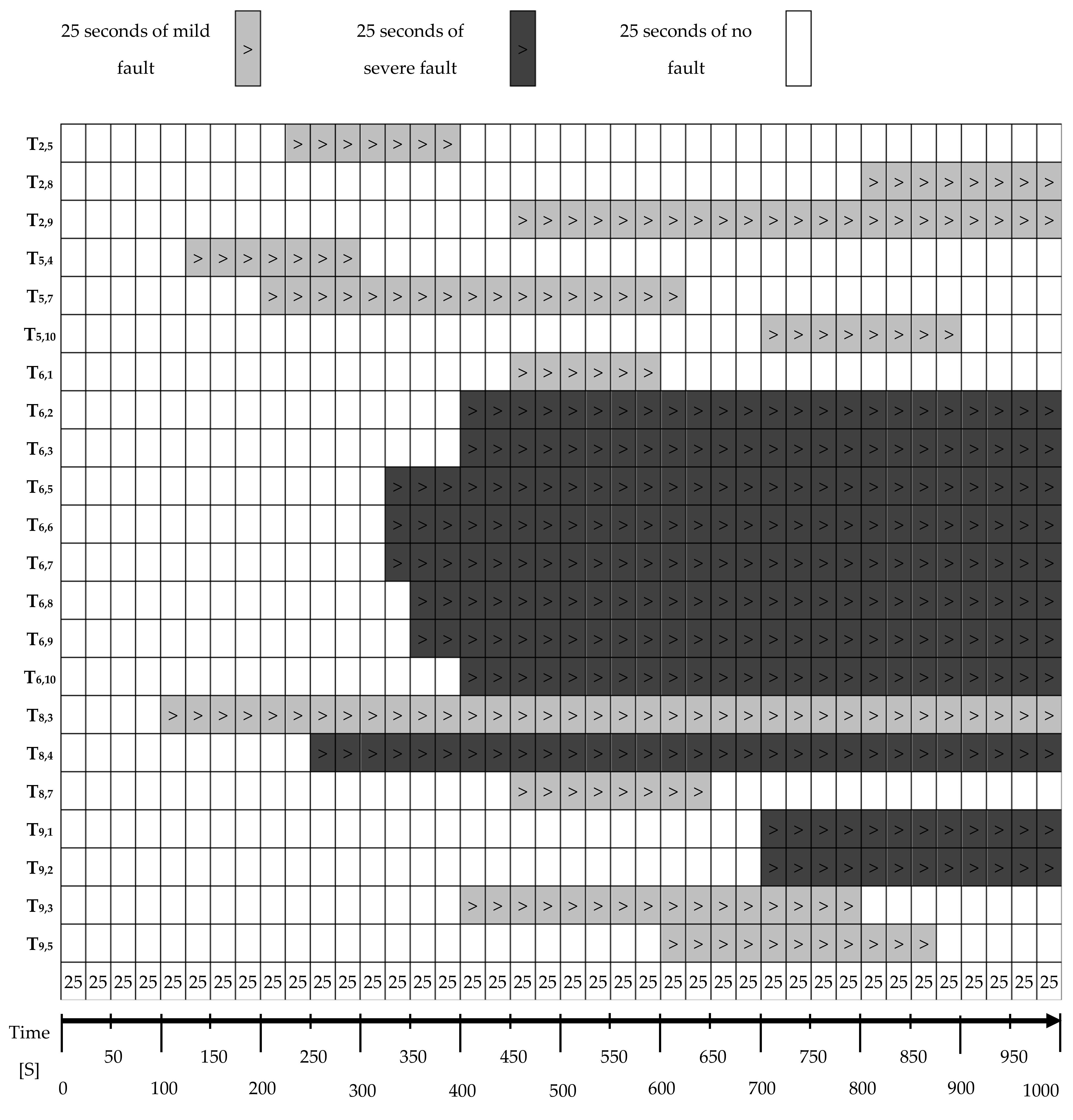
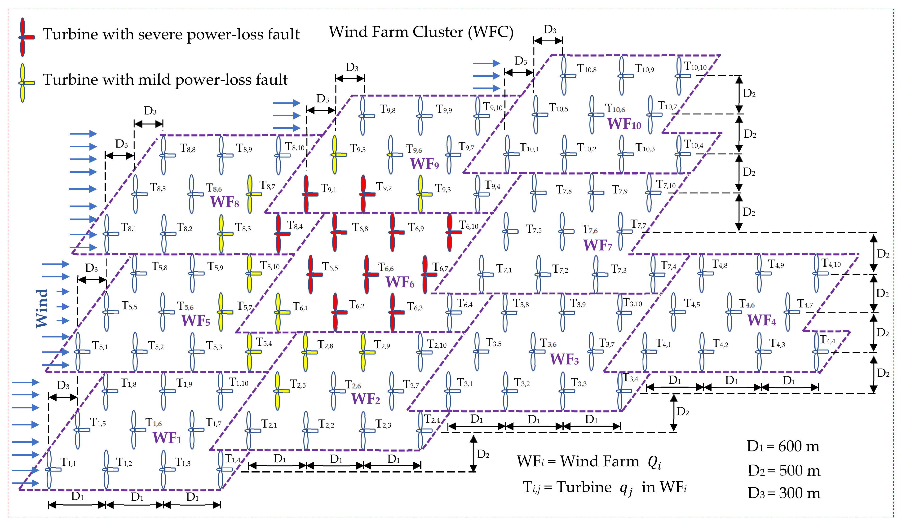
4. Simulation Results

The nonlinear benchmark model for WFC and the power loss faults in Section 2 are used here to evaluate the effectiveness and performance of the proposed active FTCC scheme. The considered power loss faults are mathematically modelled through scaling the output powers of faulty wind turbines, representing their decreased power generation. In reference to the WFC of 100 wind turbines shown in Figure 1, a typical fault scenario is designed for a total simulation time of 1000 s during which mild and severe power loss faults occur in some wind turbines. Among the said faults it is assumed that some simultaneously occur in more than one wind turbine. The timeline for the occurrence of mild and severe faults in a designated number of wind turbines in the WFC is shown in Figure 8. Figure 9 illustrates the layout of the WFC under the considered faults.

For wind farms $Q_2$ and $Q_5$ (i.e., $W{F}_2$ and $W{F}_5$ in Figure 9) that are only impacted by mild power loss faults, no control reallocation at wind farm or WFC levels would be necessary (see Algorithms 1 and 2). Indeed, the previously discussed ASC mechanism at wind turbine level is adequate to automatically accommodate mild faults effects. However, for wind farms $Q_8$ and $Q_9$ (i.e., $W{F}_8$ and $W{F}_9$ in Figure 9), the procedure is similar to wind farms $Q_2$ and $Q_5$ except for $T_{8,4}$, $T_{9,1}$, and $T_{9,2}$ that are impaired by severe power loss faults. The magnitude of such faults in the mentioned severely faulty turbines develops to a severe total power loss as shown in Figure 10. In general, a total power loss condition can occur either because of a shutdown command by the farm operator or an unpredicted failure. However, the proposed active FTCC scheme accommodates the adverse impacts of any severe power loss faults (no matter partial or total). As per Algorithm 1, severe power loss effects in faulty wind farms $Q_8$ and $Q_9$ can be accommodated by farm-level control reallocation. In addition, ASC at the turbine level still accommodates the remaining impacts of mild power loss faults in $T_{8,3}$, $T_{8,7}$, $T_{9,3}$, and $T_{9,5}$. Unlike the previously discussed cases, for wind farm $Q_6$ (i.e., $W{F}_6$ in Figure 9), the fault accommodation at the wind turbine or wind farm level will not be effective (due to the number of severely faulty wind turbines and the lack of enough available power in the farm (see Figure 9 and Figure 10)). Therefore, the control commands must be reallocated among the wind farms at WFC level as per Algorithm 2. The following subsections provide more information about the conducted simulation results.

4.1. Mild Power Loss Fault Accommodation at the Turbine Level

In reference to fault-accommodation at the turbine level in wind farms $Q_2$ and $Q_5$, Figure 11 shows the generated power during fault-free (nominal) and faulty operations with or without considering the FTCC scheme. As shown by the black lines (i.e., faulty operation with FTCC scheme) following the green lines (i.e., nominal operation), the proposed FTCC scheme (i.e., FDD integrated with ASC at turbine level) can effectively accommodate the faults effects. In addition, this figure illustrates that the FTCC scheme under fault-free operation has almost no effects on the performance of the wind turbines. To demonstrate clearly, Figure 11 only shows generated power around the faults’ activity periods in the turbines with considered mild faults. Similarly, for the other turbines impacted by mild power loss faults in wind farms $Q_6$, $Q_8$ and $Q_9$ (i.e., $W{F}_6$, $W{F}_8$ and $W{F}_9$ in Figure 9), the corresponding ASC units (i.e., ASC units 6, 8 and 9 integrated with FDD systems 6, 8 and 9, respectively) accommodate the faults impacts at wind turbine level.

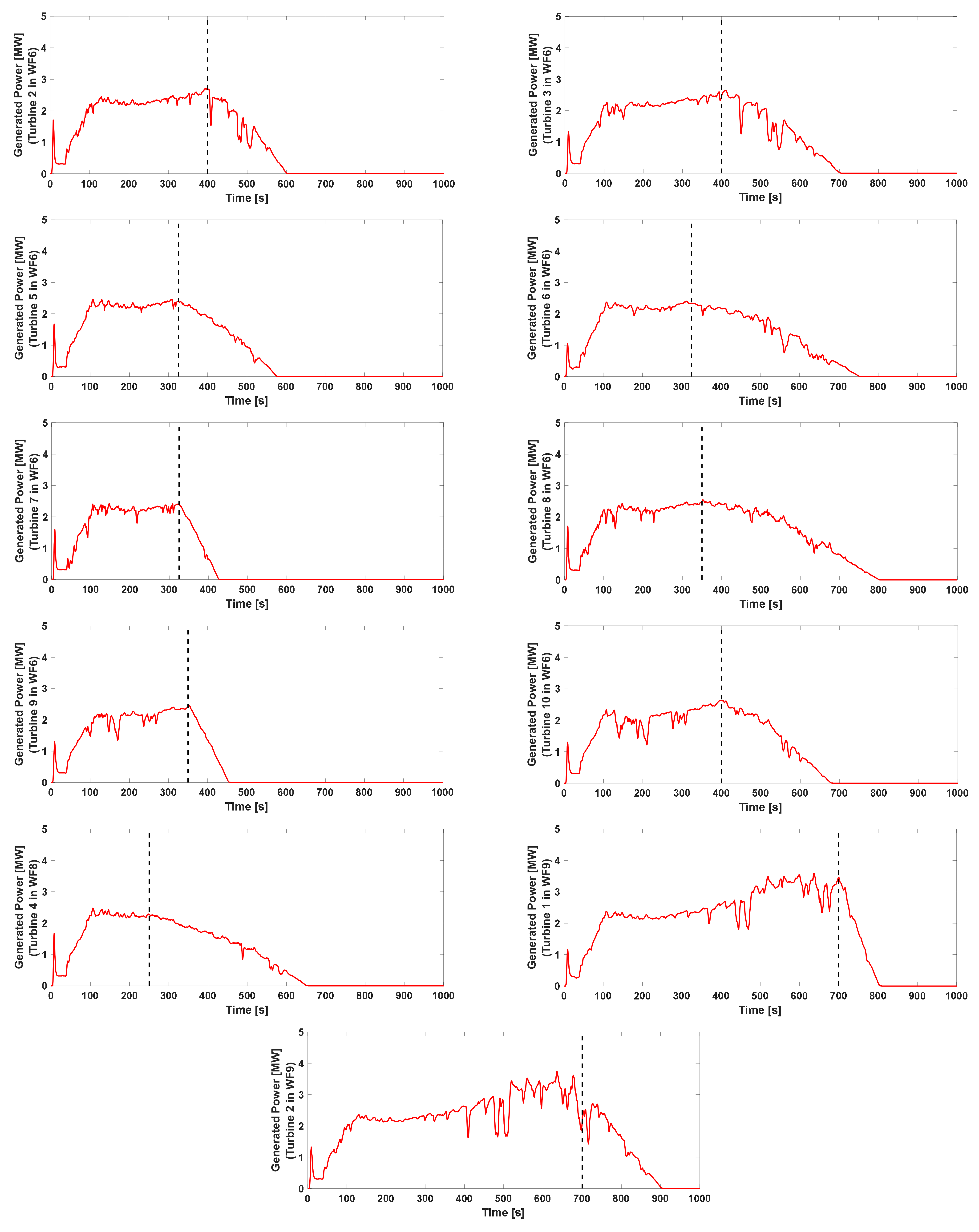
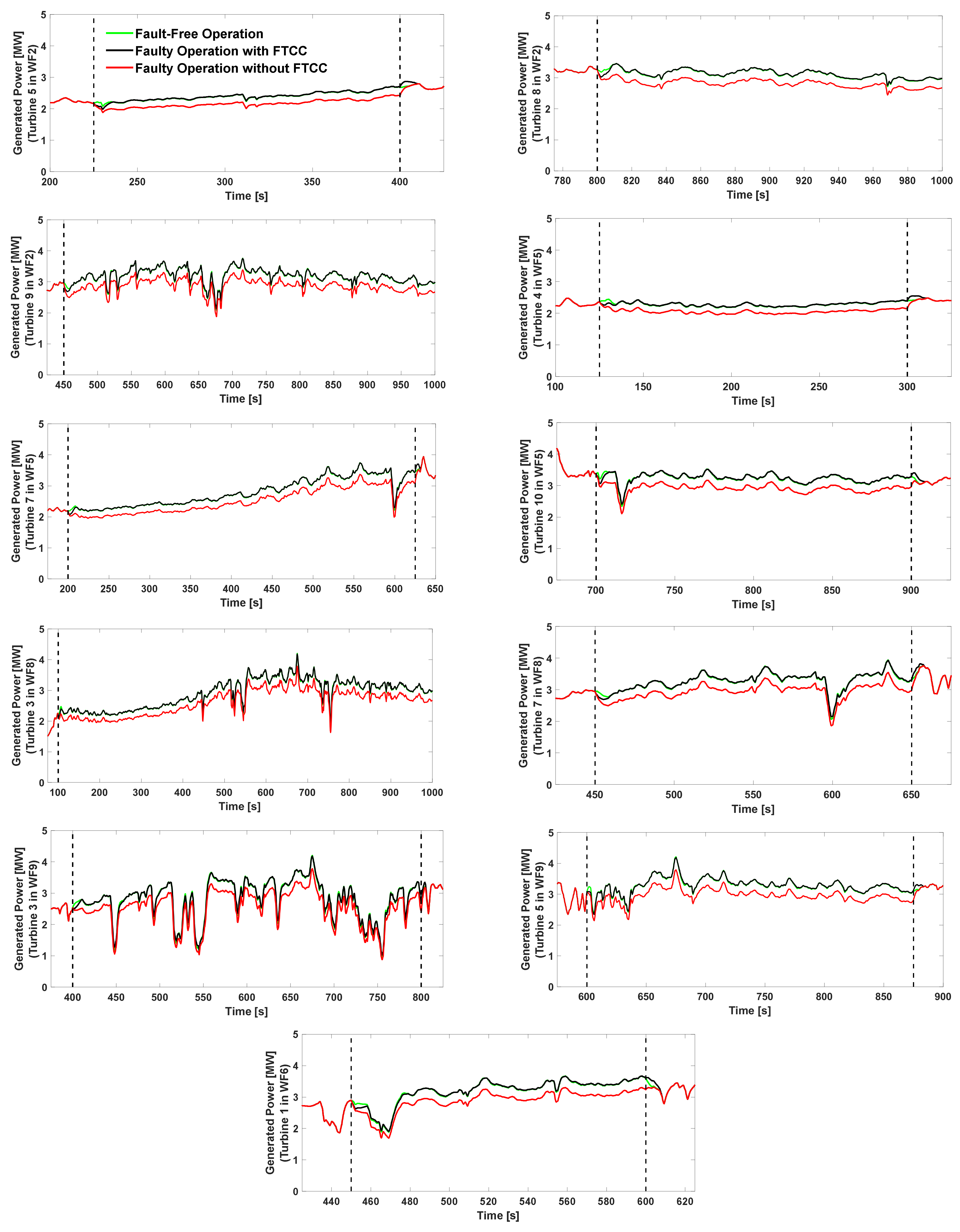
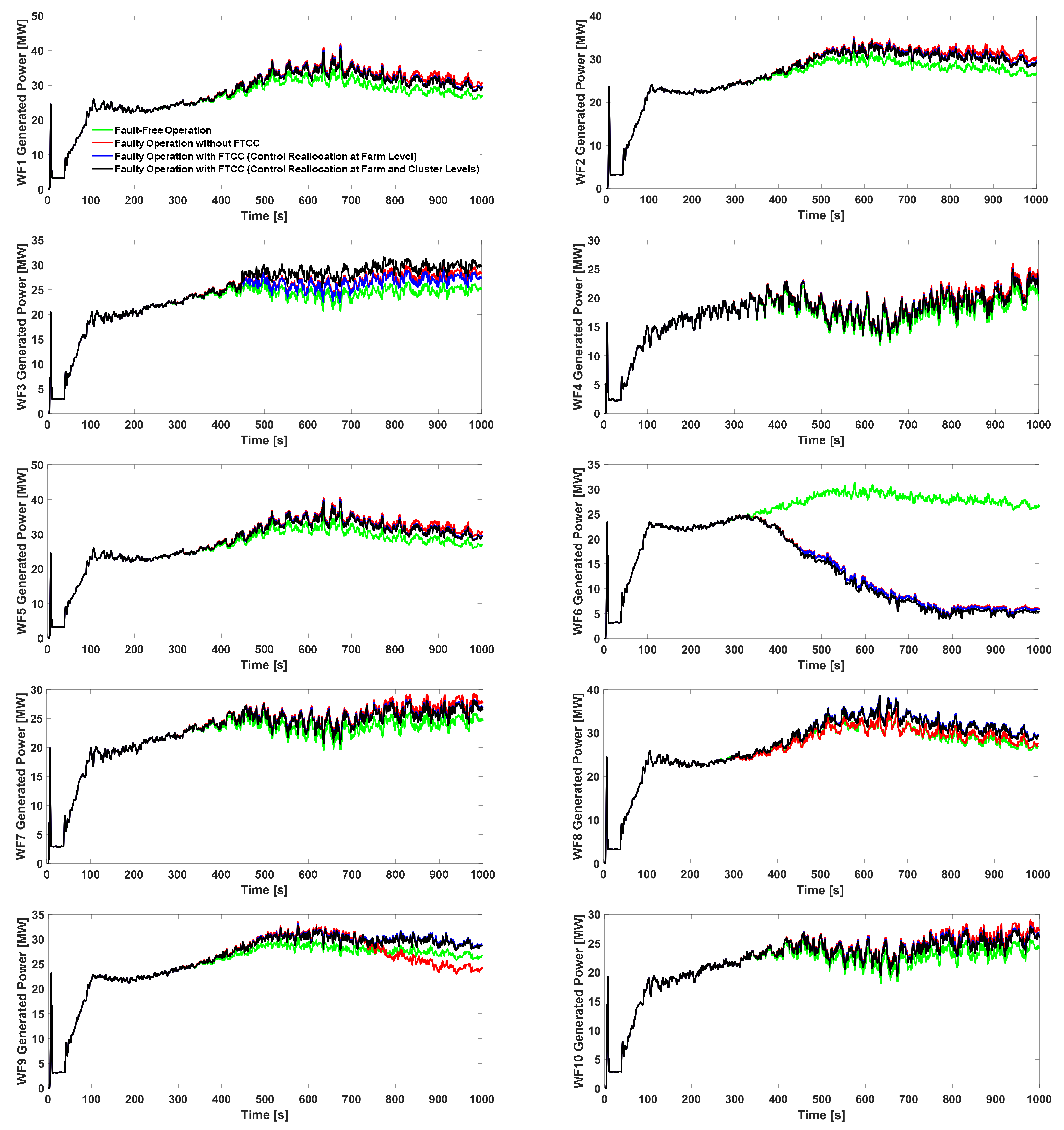
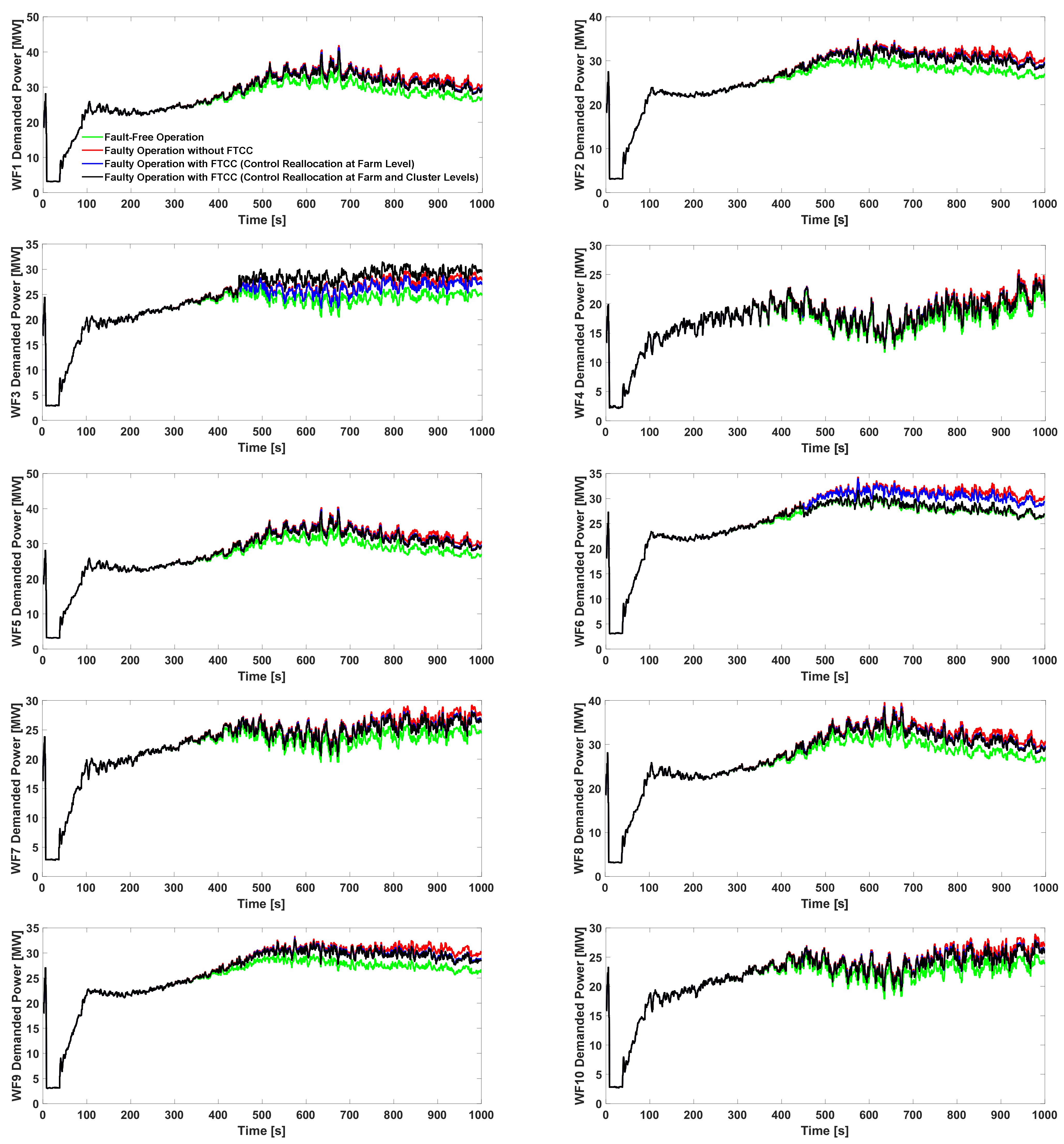
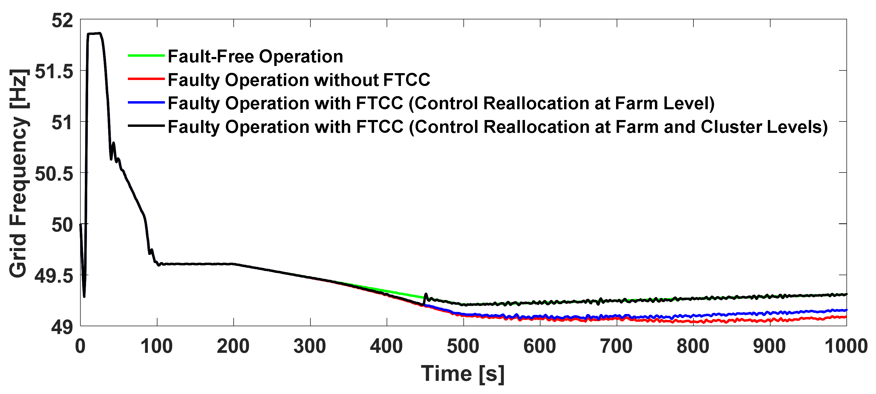
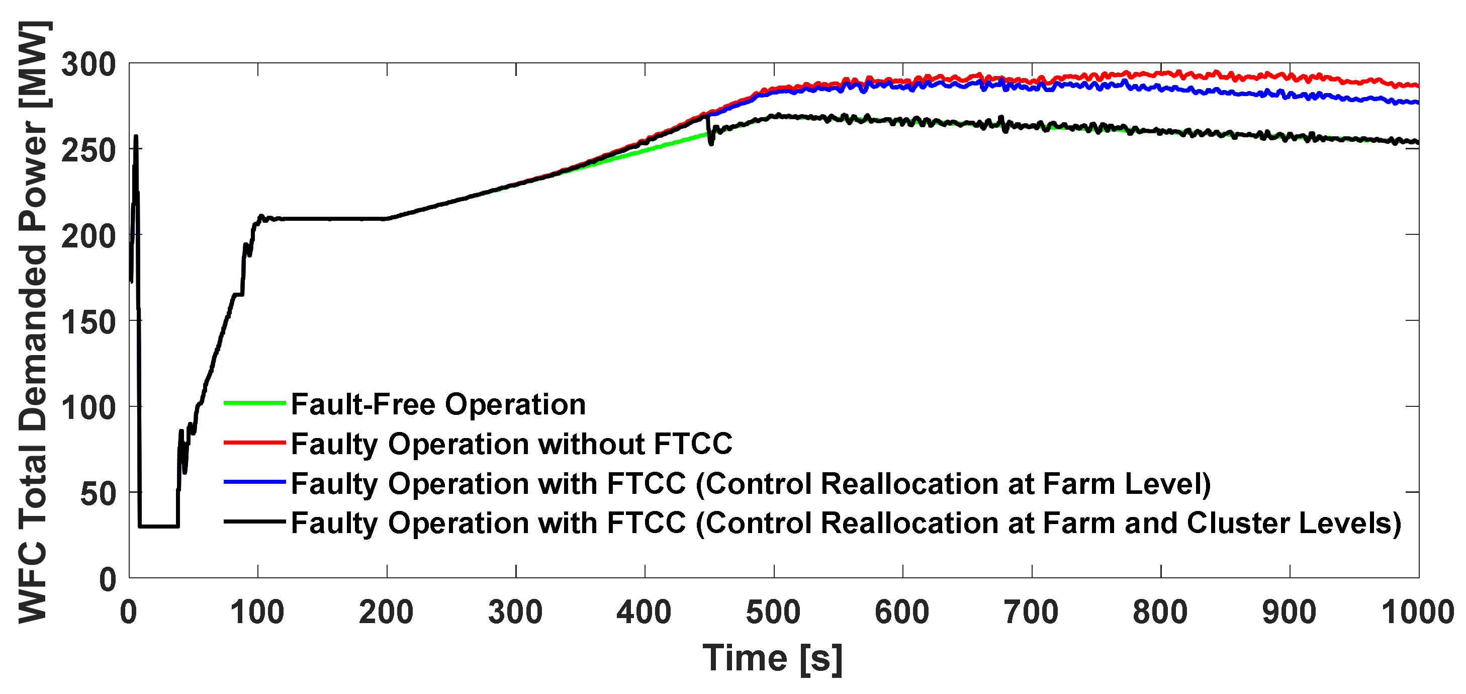
4.2. Severe Power Loss Fault Accommodation at Farm and Cluster Levels

As per already depicted fault scenario in Figure 8, some wind turbines in farms $Q_6$, $Q_8$, and $Q_9$ encounter severe power loss faults. Specifically, the severe fault effects in wind farms $Q_8$ and $Q_9$ are accommodated by the farm-level control reallocation mechanism based on Algorithm 1 since there is enough available power in the farms’ healthy wind turbines.

However, for the accommodation of severe fault effects in farm $Q_6$, the farm-level control reallocation is not sufficient due to the lack of enough available power in the farm’s healthy wind turbines (i.e., ${\mathrm{T}}_{6,1}$ and ${\mathrm{T}}_{6,4}$). Therefore, the entire active FTCC scheme, including the WFC-level control reallocation (Algorithm 2), automatically tackles severe fault effects in addition to the other mild fault effects.

In Figure 12, comparing the generated powers in wind farms during fault-free (nominal) and faulty operations with and without the active FTCC scheme, it is observed that the faulty operations (for the same wind farms) with farm-level control reallocation (blue lines) are different from the faulty operations with both farm-level and WFC-level control reallocations (black lines). This is due to the severe power loss faults in $Q_6$, changing $H{F}_{Q_6}$ to zero (at about 450 sec), which activates the WFC-level control reallocation mode to compensate the total missed power in $Q_6$. The resultant control commands are obviously different. This fact is also seen in Figure 13 that shows the demanded powers sent by the network operator to the respective wind farms in the cluster. As seen, the power demanded from $Q_6$ (severely impaired wind farm) is almost the same as that under nominal operation. However, for the healthy wind farms, the demanded power is increased to accommodate the overall fault effects at the cluster level.

The WFC’s characteristics, including the grid frequency and the total active power (tracking the considered grid load), are illustrated in Figure 14 and Figure 15, respectively. In these figures, the adverse fault impacts (because of severe power loss faults) are clearly observed as significant deviations in the grid frequency response and total generated power (compare the red lines with the green lines in the figures). However, the black lines (i.e., faulty operation with active FTCC) in the figures show that the proposed active FTCC scheme successfully accommodates the adverse fault effects at the farm and cluster levels. The observed fluctuations in the black lines correspond to the moments of major disturbances in the wind speed or the occurrence of mild power loss faults. As can be seen, the proposed active FTCC scheme can handle all the mentioned moments effectively.

Moreover, the blue lines in Figure 14 and Figure 15 indicate faulty operation with the active FTCC scheme but by ASC and farm-level control reallocation only. Predictably, the accommodation of considered power loss faults still enhances the grid frequency response but not as efficiently as with the complete active FTCC scheme that accommodates the severe faults at the cluster level.

As seen in Figure 16, illustrating the total demanded power from the WFC during fault-free (nominal) and faulty operations with or without FTCC, the WFC under faulty operation without active FTCC is required to provide more power than the same WFC but with active FTCC. Indeed, the total demanded power under faulty operation with active FTCC is almost similar to that under fault-free operation. The faulty operation with the active FTCC scheme (black line in Figure 16) shows that at about 450 s, the network operator automatically switches to the control reallocation mode.

Finally, to evaluate the robustness of the proposed FTCC scheme against measurement uncertainties and communication delays, extensive Monte Carlo simulations were performed. In the considered benchmark model, sensors (i.e., anemometer, rotor speed, generator speed, and blade pitch angle sensors) are considered as noise-contaminated measurement systems, and communication links between network operator and wind farm controllers, and between each wind farm controller and its corresponding turbines, contain time delays. The measurement noises in each sensor and the time delay in each communication link are generated as band-limited white noise.

Table 4. Available sensors and their white noise parameters.

Sensor	Unit	Noise Power		Starting Seed
		Nominal	Error
Anemometer—Wind speed at hub height	m/s	$0.006$	$50\%$	Stochastic values
Rotor speed	rad/s	$0.0001$
Generator speed	rad/s	$0.0002$
Blade pitch angle	deg	$0.0012$

and

Table 5. Considered communication links and their white noise parameters.

Communication Link	Delay		Starting Seed
	Nominal	Error
Between network operator and wind farm controllers in WFC	$0.1$ s	$50\%$	Stochastic values
Between wind farm controller and turbines in each wind farm	$0.01$ s

present the considered sensors and communication links with relevant parameters used during the simulations. Overall, 100 Monte Carlo simulations were performed for the designed FTCC scheme.

Table 6. Results of Monte Carlo simulation studies for severe power loss fault scenario.

Severe Faults (Farm and Cluster Levels)	Results	Active FTCC
		Switching Time 1 (s)	RMSPE 2 (%)
WF8	Best Case	312.9	0.267
	Average Case	313.2	0.295
	Worst Case	313.4	0.310
WF9	Best Case	707.8	0.412
	Average Case	708.1	0.435
	Worst Case	708.2	0.490
WFC	Best Case	447	0.295
	Average Case	448	0.321
	Worst Case	449	0.382

¹ Switching time from normal operation to reallocation mode in wind farm controllers and network operator. ² Root-Mean-Squared-Percentage Error (RMSPE). Note: The RMSPE is calculated with respect to the generated power in farms $W{F}_8$ and $W{F}_9$, and total generated power in WFC.

and

Table 7. Results of Monte Carlo simulation studies for mild power loss fault scenario.

Mild Faults (Turbine Level)	Results	Active FTCC
		Detection Time 1 (s)	RMSPE (%)
T2,5	Best Case	1.58	0.204
	Average Case	1.69	0.318
	Worst Case	1.91	0.402
T2,8	Best Case	1.51	0.198
	Average Case	1.73	0.267
	Worst Case	2.05	0.396
T2,9	Best Case	1.89	0.211
	Average Case	2.10	0.304
	Worst Case	2.61	0.435
T5,4	Best Case	1.91	0.283
	Average Case	2.12	0.315
	Worst Case	2.54	0.333
T5,7	Best Case	2.05	0.326
	Average Case	2.67	0.409
	Worst Case	3.23	0.455
T5,10	Best Case	2.61	0.275
	Average Case	3.19	0.331
	Worst Case	3.66	0.395
T6,1	Best Case	1.95	0.230
	Average Case	2.15	0.353
	Worst Case	2.42	0.406
T8,3	Best Case	1.52	0.215
	Average Case	1.90	0.253
	Worst Case	2.44	0.301
T8,7	Best Case	2.85	0.320
	Average Case	3.03	0.442
	Worst Case	3.54	0.525
T9,3	Best Case	2.41	0.353
	Average Case	2.83	0.441
	Worst Case	3.09	0.510
T9,5	Best Case	1.28	0.203
	Average Case	1.35	0.233
	Worst Case	1.51	0.281

¹ Fault detection time obtained from FDD system. Note that the RMSPE is calculated with respect to the generated power in each wind turbine with mild-power loss fault.

provide the best, average, and worst values of the performance characteristics obtained from the simulations for severe and mild power loss fault scenarios, respectively. In summary, all the simulation results confirm that the proposed active FTCC scheme can successfully maintain reliable wind farm and WFC performance under faulty conditions and in the presence of possible uncertainties.

5. Conclusions and Future Works

This paper proposes and addresses the design, development, and structure of a novel active fault-tolerant cooperative control (FTCC) scheme for large-scale wind farms and wind farm clusters (WFCs). This active FTCC scheme tackles common power loss faults in wind turbines from mild to severe power loss even total failure, all of which may be due to different levels of icing or debris build-up on turbine’s rotor blades. To accommodate the effects of mild faults at turbine level, the active FTCC scheme employs automatic signal correction (ASC) units integrated with distributed fault detection and diagnosis (FDD) systems in each wind farm of the cluster. However, to accommodate the effects of severe faults, the active FTCC scheme uses a two-layer hierarchical control reallocation mechanism at the wind farm and wind farm cluster levels. This needs healthier turbines/farms (with an extra available power) to compensate the missing (pending) power from severely impacted turbines/farms by producing stable and reliable power even in the presence of different levels of faults.

Various simulation studies on an advanced WFC benchmark model indicate the high effectiveness of the proposed schemes and solutions over an entire range of considered wind profiles and in the presence of wind profile turbulences, possible measurement noises and other realistic fault scenarios. The noticeable fault-tolerance capability obtained by the active FTCC scheme makes it superior to a typical WFC control system. The fact that the proposed scheme employs a type of signal correction technique makes it more industry-friendly compared to other methods cited in the technical literature. Moreover, the active FTCC scheme addresses off-normal power reductions due to both partial and total power loss conditions. This is done without interfering with the main duties of a WFC operator, including the shutdown of the turbines with severe power loss. In addition to the mentioned benefits, the proposed active FTCC scheme requires less computational power compared with the previous methods, since the proposed clustering approach in the scheme reduces the number of modules needed for computations significantly. However, future research should investigate for how long a severely faulty turbine is prescribed to continue working and contribute to farm power production before being structurally endangered. Different control techniques at each level (i.e., turbine, farm, and cluster levels) as well as passive FTCC approaches can also be investigated. Finally, when clustering a very large-scale wind farm, determining the optimal sizes of small-scale wind farms before activating the control reallocation mechanism at network operator level is another interesting topic that remains for future work.

References

1. Sloth, C.; Esbensen, T.; Stoustrup, J. Robust and Fault-Tolerant Linear Parameter-Varying Control of Wind Turbines. Mechatronics 2011, 21, 645–659. [Google Scholar] [CrossRef] [Green Version]
2. Tabatabaeipour, S.M.; Odgaard, P.F.; Bak, T.; Stoustrup, J. Fault Detection of Wind Turbines with Uncertain Parameters: A Set-Membership Approach. Energies 2012, 5, 2424–2448. [Google Scholar] [CrossRef] [Green Version]
3. Simani, S.; Castaldi, P. Active Actuator Fault-Tolerant Control of a Wind Turbine Benchmark Model. Int. J. Robust Nonlinear Control 2014, 24, 1283–1303. [Google Scholar] [CrossRef] [Green Version]
4. Badihi, H.; Zhang, Y.M.; Hong, H. Fuzzy Gain-Scheduled Active Fault-Tolerant Control of a Wind Turbine. J. Frankl. Inst. 2014, 351, 3677–3706. [Google Scholar] [CrossRef]
5. Fekih, A.; Mobayen, S.; Chen, C.C. Adaptive Robust Fault-Tolerant Control Design for Wind Turbines Subject to Pitch Actuator Faults. Energies 2021, 14, 1791. [Google Scholar] [CrossRef]
6. Mazare, M.; Taghizadeh, M.; Ghaf-Ghanbari, P. Fault Tolerant Control of Wind Turbines with Simultaneous Actuator and Sensor Faults using Adaptive Time Delay Control. Renew. Energy 2021, 174, 86–101. [Google Scholar] [CrossRef]
7. Badihi, H.; Zhang, Y.M.; Hong, H. Wind Turbine Fault Diagnosis and Fault-Tolerant Torque Load Control against Actuator Faults. IEEE Trans. Control Syst. Technol. 2015, 23, 1351–1372. [Google Scholar] [CrossRef]
8. Gao, Z.; Liu, X. An Overview on Fault Diagnosis, Prognosis and Resilient Control for Wind Turbine Systems. Processes 2021, 9, 300. [Google Scholar] [CrossRef]
9. Badihi, H.; Zhang, Y.M.; Pillay, P.; Rakheja, S. Fault-Tolerant Individual Pitch Control for Load Mitigation in Wind Turbines with Actuator Faults. IEEE Trans. Ind. Electron. 2021, 68, 532–543. [Google Scholar] [CrossRef]
10. Kusiak, A.; Verma, A. A Data-Driven Approach for Monitoring Blade Pitch Faults in Wind Turbines. IEEE Trans. Sustain. Energy 2011, 2, 87–96. [Google Scholar] [CrossRef]
11. Kusiak, A.; Verma, A. A Data-Mining Approach to Monitoring Wind Turbines. IEEE Trans. Sustain. Energy 2012, 3, 150–157. [Google Scholar] [CrossRef]
12. Wang, Y.; Ma, X.; Qian, P. Wind Turbine Fault Detection and Identification through PCA-Based Optimal Variable Selection. IEEE Trans. Sustain. Energy 2018, 9, 1627–1635. [Google Scholar] [CrossRef] [Green Version]
13. Marvuglia, A.; Messineo, A. Monitoring of Wind Farms’ Power Curves using Machine Learning Techniques. Appl. Energy 2012, 98, 574–583. [Google Scholar] [CrossRef]
14. Karamichailidou, D.; Kaloutsa, V.; Alexandridis, A. Wind Turbine Power Curve Modeling Using Radial Basis Function Neural Networks and Tabu Search. Renew. Energy 2021, 163, 2137–2152. [Google Scholar] [CrossRef]
15. Blesa, J.; Jiménez, P.; Rotondo, D.; Nejjari, F.; Puig, V. An Interval NLPV Parity Equations Approach for Fault Detection and Isolation of a Wind Farm. IEEE Trans. Ind. Electron. 2015, 62, 3794–3805. [Google Scholar] [CrossRef] [Green Version]
16. Badihi, H.; Zhang, Y.M.; Hong, H. Active Fault Tolerant Control in a Wind Farm with Decreased Power Generation due to Blade Erosion/Debris Build-Up. IFAC-Pap. 2015, 48, 1369–1374. [Google Scholar] [CrossRef]
17. Li, D.; Li, P.; Cai, W.; Song, Y.; Chen, H. Adaptive Fault-Tolerant Control of Wind Turbines with Guaranteed Transient Performance Considering Active Power Control of Wind Farms. IEEE Trans. Ind. Electron. 2018, 65, 3275–3285. [Google Scholar] [CrossRef]
18. Ma, K.; Zhu, J.; Soltani, M.; Hajizadeh, A.; Chen, Z. Optimal Power Dispatch of an Offshore Wind Farm under Generator Fault. Appl. Sci. 2019, 9, 1184. [Google Scholar] [CrossRef] [Green Version]
19. Ma, K.; Soltani, M.; Hajizadeh, A.; Zhu, J.; Chen, Z. Wind Farm Power Optimization and Fault Ride-Through under Inter-Turn Short-Circuit Fault. Energies 2021, 14, 3072. [Google Scholar] [CrossRef]
20. Badihi, H.; Zhang, Y.M.; Hong, H. Fault-Tolerant Cooperative Control in an Offshore Wind Farm using Model-Free and Model-Based Fault Detection and Diagnosis Approaches. Appl. Energy 2017, 201, 284–307. [Google Scholar] [CrossRef]
21. Badihi, H.; Zhang, Y.M.; Pillay, P.; Rakheja, S. Application of FMRAC to Fault-Tolerant Cooperative Control of a Wind Farm with Decreased Power Generation due to Blade Erosion/Debris Build-Up. Int. J. Adapt. Control. Signal Process. 2018, 32, 628–645. [Google Scholar] [CrossRef]
22. Badihi, H.; Jadidi, S.; Zhang, Y.M.; Pillay, P.; Rakheja, S. Fault-Tolerant Cooperative Control in a Wind Farm using Adaptive Control Reconfiguration and Control Reallocation. IEEE Trans. Sustain. Energy 2019, 11, 2119–2129. [Google Scholar] [CrossRef]
23. Soltani, M.; Knudsen, T.; Bak, T. Modeling and Simulation of Offshore Wind Farms for Farm Level Control. In Proceedings of the European Offshore Wind Conference and Exhibition (EOW), Stockholm, Sweden, 15 September 2009. [Google Scholar]
24. Jonkman, J.; Butterfield, S.; Musial, W.; Scott, G. Definition of a 5 MW Reference Wind Turbine for Offshore System Development; National Renewable Energy Laboratory: Golden, CO, USA, 2009. [Google Scholar]
25. Jadidi, S.; Badihi, H.; Zhang, Y.M. A Review on Operation, Control and Protection of Smart Microgrids. In Proceedings of the IEEE 2nd International Conference on Renewable Energy and Power Engineering (REPE), Toronto, ON, Canada, 2–4 November 2019; pp. 100–104. [Google Scholar] [CrossRef]
26. Fingersh, L.; Carlin, P. Results from the NREL Variable-Speed Test Bed. In Proceedings of the 17th ASME Wind Energy Symposium, Reno, NV, USA, 12 January 1998; pp. 233–237. [Google Scholar] [CrossRef] [Green Version]
27. Johnson, K.E.; Pao, L.Y.; Balas, M.J.; Fingersh, L.J. Control of Variable-Speed Wind Turbines: Standard and Adaptive Techniques for Maximizing Energy Capture. IEEE Control. Syst. Mag. 2006, 26, 71–81. [Google Scholar] [CrossRef]
28. Jadidi, S.; Badihi, H.; Zhang, Y.M. Passive Fault-Tolerant Control Strategies for Power Converter in a Hybrid Microgrid. Energies 2020, 13, 5625. [Google Scholar] [CrossRef]
29. Jadidi, S.; Badihi, H.; Zhang, Y.M. Passive Fault-Tolerant Control of PWM Converter in a Hybrid AC/DC Microgrid. In Proceedings of the IEEE 2nd International Conference on Renewable Energy and Power Engineering (REPE), Toronto, ON, Canada, 2–4 November 2019; pp. 90–94. [Google Scholar] [CrossRef]
30. Zhang, Y.M.; Jiang, J. Bibliographical Review on Reconfigurable Fault-Tolerant Control Systems. Annu. Rev. Control. 2008, 32, 229–252. [Google Scholar] [CrossRef]
31. Babuska, R. Fuzzy Modeling for Control; Springer: Berlin/Heidelberg, Germany, 1998. [Google Scholar]
Figure 1. Layout of the considered wind farm cluster (WFC) benchmark model.
Energies 14 07436 g001
Figure 2. Block diagram of the wind farm cluster (WFC) benchmark model ( N = 10 and N i = 10 ).
Energies 14 07436 g002
Figure 3. External view of the active FTCC control-loop with other distributed components in the WFC benchmark model.
Energies 14 07436 g003
Figure 4. Architecture of the proposed fault-tolerant cooperative controller (FTCC) and distributed FDD system for the WFC.
Energies 14 07436 g004
Figure 5. FDD system i for wind farm Q i with N i wind turbines. Each module M (from R i modules) monitors the consistency of generated powers from any two specific wind turbines in the wind farm. The module outputs, denoted by M O with appropriate subscripts, are analyzed and final decisions are made by the relevant decision making ( D M ) processes. Note that, q Z with ( Z and 1 < Z < N i ) represents any wind turbine except q 1 and q N i .
Energies 14 07436 g005
Figure 6. Example module M α , β .
Energies 14 07436 g006
Figure 7. The internal structure of module M α , β based on [20].
Energies 14 07436 g007
Figure 8. Timeline for the occurrence of power loss faults in the considered wind turbines in the cluster. The simulation time is 1000 s. T# indicates turbine number according to the WFC layout in Figure 9.
Energies 14 07436 g008
Figure 9. Layout of the wind farm cluster under considered fault scenario.
Energies 14 07436 g009
Figure 10. Generated power from respective wind turbines with severe power loss faults.
Energies 14 07436 g010
Figure 11. Generated power from respective wind turbines impacted by mild power loss faults during fault-free and faulty operations.
Energies 14 07436 g011
Figure 12. Generated power from each wind farm in the WFC under fault-free (nominal) and faulty operations with and without active FTCC.
Energies 14 07436 g012
Figure 13. Demanded power from the wind farms of the WFC under fault-free (nominal) and faulty operations.
Energies 14 07436 g013
Figure 14. Grid frequency during fault-free and faulty operations.
Energies 14 07436 g014
Figure 15. WFC total generated power.
Energies 14 07436 g015
Figure 16. Total demanded power from the WFC.
Energies 14 07436 g016