Numerical and Experimental Investigation of Wire Cloth Heat Exchanger for Latent Heat Storages

Abstract

Latent thermal energy storages (LTES) offer a high storage density within a narrow temperature range. Due to the typically low thermal conductivity of the applied phase change materials (PCM), the power of the storages is limited. To increase the power, an efficient heat exchanger with a large heat transfer surface and a higher thermal conductivity is needed. In this article, planar wire cloth heat exchangers are investigated to obtain these properties. They investigated the first time for LTES. Therefore, we developed a finite element method (FEM) model of the heat exchanger and validated it against the experimental characterization of a prototype LTES. As PCM, the commercially available paraffin RT35HC is used. The performance of the wire cloth is compared to tube bundle heat exchanger by a parametric study. The tube diameter, tube distance, wire diameter and heat exchanger distance were varied. In addition, aluminum and stainless steel were investigated as materials for the heat exchanger. In total, 654 variants were simulated. Compared to tube bundle heat exchanger with equal tube arrangement, the wire cloth can increase the mean thermal power by a factor of 4.20 but can also reduce the storage capacity by a minimum factor of 0.85. A Pareto frontier analysis shows that for a free arrangement of parallel tubes, the tube bundle and wire cloth heat exchanger reach similar performance and storage capacities.

1. Introduction

Thermal energy storages are required wherever a discrepancy between demand and availability of thermal energy occurs. There is a wide range of applications with different operational temperatures like heat and cold supply for buildings, industrial processes and thermal power plants. As common technology sensible thermal storages are used. The main drawback is the implied temperature change of the storage material during operation leading to reduced process efficiency. Latent thermal energy storages (LTES) overcome this drawback by phase change materials (PCM) as storage material. By the utilization of a phase change, a narrow temperature variation of the storage and a high storage density is possible. Commonly, a material with solid–liquid phase change is chosen due to low volume change in the phase transition [1]. One of the main drawbacks of PCM is the low thermal conductivity limiting the heat transfer and thus the thermal power of latent heat storages [1]. This can be compensated by an efficient heat exchanger immersed in the PCM, which is passed by a conventional heat transfer fluid (HTF). The heat exchanger requires a high thermal conductivity and heat transfer surface area within the PCM volume. Furthermore, a low volume fraction of the heat exchanger is needed to retain the high storage density. Besides the performance parameters, the compatibility between PCM and the heat exchanger, the operation temperature and the pressure drop need to be considered for the design.

So far, there is no standard heat exchanger for LTES. An overview of the different technologies is given by the reviews from Jegadheeswaran et al. [2], Khan et al. [3] and Liu et al. [4]. One possibility are plate heat exchangers. Multiple heat exchanger plates passed by a HTF are arranged in parallel while PCM is located in between the plates. Neumann et al. developed validated models for parallel arranged aluminum roll-bond plates with bionically inspired FracTherm^® HTF channel structure, developed by Fraunhofer ISE [5]. Saeed et al. investigated roll-bond plates under different arrangements and operation conditions [6]. It was found that performance is increased by smaller plate distance, higher mass flow rate and higher temperature differences. Johnson et al. used a flat plate heat exchanger with and without additional heat transfer enhancement structures [7,8]. The charge and discharge time was significantly reduced by enhancement structures.

Much more common than plate heat exchangers are finned tube heat exchangers. Agyenim compared the performance of circular and longitudinal fins to a bare tube [9]. The different geometries were rated according to the temperature evolution and charging time. It was found that longitudinal fins enhance the performance more than circular. Gil et al. also investigated tube and finned tube heat exchanger [10,11]. Laing et al. studied tubes with fins made from aluminum and graphite [12]. The graphite fins performed better but were only stable below 250 °C. For higher temperatures the aluminum fins were preferred. Neumann et al. as well as Anish et al. characterized experimentally the finned tube heat exchanger [13,14]. Rahimi et al. investigated the influence of fin spacing on performance [15]. They observed a significantly reduced phase change duration using fins. When the fin distance was smaller, the duration was further shortened. Kabbara et al. characterized experimentally hydronic baseboard space-heating radiator finned tubes because of their low-cost production under different operation conditions [16]. With higher temperature difference and mass flow rates, a reduced charging time was achieved. Tay et al. investigated a bare tube heat exchanger and did a comparison with pin and radial fins [17,18]. It was noted that radial fins increase the performance more than pin fins. Hejčík theoretically investigated polymeric hollow fibers with inner diameters between 0.5 and 1.5 mm as an alternative to metal tubes [19]. The polymeric fibers can be easily produced by extrusion processes and do not suffer from corrosion like metallic tubes. The performance was better for reduced diameters but the required pump power increases.

Besides fins, the heat transfer can also be enhanced by metal foams arranged around heat exchanger tubes. Yang et al. compared tube, finned tube, tube with foams as well as finned tubes with foam [20]. The foams were made of copper. The highest performance was reached by the combination of fins and foam. By a porosity of 97%, the foams still allowed a high PCM content. Wang et al. investigated the difference of homogeneous and gradient porosity copper foam [21]. The porosity was increased with distance to the heat exchanger tube. With gradient porosity foam the heat transfer rate was increased and the melting time was reduced by 37.6% compared to homogenous porosity foam.

A further alternative for heat transfer enhancement is the use of wire structures. Youssef et al. investigated a spiral-wired tube heat exchanger [22]. Tubes with 22 mm diameter were used. The wires were soldered perpendicular to the tube surface. Khan et al. compared wire-wounded fins to longitudinal and radial fins [23]. The discharge time was reduced by 68% and 25% compared to the longitudinal and radial fins, respectively. Spiral wounded wire structures were numerically evaluated by Schlott et al. [24]. It was shown that for increased power the thermal conductivity of the wire and the interconnection between the wires is important. Koller et al. investigated numerically an aluminum wire matrix around a single tube numerically [25]. Besides metallic wires, carbon fibers have also been tested. Nakaso et al. used a tube heat exchanger and snaked carbon fiber cloth from tube to tube [26]. Additionally, they tested fiber brushes around the tubes. Compared to the brushes with the cloth, the same power was achieved but with less volume fraction of fibers.

A comparison of different heat exchanger types was made by Medrano et al. [27]. Tube heat exchangers, a compact heat exchanger based on finned tubes and a plate heat exchanger with a paraffin RT35 as PCM were experimentally characterized. The heat exchangers are compared based on thermal power. Due to its high heat transfer surface area, the finned tube heat exchanger was performing best. According to the study, the tube heat exchanger is not competitive because of its small surface area. By using PCM embedded in a graphite matrix or by external fins, the performance was increased. The investigated plate heat exchanger was rated to be not adequate for applications as it contains only a small amount of PCM due to the narrow channel structure in between the plates. A more extensive comparison of different technologies of heat transfer enhancement was done by Delgado et al. based on data provided in literature [28]. As a performance parameter, a normalized heat transfer coefficient is introduced. The coefficient is calculated as product of overall heat transfer coefficient and heat transfer surface area divided by the storage volume. Moreover, the storage compactness defined as ratio of PCM and total storage volume is compared. The study refers to the heat exchanger investigated in [27] but also to other configurations of finned tubes commonly used for automotive applications, or to polymer capillary tubes as in [19]. Moreover, composite heat exchanger with expanded graphite, carbon fibers as in [26] or metal foams as heat transfer enhancement are considered. Finned tubes as used for automotive applications offer the highest performance whereas the highest storage compactness is reached for capillary tube bundles.

Based on the literature review it can be concluded that fin and wire structures efficiently enhance the heat transfer in LTES. Therefore, this contribution evaluates a novel metal wire cloth as heat transfer enhancement structure. To the authors’ knowledge, this structure has never been investigated for LTES before. For manufacturing metallic micro tubes and wires are woven to a cloth similar to textile materials. The weaving process results in a planar heat exchanger. The diameter of the micro tubes and wires is 2 mm and 200 µm, respectively. The structures are explained in detail in [29]. Up to now, these types of wire cloth heat exchanger are only investigated as liquid-gas heat exchanger [30,31]. The wire cloth meets the requirements of a high thermal conductivity as well as a large heat transfer surface. Furthermore, the wire cloth displaces smaller volume fraction of PCM compared to conventional fins. For the evaluation a prototype heat exchanger is developed and experimental characterized with paraffin RT35HC as PCM. A finite element method (FEM) model is developed and validated for melting and crystallization of the PCM. The model is used for a performance evaluation. For this purpose, a wide variation of geometrical configurations of wire cloth heat exchanger is numerically investigated and rated to tube bundle heat exchanger of equal tube arrangement. In addition, we compare the two heat exchanger types more generally, independent of geometrical configuration, by the Pareto-optimal configurations for high power and high storage capacity.

With the presented work, performance data for novel wire cloth heat exchanger for LTES is provided. The validated numerical models can be used for dimensioning and optimization of the heat exchanger for LTES. Further, a Pareto frontier analysis is applied as an instrument to compare the performance of heat exchangers independent of their geometrical configuration.

2. Materials and Methods

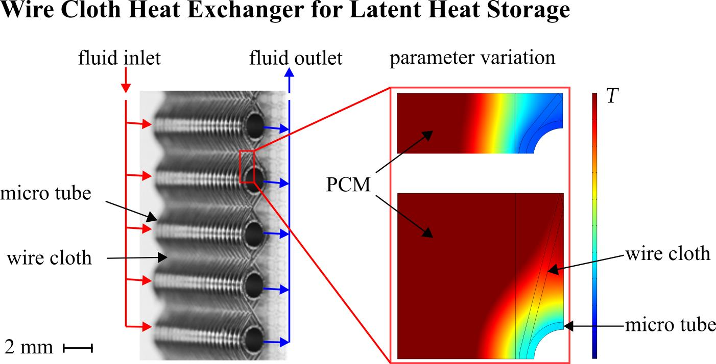
2.1. Wire Cloth Heat Exchanger

Figure 1a illustrates the wire cloth heat exchanger. The HTF flow through the tube is indicated. The PCM is located on the outside in contact with the wire cloth and tube (not shown in the figure). The complete structure is made of stainless steel, which would also allow the use of corrosive PCMs like salt hydrates. The wires are diffusion welded to the micro tubes, ensuring a good thermal contact. The small tube diameter allows to withstand high pressure, which is needed for example for high temperature storages for industrial processes including evaporation processes. Furthermore, the weaving process allows the manufacturing of large-scale heat exchanger elements, and also curved shapes are possible as the wire cloth is flexible [30]. Due to the high heat transfer area and low volume fraction of the wire, the heat exchanger can be used especially for applications with high power and storage density requirements. For the experimental set up, several wire cloth heat exchangers are arranged in parallel immersed in the PCM. Figure 1b shows a characteristic element of the wire cloth structure of two parallel heat exchangers. The geometrical parameters characterizing the heat exchanger are indicated in the figure.

For the experimental characterization, heat exchangers with a size of 250 × 250 mm² were manufactured. For this contribution, we investigated a tube pitch ($t_2$) of 5.25 mm requiring 47 micro tubes per cloth. The geometrical properties are listed in

Table 1. Properties of the investigated wire cloth heat exchangers.

Specification	Parameter	Unit	Value
number of tubes	$n_{\mathrm{tubes}}$	1	47
width of heat exchanger	$w_{\mathrm{HX}}$	mm	250
height of heat exchanger	$h_{\mathrm{HX}}$	mm	250
outer diameter tubes	$d_2$	mm	2
wall thickness tubes	$d_{\mathrm{wall}}$	mm	0.2
tube pitch perpendicular to flow direction	$t_2$	mm	5.25
wire diameter	$d_1$	µm	200
wire pitch in flow direction	$t_1$	µm	200
heat transfer surface area PCM side	$A_{\mathrm{HTS},\mathrm{PCM}}$	m2	0.2849

. The material properties for the used stainless steel are provided in Table 8 in Section 3.2. For manufacturing, heat exchanger cloths were connected to manifolds made out of 3D printed polyamide (see Figure 2).

The developed manifold design allows arranging several heat exchangers in parallel with a minimal distance $w_{\mathrm{PCM}}$ of 9 mm. The manifolds are designed to ensure a homogenous flow through all capillary tubes. Furthermore, the temperature at the inlet and outlet of each heat exchanger can be measured.

2.2. Phase Change Material

As PCM, we use the commercially available paraffin RT35HC (Rubitherm, Berlin, Germany). With a nominal melting range between 34 and 36 °C, it can be utilized for heating applications in buildings or cooling of electronic devices like batteries. The material properties are listed in

Table 2. Material properties of RT35HC.

Specification	Parameter	Unit	Value
thermal conductivity, solid state	${\lambda }_{\mathrm{PCM},\mathrm{s}}$	W/m/K	0.65
thermal conductivity, liquid state	${\lambda }_{\mathrm{PCM},\mathrm{l}}$	W/m/K	0.166
dynamic viscosity	$\eta$	Pas	0.0044
density, solid state	${\rho }_{\mathrm{PCM},\mathrm{s}}$	kg/m3	830.9
density, liquid state	${\rho }_{\mathrm{PCM},\mathrm{l}}$	kg/m3	778.2
volumetric thermal expansion coefficient	$\beta$	1/K	8.65 × 10−4
melting enthalpy	$\mathsf{\Delta }{h}_{\mathrm{m}}$	kJ/kg	222.44
melting temperature (peak)	$T_{\mathrm{m}}$	°C	36.2

and were taken from literature [32]. The melting and crystallization behavior was measured at Fraunhofer ISE by differential scanning calorimetry (DSC) according to [33]. The measurement was performed with a Discovery Q2500 DSC (TA Instruments, New Castle, Delaware, USA) in a temperature range from 10 to 45 °C. To reduce the influence of the heating rate, a heating rate test was performed. Heating rates of 8, 4, 2, 1, 0.5 and 0.25 K/min were investigated. According to [33], the peak temperature should change by less than 0.2 K when the heating rate is reduced. To fulfill these criteria, a heating rate of 0.5 K/min was selected. The sample size was 16.02 mg.

For the numerical simulations, the phase change is modeled with the apparent heat capacity. Therefore, the temperature dependent heat capacity is derived from the DSC characterization. The apparent capacity $c_{\mathrm{p}}$ is calculated as the first derivative of the enthalpy with respect to temperature $T$, i.e.,

$$c_{\mathrm{p}}=\frac{\mathrm{d}h}{\mathrm{d}T}$$

(1)

The enthalpy temperature relation is shown in Figure 3a. While for the melting, a continuous single phase change is detected for the crystallization, a second phase transition is visible at around 32 °C. As this supercooling is small in comparison to the overall phase transition from liquid to solid, it is neglected by interpolation as shown in the figure. This simplifies the modeling of the phase change transition process and allows to speed up the simulation while the storage capacity is preserved. The derived apparent heat capacity for melting and crystallization considering the interpolation is shown in Figure 3b.

The transition of thermal conductivity from solid to liquid state is modeled with a transition function indicating the state of phase $\phi$, whereby $\phi$ takes values between 0 to 1 for complete solid to complete liquid state. Commonly a smoothed step or ramp function is applied [14,34]. In this paper, we propose a transition function based on the phase change behavior determined by the DSC results. A similar approach was developed by Barz and Sommer in [35]. They used the results of different heating and cooling rates to extrapolate the behavior for a hypothetical zero heating and cooling rate. For the extrapolation, the apparent heat capacity needs to be approximated with a Weibull density function. The aim is to eliminate the rate dependency of the DSC results. In this contribution we already reduced the influence of the heating rate significantly by the heating rate test. Therefore, we directly use the DSC results. The determination of $\phi$ is based on the apparent heat capacity shown in Figure 3b. The latent part of the heat capacity is calculated by subtracting the sensible part from the total apparent heat capacity. Therefore, a linear interpolated baseline between solid and liquid state is. By integration of the latent part of the heat capacity and normalization to a maximum value of 1, the phase transition function is determined. The transition functions are shown in Figure 4.

2.3. Performance Parameter

For the performance of heat exchangers, different parameters are described in literature. Next to the mean thermal power [27], the mean effectiveness [17], combined parameter like thermal power normalized to temperature step and heat transfer surface [27] or overall heat transfer coefficient to total volume [28] are used. Similarly, Lazaro et al. describe in [36] the mean thermal power normalized to storage volume and temperature difference. There is still an ongoing discussion on the selection of performance parameters to allow a comparability of heat exchangers for latent heat storages. Especially the comparison of different operation conditions and PCMs is crucial.

In this study, the wire cloth heat exchanger to a tube bundle heat exchanger is compared for equal temperature boundary conditions. Hence, the mean thermal power is an appropriate parameter. To consider different volumes of the heat exchanger, the volume specific mean thermal power ${\overline{\dot{Q}}}_{\mathrm{v}}$ was chosen for the comparison

$${\overline{\dot{Q}}}_{\mathrm{v}}=\frac{\overline{\dot{Q}}}{V},$$

(2)

where $V$ is the storage volume and $\overline{\dot{Q}}$ is the mean thermal power. $\overline{\dot{Q}}$ is determined by an energy-based averaging proposed by Lazaro et al. [36]

$$\overline{\dot{Q}}=\frac{1}{Q_{\mathrm{end}}}{{\displaystyle \int }}_0^{Q_{\mathrm{end}}}\dot{Q}dQ.$$

(3)

By the energy-based averaging method, periods with a small energy exchange are weighted less compared to periods with high energy exchange. This is beneficial especially at the end of the phase change where the storage temperature converges to the stationary end value and a small energy amount is transferred within a long period of time. By the energy-based averaging, the results are not that sensitive to the end criterion compared to a time-averaging method. This was also concluded by Lazaro et al. [36]. $Q_{\mathrm{end}}$ is chosen as 90 percent of the total transferred energy.

It is obvious that with a high volume fraction of heat exchanger within the storage, also a high thermal power is possible, but this will lead to a reduced amount of PCM. So, it is also important to compare the storage capacity. Therefore, the volume specific storage capacity $Q_{\mathrm{v}}$ was chosen as second parameter

$$Q_{\mathrm{v}}=\frac{Q}{V},$$

(4)

where $Q$ denotes the total amount of transferred heat until the stationary temperature of the storage is reached.

For the comparison of the wire cloth exchanger and tube bundle heat exchanger, we use the ratio of the performance parameters of wire cloth to tube bundle heat exchanger with the same tube configuration. Equations (2) and (4) become:

$${\dot{Q}}_{\mathrm{v}}^{*}=\frac{\overline{{\dot{Q}}_{\mathrm{v},\mathrm{wire}}}}{\overline{{\dot{Q}}_{\mathrm{v},\mathrm{tube}}}}$$

(5)

$$Q_{\mathrm{v}}^{*}=\frac{Q_{\mathrm{v},\mathrm{wire}}}{Q_{\mathrm{v},\mathrm{tube}}}$$

(6)

2.4. Experimental Setup

2.4.1. Storage System

A lab scale prototype illustrated in Figure 5 was built. To observe the phase transition process, a transparent storage vessel (polymethylmethacrylate, PMMA) with a wall thickness of 12 mm is chosen. The inner dimensions of the vessel are 344.5 × 74 × 296 mm³. The size allows the integration of up to eight wire cloth heat exchangers. Each heat exchanger is connected to main inlet and outlet manifolds (not shown in figure) by hoses. The main manifolds are connected to the test facility (see Section 2.4.2). For a variation of the distance between the heat exchangers, spacers made of PMMA are placed between the heat exchanger manifolds (see Figure 5b). For the sizing of the container, the thermal expansion of the different components was considered. Thus, some additional volume is provided in the storage. To ensure a defined distance between the heat exchangers, they were pressed together by four compression mounts (two are marked in Figure 5a).

During the experimental characterization, the PCM temperature was measured at three different heights in the middle of the storage. The sensor positions are illustrated in Figure 5c. The PCM’s volume change, which is associated with the phase transition can be detected by an ultrasonic level sensor. To reduce heat losses/gains from the environment, the storage and the connection hoses were insulated. For the storage container, a layer of 96 mm flexible elastomeric foam was used. The individual hoses were insulated with the same foam with a thickness of 8 mm. In addition, an insulating housing made of 120 mm thick PU foam is used for all hoses and connections. The material properties of all used materials from the storage system are listed in

Table 3. Material properties of storage systems.

Parameter	Unit	PMMA [37]	Silicone [38]	Polyamide [39]	Elastomeric Foam [40]	PU Foam [41]
thermal conductivity, $\lambda$	W/m/K	0.19	0.35	0.7	0.033	0.036
density $\rho$	kg/m3	1190	1200	1000	-	-
$\mathrm{specific} \mathrm{heat} \mathrm{capacity}, {\mathrm{c}}_{\mathrm{p}}$	J/kg/K	1500	1000	1640	-	-

.

2.4.2. Test Facility

The storage system was characterized using a test facility at Fraunhofer ISE. The possible temperature range is −20 to 90 °C. The mass flow can be varied between 40 and 800 kg/h. A flow chart of the test facility is shown in Figure 6. Water ethylene glycol with a mixing ratio of 1:1 serves as HTF. The specific heat capacity was measured at Fraunhofer ISE by Q200 DSC (TA Instruments, New Castle, Delaware, USA) with an uncertainty of 5%. The temperature depended density, thermal conductivity and viscosity were taken from literature [42].

A thermostat with an integrated pump is used to control the HTF´s temperature. The control valve and the throttle valve utilized to control the mass flow rate. By means of two magnet valves, temperature steps are provided for the characterization of the storage. The mass flow is measured using a Coriolis mass flow meter (F100). The temperatures are measured with Pt100 sensors (T) at the main inlet and outlet manifold of the storage (T100, T101), at each heat exchanger inlet and outlet (not shown in the diagram), inside the storage (indicated by T103) and at the bypass (T102). Moreover, the ambient temperature is measured next to the storage (not shown in the diagram). The pressure drop of the storage can be measured with differential pressure transmitter (PD100). Further, the ultrasonic level sensor is shown (L100).

The thermal power of the storage is determined from the mass flow $\dot{m}$, the specific heat capacity $c_{\mathrm{p},\mathrm{HTF}}$ and the difference between the outlet and inlet temperature $T_{\mathrm{out},\mathrm{meas}}$ and $T_{\mathrm{in},\mathrm{meas}}$.

$${\dot{Q}}_{\mathrm{meas}}\left(t\right)=\dot{m}\left(t\right)c_{\mathrm{p},\mathrm{HTF}}\left(t\right)\left(T_{\mathrm{out},\mathrm{meas}}\left(t\right)-T_{\mathrm{in},\mathrm{meas}}\left(t\right)\right).$$

(7)

The measurement uncertainties of the sensors are given in

Table 4. Installed sensors and standard uncertainties with a rectangular distribution.

Measured Variable	Technology	Range	Standard Uncertainty
temperature	Pt100 rod sensor	−30–60 °C	0.075 K
mass flow rate	Coriolis sensor	17–680 kg/h	3.4 kg/h
pressure drop	differential pressure transmitter	0–400 mbar	0.3 mbar
PCM level change	ultrasonic level sensor	2–82 mm	0.6 mm

. Based on these, the uncertainty of the measured values and the thermal power is calculated according to Gaussian error propagation. For the evaluation and diagrams, the uncertainty is given as expanded uncertainty. Thus, 95% of the data are within the uncertainty interval.

2.4.3. Measurement Procedure

For the characterization of the heat exchanger in PCM, we investigated the performance during crystallization and melting. The following procedure is carried out: In a first step, the complete storage is heated to an initial temperature above the melting temperature of the PCM. Then, the storage is bypassed while the HTF is cooled to a temperature below the melting temperature. As soon as the HTF has reached the required temperature, it is redirect through the storage. As soon as the crystallization is finished, the same procedure is repeated but with a target temperature for the HTF, which is above the PCM´s melting temperature. Each cycle (cooling and heating to a certain temperature) is repeated three times to ensure the reproducibility of the experiment.

2.4.4. Determination of Heat Losses

Due to the unfavorable surface to volume ratio of the storage system, heat losses must be considered for the characterization although they are reduced by the insulation. The losses are determined in stationary periods of the charging and discharging procedure according to [12,43]. Figure 7 shows typical inlet and outlet temperatures of the storage over time. The times $t_1$, $t_2$ and $t_3$ mark the end of the stationary periods of each section.

The heat loss ${\dot{Q}}_{\mathrm{loss}}$ is calculated as the average thermal power of the storage for the last five minutes of the stationary period. As an extended procedure compared to [12,43], the heat loss during each phase transition period is considered introducing a transition function between the stationary periods before and after each phase change period. It is assumed that the heat losses are dependent on the mean fluid temperature between inlet and outlet of the storage $T_{\mathrm{HTF},\mathrm{mean}}$ while the ambient temperature is constant.

The following time dependent transition function $\delta \left(t\right)$ is defined for each phase transition period

$$\delta \left(t\right)=\frac{\mathsf{\Delta }{T}_{\mathrm{HTF},\mathrm{mean}}\left(t\right)}{\max \left(\mathsf{\Delta }{T}_{\mathrm{HTF},\mathrm{mean}}\left(t\right)\right) }$$

(8)

with

$$\Delta T_{\mathrm{HTF},\mathrm{mean}}\left(t\right)=\left|T_{\mathrm{HTF},\mathrm{mean}}\left(t\right)-T_{\mathrm{HTF},\mathrm{mean}}\left(t_{\mathrm{end}}\right)\right|$$

(9)

where $t_{\mathrm{end}}$ is the end time of the respective phase transition period. The thermal loss ${\dot{Q}}_{\mathrm{loss}}\left(t\right)$ is calculated by

$${\dot{Q}}_{\mathrm{loss}}\left(t\right)=\left({\dot{Q}}_{\mathrm{loss},1 }-{\dot{Q}}_{\mathrm{loss},2}\right)\delta \left(t\right)+{\dot{Q}}_{\mathrm{loss},2},$$

(10)

where subscripts 1 and 2 indicate the loss during the stationary period respectively before and after the respective phase transition.

Considering the heat loss ${\dot{Q}}_{\mathrm{loss}}$, a corrected thermal power $\dot{Q}\left(t\right)$ can be determined

$$\dot{Q}\left(t\right)={\dot{Q}}_{\mathrm{meas}}\left(t\right)-{\dot{Q}}_{\mathrm{loss}}\left(t\right).$$

(11)

With the heat loss, the inlet and outlet temperature are corrected. The temperatures are measured at the main manifolds. The heat exchangers are connected with hoses to the main manifolds. As mentioned in Section 2.4.1, a Styrodur insulation (BASF SE, Ludwigshafen, Germany) is applied for the hoses. Nevertheless, the highest losses are expected at the hoses due to the complex installation. Therefore, we assume that half of the losses occur each between the inlet temperature sensor and the storage and between the storage and the outlet temperature sensor. This assumption is proven as there is a good agreement of the corrected inlet and outlet temperature and the PCM temperatures in the storage during the stationary periods. The temperatures are corrected by

$$T_{\mathrm{in}}=\frac{{\dot{Q}}_{\mathrm{loss}}\left(t\right)}{2\dot{m}\left(t\right)c_{\mathrm{p},\mathrm{HTF}}\left(t\right)}+T_{\mathrm{in},\mathrm{meas}}\left(t\right)$$

(12)

$$T_{\mathrm{out}}=T_{\mathrm{out},\mathrm{meas}}\left(t\right)-\frac{{\dot{Q}}_{\mathrm{loss}}\left(t\right)}{2\dot{m}\left(t\right)c_{\mathrm{p},\mathrm{HTF}}\left(t\right)}$$

(13)

2.5. Model Description

For the numerical simulations, we developed a FEM model in COMSOL 5.5. To decrease the simulation time, only a characteristic section of a heat exchanger is modeled. The model considers the PCM, the wire cloth structure, a micro tube and the HTF within the tube. For the validation additional components of the storage system are considered. The applied material properties of the relevant components are listed in Table 2, Table 3 and Table 8. The geometrical parameters for the heat exchanger are given in Table 1. The following assumptions and simplification are applied:

• Volumetric expansion of the PCM during phase change is neglected.
• The PCM is treated as a solid body for both the solid and the liquid state.
• The heat transfer in PCM is based on heat conduction only.
• Natural convection is considered by an enhanced thermal conductivity method.
• Fully developed flow in the micro tubes.
• Negligible thermal gradient within the HTF perpendicular to flow direction, thus, 1D modeling is possible.
• Constant properties of HTF.
• Heat transfer between HTF and tube wall is defined by Nusselt—correlation from literature for constant wall temperature.

2.5.1. Geometry

The geometry is reduced to a symmetrical element around a single tube. As convection within the PCM is not modeled by a motion of the PCM, the reduction of the geometry to single tube is feasible. During operation, the phase change front is moving perpendicular but also parallel to the HTF flow. Therefore, it is necessary to consider the full length of the tube. Especially at low mass flow rates this effect becomes significant.

To shorten the simulation time, we decreased the complexity of the wire cloth. A characteristic element of the wire cloth heat exchanger is shown in Figure 8a. For the simplification, the 3D structure was first reduced to 2D geometry under consideration of possible symmetries (see Figure 8b). The wire cloth area considers the wire as well as the PCM by effective material properties for density $\rho$, specific heat capacity $c_{\mathrm{p}}$ and thermal conductivity $\lambda$. The properties are calculated based on the volume fraction of PCM $r_{\mathrm{PCM}}$ in the cross section according to

$${\zeta }_{\mathrm{eff}}\left(T\right)={\zeta }_{\mathrm{PCM}}\left(T\right)r_{\mathrm{PCM}}+{\zeta }_{\mathrm{wire}}\left(1-r_{\mathrm{PCM}}\right)$$

(14)

where $\zeta$ represent the respective material property. For the thermal conductivity, Equation (14) results in a parallel connection of the thermal resistances of PCM and wire. Therefore, the PCM and wire are considered as parallel rods of equal length with cross section areas according to their volume fraction.

At the contact line between wire and tube, a body is implemented to reduce the complexity of the spatial discretization as small mesh elements at the contact line are prevented. In a preliminary study with a fully discretized contact region without the contact body, it was found that by a proper sizing of the contact body, the influence on the heat transfer characteristic is negligible but the discretization effort is reduced.

The 2D structure is extruded to 3D to the full length of the tubes. The HTF is modeled as a 1D fluid flow and coupled with the 3D model on the complete length. This coupling was developed by Wittstadt [44] and adopted by Neumann et al. [14] for the modeling of a finned tube heat exchanger. The complete model is shown in Figure 9.

2.5.2. Governing Equations

The temperature distribution in the PCM and heat exchanger structure is calculated by the time-dependent temperature diffusion equation

$$\rho c_{\mathrm{p}}\frac{\partial T}{\partial t}-\nabla \left(\lambda \nabla T\right)=0$$

(15)

The temperature of the HTF is calculated by the convection–diffusion equation

$$\rho c_{\mathrm{p},\mathrm{HTF}}\left(\frac{\partial T}{\partial t}+u\nabla T\right)-\nabla \left(\lambda \nabla T\right)=0$$

(16)

where $u$ is the velocity of the HTF.

2.5.3. Boundary Conditions Validation Model

All boundary conditions are summarized in

Table 5. Overview of boundary conditions.

Boundary	Condition
$T_{\mathrm{add},k}$$\mathrm{to} T_{\mathrm{HTF}}$	convection according to Equation (18)
$T_{\mathrm{add},\mathrm{cont}}$$\mathrm{to} T_{Y_1}$	conduction according to Equation (19)
$T_{\mathrm{tube},\mathrm{inside}}$$\mathrm{to} T_{\mathrm{HTF}}$	convection according to Equation (17)
Additional PCM of experiment	considered as discretized volume
Outer surfaces	$\frac{\partial T}{\partial \overrightarrow{n}}=0$
Inlet of HTF	$T=T_{\mathrm{in}}$
Outlet of HTF	$\frac{\partial T}{\partial x}=0$

. The HTF and micro tube are coupled on the inner side of the tube by a convection coefficient

$$\dot{q}\left(x\right)=\alpha \left(T_{\mathrm{HTF}}\left(x\right)-\overline{T_{\mathrm{tube},\mathrm{inside}}} \left(x\right)\right)$$

(17)

The local heat flux density $\dot{q}$ depends on the convection coefficient $\alpha$, the local HTF temperature $T_{\mathrm{HTF}}\left(x\right)$ and the local mean perimeter temperature $\overline{T_{\mathrm{tube},\mathrm{inside}}} \left(x\right)$ of inner tube wall. The heat transfer coefficient is calculated by Nusselt correlation according to VDI Heat Atlas [45] for a pipe flow.

For validation purposes, the 1D domain HTF model is extended at the inlet and outlet by the length of the connection hoses and main manifolds. Thereby, the complete HTF volume of the measurement and additional capacities of auxiliary components $C_{\mathrm{add}}$ are considered. For every additional capacity, a single temperature node is implemented and coupled with the according HTF section. Figure 10 shows the model in top view with the extensions.

The heat transfer between the additional capacities and the HTF is determined by

$$C_{\mathrm{add},k}\frac{\partial T_{\mathrm{add},k}}{\partial t}={{\displaystyle \int }}_{x_{k,1}}^{x_{k,2}}{\alpha }_k{U}_{inside,k}\left(T_{\mathrm{add},k}-T_{\mathrm{HTF}}\left(x\right)\right) \mathrm{d}x$$

(18)

where k indicates the individual capacity. The main manifolds, silicone hoses, 3D-printed manifolds and the spacers between the heat exchanger manifolds before and after the micro tubes are considered. The latter three are combined in on capacity for inlet and outlet. Furthermore, the capacity of the container is considered similarly on the symmetry surface Y₁ of the PCM by

$$C_{\mathrm{add},\mathrm{cont}}\frac{\partial T_{\mathrm{add},\mathrm{cont}}}{\partial t}=\underset{Y_1}{\overset{}{{\displaystyle \iint }}}\frac{2{\lambda }_{\mathrm{cont}}}{t_{\mathrm{cont}}}\left(T\left(x,z\right)-T_{\mathrm{add},\mathrm{cont}}\right)\mathrm{d}\sigma .$$

(19)

As the container wall is not discretized in 3D, a thermal resistance between the wall and the capacity needs to be defined. For simplification, the thermal resistance is defined by the thermal conductivity and the half thickness of the container wall. Since only a quarter of a pipe is considered in the 3D domain, only the corresponding share of the respective additional capacity of the complete storage is taken into account.

At last, the extra PCM mass of the measurement caused by manufacturing tolerances needs to be considered. Therefore, the nominal width of the PCM $w_{\mathrm{PCM}}$ is extended by an additional thickness of PCM. The thickness is calculated based on the difference between the mass of PCM for the measurement and the nominal mass for the simulation model. For the validation experiments (see Section 3.1), we used 4.3 kg PCM, while for the according model, the nominal mass is 3.6 kg.

For symmetry reasons, a Neumann boundary condition is applied on all other outer surfaces of the PCM and heat exchanger structure. At the inlet of the HTF, a Dirichlet boundary condition is applied and, at the outlet, a Neumann condition.

2.5.4. Simplification for Performance Evaluation Model

The model will be used for a general performance evaluation of the wire cloth compared to tube heat exchanger. For a reduced computational effort, we utilized only a 2D model of the cross section of the PCM and the heat exchanger like it is shown in Figure 8b. The HTF is not modeled explicitly. The following simplifications are made:

• Neglection of heat transfer in $x$-direction;
• Constant HTF temperature;
• Neglection of heat losses;
• Neglection of auxiliary components like storage container and connection hoses.

The HTF in the tube is modeled as a single temperature node and coupled with the inner tube wall via a heat transfer coefficient according to Equation (17). By the reduction to a 2D model, the movement of the phase change front perpendicular to the 2D model is neglected.

2.5.5. Modeling of Phase Change

The phase change enthalpy of the PCM is considered by the apparent heat capacity method. The change of the thermal conductivity is considered by the derived phase transition function $\phi$ (see Section 2.2)

$$\lambda \left(T\right)=\left({\lambda }_{\mathrm{PCM},\mathrm{l}}-{\lambda }_{\mathrm{PCM},\mathrm{s}}\right)\phi \left(T\right)+{\lambda }_{\mathrm{PCM},\mathrm{s}}.$$

(20)

The density change during phase transition leads to an expansion during melting. Due to fixed volume of the simulation domain, it is necessary to set the PCM density as constant to the higher value of the solid state. Otherwise, there would be a lack of PCM mass resulting in loss of storage capacity.

Heat transfer by convection is implemented by an effective thermal conductivity [46]. During melting, the conductivity of the liquid PCM is enhanced in dependence of the width of the melted volume fraction. It is assumed that convection will arise only in region PCM₁ (see Figure 8b). In region PCM₂, convection is neglected. Due to the small width and height of the region, the occurrence of natural convection is highly limited. This is shown for example in [47]. Moreover, the region PCM₁ is assumed to be rectangular. This is feasible as the region represents the almost rectangular gap between two heat exchangers. The effective thermal conductivity ${\lambda }_{\mathrm{eff}}$ for the liquid PCM is calculated at every time step by

$${\lambda }_{\mathrm{eff}}={\lambda }_{\mathrm{PCM},\mathrm{l}}a{\mathrm{Ra}}^b.$$

(21)

The constants $a=0.1$ and b $=0.25$ are empirical determined by [46] for a rectangular PCM cavity heated from one side. The effective thermal conductivity is limited downwards by the PCM´s liquid thermal conductivity. The Rayleigh number $\mathrm{Ra}$ indicates the effect of natural convection and is estimated by

$$\mathrm{Ra}=\frac{g\beta {\rho }_{\mathrm{PCM},\mathrm{l}}^2{c}_{\mathrm{p},\mathrm{PCM},\mathrm{l}}\left(\overline{T_{\mathrm{wire}}}-T_{\mathrm{PCM}}\right)w^3}{{\eta }_{\mathrm{PCM}}{\lambda }_{\mathrm{PCM},\mathrm{l}}}.$$

(22)

Equation (22) contains the width $w$ of the melted PCM, the mean wire cloth temperature $\overline{T_{\mathrm{wire}}},$ the PCM temperature $T_{\mathrm{PCM}}$ and the gravitational acceleration $g=9.81 m/s^2$. $\overline{T_{\mathrm{wire}}}$ is calculated as the mean of the wire cloth region in Figure 8b. $T_{\mathrm{PCM}}$ denotes the mean temperature of the PCM at the edge for $y=w_{\mathrm{pcm}}/2$ on the surfaces X₁ to X₅. The width of the melted PCM $w$ is calculated on the surfaces X₁ to X₅ in region PCM₁. In x-direction between the surfaces, the value of $T_{\mathrm{PCM}}$ and $w$ are linear interpolated. The width $w$ is calculated as the mean width of the melted PCM by

$$w=\frac{2}{t_2}\underset{{\mathrm{PCM}}_1}{\overset{}{{\displaystyle \iint }}}fd\sigma$$

(23)

where $f$ indicates the discrete state of phase. It is defined by

$$f≔\left\{\begin{array}{ll}0:& \phi <0.5\\ 1:& \phi \ge 0.5\end{array}\right.$$

(24)

With this definition, the PCM is assumed to be melted if $\phi$ reaches a value of 0.5.

An interpolation for $w$ is applied as the evaluation of the integral in Equation (23) on the full PCM domain leads to extensive calculation effort.

2.5.6. Discretization

The spatial discretization for the 3D domain is based on a combination of triangle and quad mesh elements defined on surface S1 in dependence of the wire diameter. The surface mesh is extruded to the full domain with constant element length in $x$-direction. Since the main propagation direction of the phase change front is expected to be perpendicular to the $x$-direction, the element length is selected considerably larger than for the surface mesh. The 1D HTF domain is discretized by elements of equal length. We performed a discretization study to identify a proper spatial and time discretization. The study was carried out for a geometry with a tube pitch $t_2$ of 5.25 mm, a wire diameter $d_1$ of 0.2 mm and a tube diameter of $d_2$ of 2 mm. For a reduced time effort, a small distance between the heat exchangers $w_{\mathrm{PCM}}$ of 2.8 mm was applied. Four different configurations for the mesh with varying size of the elements for the surface mesh and the length of the elements in the $x$-direction were examined. The maximum allowed time step $\mathsf{\Delta }{t}_{\max }$ was varied between 1 and 60 s. The finest and coarsest mesh are shown exemplary in Figure 11.

The mass flow per heat exchanger with 47 tubes was set to the maximum applied mass flow for the measurement (see Section 3.1) of 88.5 kg/h and a temperature step at the inlet $\mathsf{\Delta }{T}_{\mathrm{step}}$ of 20 K.

The influence of the discretization is investigated for the mean volume specific power ${\overline{\dot{Q}}}_{\mathrm{v}}$ and the outlet temperature of the HTF $T_{\mathrm{out}}$. The relative deviation $\mathsf{\Delta }{\overline{\dot{Q}}}_{\mathrm{v},\mathrm{rel}}$ of ${\overline{\dot{Q}}}_{\mathrm{v}}$ to the results of the finest spatial and time discretization is shown versus the total number of degrees of freedom $n_{\mathrm{dof}}$ in Figure 12a. As all relative deviations are below 4%, every mesh configuration is acceptable. The slight increase of $\mathsf{\Delta }{\overline{\dot{Q}}}_{\mathrm{v},\mathrm{rel}}$ for $\mathsf{\Delta }{t}_{\max }$ bigger than 1 s and the highest $n_{\mathrm{dof}}$ value of 383,051 is related to the unequal variation of the elements size on the surface mesh and the element length along $x$-direction. $T_{\mathrm{out}}$ is shown versus time for the different discretization variations in Figure 12b. The results for $\mathsf{\Delta }{t}_{\max }$ of 1 and 5 s as well as 20 and 60 s are superimposed, whereby the crystallization process takes longer for 1 and 5 s. Interestingly, the influence of $n_{\mathrm{dof}}$ becomes not visible in Figure 12b. According to these results, a maximum allowed time step of 5 s and the coarsest mesh settings resulting in $n_{\mathrm{dof}}$ of 21,857 is selected as the final discretization. The computations have been carried out on an Intel® Xeon® Gold 6136 CPU @ 3.00 GHz (Intel Corporation, Santa Clara, CA, USA) computer with 192 GB RAM using 8 cores. The selected discretization results in a computation time of 5.4 min, while the finest discretization with a maximum time step of 1 s and $n_{\mathrm{dof}}$ of 383,051 requires 262.8 min. This corresponds to a reduction by a factor of 48.6.

3. Results and Discussion

3.1. Model Validation

The model is validated using the experimental data of crystallization and melting of the storage system with two heat exchangers. The validation is done for complete mass flow rates for both heat exchanger between 40 and 177 kg/h for a temperature step of 20 K. The experimental and simulated outlet temperatures are depicted in Figure 13.

For crystallization there is a high qualitative agreement between simulation and experiment. The temperatures follow the step at the inlet from 45 to 25 °C. With a higher mass flow, a lower outlet temperature can be observed. The initial temperature drop indicates the HTF exchange on the inside of the heat exchanger as well as sensible cooling of the PCM to the melting temperature. The phase change of the material takes place between around 25 and 200 min, due to the visible temperature plateau followed by sensible cooling of the solid PCM to the final temperature of 25 °C.

The deviation to the experimental data increases with lower mass flow rates due to the uncertainty of the mass flow rate sensor. To investigate the influence of the uncertainty of the mass flow rate on the outlet temperature, we performed the simulation with a mass flow rate of 43.4 kg/h considering the uncertainty of the mass flow rate sensor (see Table 4). The results are compared with the simulation results for 40 kg/h as well as the experimental data in Figure 14. For the higher mass flow, the outlet temperature is in better agreement with the experimental data. Consequently, the uncertainty of the mass flow rate measurement causes a significant part of the deviation between model and measurement.

For the melting process, there is also a good qualitative agreement between simulation and experiment (see Figure 13b). Again, the agreement is better for high mass flow rates. First the HTF exchange and the sensible heating of the PCM take place. Between around 25 and 250 min the phase change is indicated by the plateau of the temperature. After the phase transition, the temperature increases to the final temperature of 45 °C according to the sensible heating of the liquid PCM. At the end of the phase transition, higher deviations occur. In addition to the uncertainty of the mass flow measurement, the simplified model for natural convection causes the high deviation. The enhancement of the thermal conductivity is based on the thickness of the liquid PCM. It is known that the phase change front initially moves parallel to the heat exchanger. With progressing time, the movement gets faster at higher positions and, thus, two dimensional [34,46,47]. As in the presented model only one pipe of the heat exchanger is considered, the phase change front moves in parallel to the heat exchanger. Hence, the convection in the model is too low for pipes in higher regions. This is also concluded by the experiments and simulations of Farid and Husian [46]. To consider this effect in the model the enhancement of the thermal conductivity needs to be adjusted according to the height of the pipes of the heat exchanger. To the authors’ knowledge, there is no validated functional relationship for this behavior. Nevertheless, the influence can be investigated by an assumed additional enhancement factor ${\epsilon }^{*}$ for the thermal conductivity in liquid state:

$${\lambda }_{\mathrm{eff}}\left(z\right)={\epsilon }^{*}\left(z\right){\lambda }_{\mathrm{PCM},\mathrm{l}}C{\mathrm{Ra}}^n.$$

(25)

${\epsilon }^{*}$ is dependent on the vertical position $z$. For the investigation, a linear relationship is assumed with ${\epsilon }^{*}$ equal to 1 for the lowest tube and a maximum value for the highest tube. For the investigation, the maximum value ${\epsilon }_{\max }^{*}$ is varied. Instead of performing simulations for all tubes of the heat exchanger, the outlet temperature of the storage is calculated by a linear interpolation between the results for ${\epsilon }^{*}$ equal to 1 and the results for ${\epsilon }_{\max }^{*}$. For each pipe, an equal mass flow is assumed. The overall outlet temperature is calculated as the mean of all pipes. The outlet temperature of the experiment and the simulations without and with assumed additional maximum enhancement ${\epsilon }_{\max }^{*}$ of 1.5 and 2 are shown in Figure 15 for mass flow rates of 180.4 kg/h and 43.0 kg/h, respectively. With the interpolated values of the additional enhancement, the outlet temperature is in much better agreement with the experimental result. The phase transition is finished earlier compared to results without the additional enhancement. This supports the statement that the greatest uncertainty is caused by the simplified model for natural convection. For the mass flow of 43.0 kg/h still a higher deviation is visible. Compared to measurement, especially a lower outlet temperature is reached during the melting until around 150 min. One reason could be the time-dependent increase of convection. As already mentioned, the phase transition front moves parallel to the heat exchanger at the beginning. With time, the convection increases especially in higher regions. In the simplified model the additional enhancement of the convection by ${\epsilon }^{*}$ is applied from the beginning. Thus, a higher power is achieved and the outlet temperature is reduced. For ${\epsilon }_{\max }^{*}$ of 2, additional temperature steps occur at around 120 and 150 min for mass flow of 180.4 and 43.0 kg/h. The steps are related to the linear interpolation of the outlet temperature. Due to the high additional enhancement factor, the phase transition is already finished in the upper part while it is not completed for lower part. As a result, the temperature increase at the end of the phase transition in the upper part dominates the mean outlet temperature.

A quantitative analysis of the deviation between measurement and simulation is done by the mean absolute bias error $\mathrm{MABE}$ and the root mean square error $\mathrm{RMSE}$ for the outlet temperature of the storage.

$$\mathrm{MABE}=\frac{1}{n}{\displaystyle \sum }_{j=1}^n\left|T_{\exp }\left(t_j\right)-T_{\mathrm{sim}}\left(t_j\right)\right|$$

(26)

$$\mathrm{RMSE}=\sqrt{\frac{1}{n}{\displaystyle \sum }_{j=1}^n{\left(T_{\exp }\left(t_j\right)-T_{\mathrm{sim}}\left(t_j\right)\right)}^2}$$

(27)

where $n$ is the complete number of measurement time steps.

The results for $\mathrm{MABE}$ and $\mathrm{RMSE}$ are given in

Table 6. $\mathrm{MABE}$ and $\mathrm{RMSE}$ results for all validation scenarios.

$\dot{\mathit{m}}$/kg/h	Crystallization		Melting
	$\mathbf{MABE}/\mathbf{K}$	$\mathbf{RMSE}/\mathbf{K}$	$\mathbf{MABE}/\mathbf{K}$	$\mathbf{RMSE}/\mathbf{K}$
40	0.21	0.39	0.30	0.48
59	0.09	0.17	0.16	0.29
98	0.04	0.14	0.10	0.20
177	0.02	0.09	0.06	0.13

for the data shown in Figure 13. Both the $\mathrm{MABE}$ and $\mathrm{RMSE}$ are quite low indicating the good agreement between simulation and experiment. The RMSE is higher as higher deviations are weighted more. The better agreement for crystallization is shown by lower values for $\mathrm{MABE}$ and RMSE of up to 0.09 K and 0.12 K compared to melting.

A further quantitative analysis of the deviation is done by the mean volumetric thermal power ${\overline{\dot{Q}}}_{\mathrm{v}}$. For melting and crystallization, the relative deviation between simulation and experiment $\mathsf{\Delta }{\overline{\dot{Q}}}_{\mathrm{v},\mathrm{rel}}$ is shown in Figure 16. For crystallization, the deviation ranges between 17.6 and −1.6%. When the mass flow is increased by the measurement uncertainty, the maximum deviation will decrease to 11.7% while the smallest value increases to 2.86%. For melting, deviations between 10.1 and 5.4% are reached. With an increased mass flow, a reduction to 6.7 and 2.0% is possible.

The deviations are considered as acceptable small. Due to this fact, we assume the ability of the model to describe the dominant effects to be proofed. The model is validated and can be used to evaluate the performance ability of the wire cloth structure for latent thermal energy storages.

3.2. Performance Evaluation

We evaluated the performance of the wire cloth heat exchanger in comparison to a tube bundle heat exchanger without wire cloth. In doing so, a parametric study with geometrical variation of the wire cloth and tube arrangement was performed for both types of heat exchanger. For a reduced computational effort, the 2D model without the HTF modeling was used as described in Section 2.5.4. For the calculation of the volume specific performance parameters (see Section 2.3), the storage volume is calculated by the size of the 2D model.

$$V=\frac{w_{\mathrm{pcm}}}{2} \frac{t_2}{2}{d}_1$$

(28)

The outer tube diameter $d_2$, the wire diameter $d_1$, the tube distance $t_2$ and the distance between two heat exchangers $w_{\mathrm{PCM}}$ were varied. The variations of the parameters are listed in

Table 7. Variations of the geometrical parameters.

Parameter	Unit	Min	Max	$\mathbf{\Delta }$
$d_2$	mm	0.5	5	1.125
$d_1$	mm	0.025	1	0.24375
$t_2$	mm	0.75	15	3.5625
$w_{\mathrm{pcm}}$	mm	0.75	15	3.5625

. For each parameter, five variations with an equal difference $\mathsf{\Delta }$ are considered. The variations were defined in accordance to typical wire cloth configurations [31].

Additionally to the geometrical variations, two materials for the heat exchanger were investigated. As material, stainless steel 1.4301 (see prototypes in Section 2.1) and aluminum 99.5 are investigated. The material properties are listed in

Table 8. Properties of the investigated materials.

Parameter	Unit	Stainless Steel [48]	Aluminum [49]
$\lambda$	W/m/K	15	215
$c_{\mathrm{p}}$	J/kg/K	500	900
$\rho$	kg/m3	7900	2700

.

Not all parameter combinations are geometrically possible. For example, a tube diameter of 5 mm is not possible in combination with a tube distance of 0.75 mm. So, in total 654 variants were considered for the wire cloth heat exchanger. Additionally, the reference tube bundle heat exchangers without wires but equal tube configurations were simulated.

The evaluation was made only for the crystallization of the PCM. Only a minor difference between the tube bundle and wire cloth heat exchanger by convection is expected as the tube and PCM arrangement is almost equal for both. Furthermore, the computational effort is less for the crystallization model. The initial temperature was set to 45 °C, so the storage was fully charged. Then a temperature step to 25 °C was performed to discharge the storage. A constant HTF mass flow of 1 kg/s per m³ of storage volume was assumed for all variations. At this mass flow, a laminar flow field results in the tubes for all configurations. Alternatively, a constant heat transfer coefficient or constant wall temperature can be chosen as boundary conditions at the tube wall. These are withdrawn as the comparability of the different heat exchanger configurations would not be given. A constant heat transfer coefficient would limit the performance of configurations with smaller tubes due to the smaller heat transfer surface area. A constant wall temperature is also not reasonable as the heat transfer between the HTF and the tube wall influences the overall heat transfer and, thus, the time-dependent performance.

In the following section, the thermal power and storage capacity of the wire cloth heat exchanger are first discussed. Afterwards, a comparison to the tube bundle heat exchanger is made.

3.2.1. Wire Cloth Heat Exchanger

The wire cloth performance is investigated in detail for stainless steel as material. The identified relationships are also valid for aluminum as material. The mean thermal power per volume ${\overline{\dot{Q}}}_{\mathrm{v}}$ is plotted versus the volume specific storage capacity $Q_{\mathrm{v}}$ in Figure 17. In general, a high power implies a reduced storage capacity. The higher power is reached by a higher number of pipes and wires in the storage. This results in a reduced volume available for the PCM and therefore reduces the available capacity. The highest power is reached for small values of tube diameter $d_2$, wire diameter $d_1$, tube distance $t_2$ and distance between two heat exchangers $w_{\mathrm{PCM}}$. Such combination leads to a high heat transfer surface area in relation to the storage volume. Hence, the thermal resistances are small and the power is high. Moreover, the highest storage capacities are reached for small $d_2$ and $d_1$ and high $t_2$ and $w_{\mathrm{PCM}}$ since the highest PCM fraction can be achieved due to the small heat exchanger material amount.

Due to the high number of variations, Figure 18 displays sensitivity plots to identify the relationship between the volume specific power and the individual geometry parameters. As x-axis the normalized variation of each geometry parameter ${\tau }^{*}$ is used, i.e.,

$${\tau }^{*}=\frac{{\tau }_i}{{\tau }_{\mathrm{c}}}$$

(29)

where $\tau$ is either $d_1$, $d_2$, $t_2$ or $w_{\mathrm{PCM}}$ and ${\tau }_{\mathrm{c}}$ is the central variation of each parameter resulting from Table 7. The index $i$ represents the variation number which is kept constant for all the parameters except the varied. For example, a variation of $d_1$ with $i=5$ means $d_2=5 mm$, $t_2=15 mm$ and $w_{\mathrm{PCM}}=15 mm$. For $i=2$ values of $d_2=1.625 mm$, $t_2=4.3125 mm$ and $w_{\mathrm{PCM}}=4.3125 mm$ are used. Other combinations can be identified from Table 7.

A bigger tube diameter $d_2$ and wire diameter $d_1$ increase the thermal power. The mean distance between the PCM and the heat exchanger is reduced, thus, the thermal resistance is small and the power is high. The power is more influenced by $d_2$ and $d_1$ for smaller $t_2$ and $w_{\mathrm{PCM}}$ (smaller $i$). For these cases the thickness of the PCM is smaller and the wire can significantly reduce the thermal resistance. For bigger $t_2$ and $w_{\mathrm{PCM}}$ (higher $i$) the thermal resistance is dominated by the PCM thickness between the tubes and the neighboring heat exchangers. For the tube distance $t_2$ and the distance between two heat exchangers $w_{\mathrm{PCM}}$, a smaller value increases the thermal power as the thermal resistances get reduced. A reduction of $w_{\mathrm{PCM}}$ keeps the heat exchanger geometry unchanged but reduces the thickness of the PCM by using more parallel heat exchangers. By a reduction of $t_2$, the tubes are becoming closer and more tubes are used per heat exchanger. Thus, the thickness of the PCM between the tubes is reduced. Furthermore, it should be noted that with smaller $t_2$ the heat exchanger becomes more like a plate heat exchanger and the direction of the heat flow becomes more perpendicular to the heat exchanger. Therefore, the thermal resistance between PCM and HTF decreases. Further, an increase of $t_2$ leads to a lower reduction of the power compared to an increase of $w_{\mathrm{PCM}}$. This comparison is possible because the values of the two parameters are varied equally. Due to the wire cloth, the thermal resistance between the tubes is lower compared to between the heat exchangers. This allows the thermal power to be maintained at a higher level.

3.2.2. Comparison Wire Cloth and Tube Bundle Heat Exchanger

The wire cloth exchanger is compared to bare tube bundle by evaluating the ratios of the performance parameters of wire cloth to the ones of the tube bundle heat exchangers. The ratio of the mean volume specific power is shown Figure 19 for stainless steel as material in dependence of $d_1$, $d_2$ and $w_{\mathrm{PCM}}$. Generally, the thermal power can be enhanced by the wire cloth up to a factor of 2.92. The storage capacity is reduced to a minimum factor of 0.88 as the wire cloth displaces PCM volume. The increase of thermal power is clearly dependent on the geometry parameter. With larger $d_1$, the cross section of the wire is increased and the thermal resistance gets reduced, which enhances the heat transfer. At the same time, however, the capacity is reduced more by a larger wire cloth volume. For smaller $d_2$ the wire cloth is more beneficial for the thermal power as well as for the storage capacity. Furthermore, the highest increase of thermal power is reached for smaller $w_{\mathrm{PCM}}$. The main heat transfer path shifts from $y$-direction perpendicular to the heat exchanger plane (see Figure 8b) more to $z$-direction, where the wire cloth enhances the heat transfer. With higher $w_{\mathrm{PCM}}$, the capacity is increased as the main capacity is provided by the PCM located between two heat exchangers.

In Figure 20, the same data is shown but in dependency of $t_2$ instead of $w_{\mathrm{PCM}}$. With larger tube distance $t_2$, the enhancement of thermal power is higher since the wire cloth is stretched over a larger PCM volume. Thus, the higher thermal conductivity of the wire compared to the PCM can act more advantageous. The highest increase of 2.92 for the thermal power is achieved for the largest $t_2$ of 15 mm. No clear dependency of the capacity is found for $t_2$.

The results for heat exchanger made out of aluminum are shown in Figure 21 in dependence of $d_1$, $d_2$ and $t_2$. Due to the higher thermal conductivity of aluminum of 215 versus 15 W/m/K for stainless steel, the thermal power can be increased to a maximum factor of 4.20 compared to the tube bundle. This corresponds to an increase by a factor of 1.44 compared to stainless steel. Unlike for stainless steel, the second highest increase of thermal power by the wire cloth is reached for the smallest $d_1$ of 25 µm, although the influence of $t_2$ is significantly higher for this configuration. This indicates a significant better compensation of the smaller wire cross sections by the higher conductivity of aluminum.

Contrary to the power increase, the storage capacity is reduced by the aluminum wire cloth by a factor of up to 0.85 compared to the tube bundle because of the lower density of aluminum (see Table 8). This is a further reduction of factor 0.97 compared to stainless steel.

For equal geometrical configurations, wire cloth heat exchangers offer substantially higher thermal power but slightly reduced capacity compared of tube bundle heat exchangers. For an application, the power and capacity are maybe more important than the geometrical configuration. Hence, it is necessary to investigate whether any configuration of tube heat exchanger is able to provide similar performance like the wire cloth heat exchanger. Therefore, we investigated the Pareto-optimal configurations for a high thermal power and high storage capacity. Figure 22 shows the Pareto frontier for different tube diameter for both types of heat exchanger for all evaluated geometrical configurations. Both types can provide similar high thermal power and storage capacity for steel as material. If aluminum is used the wire cloth heat exchanger will offer slightly higher frontiers. It must be kept in mind that there is also a lower number of variations for the tube heat exchanger on the frontiers. Thus, there might be even better configurations, which are not calculated. In general, the difference between the two heat exchanger types is small. Since the manufacturing effort for the wire cloth heat exchanger can be assumed to be considerably higher than for the tube bundle heat exchanger, the benefit of the wire cloth heat exchanger might be too small considering the cost of manufacturing.

4. Discussion

The developed models were validated by results of an experimental characterization of a storage system with two parallel arranged prototype wire cloth heat exchangers. The experiments were carried out for melting and crystallization of the PCM. As the measurement implies thermal losses to or gains from the ambient, a correction was made. For the correction a method based on the losses to the ambient during stationary periods before and after the phase change sequences was proposed and applied. The losses are assumed be dependent only on the mean fluid temperature between inlet and outlet of the storage. This assumption is an approximation for the real dependencies of the heat losses. For dynamic systems like the investigated storage, the heat loss is dependent on multiple parameters like the thermal resistance between the storage wall and the ambient, heat convection on the outer side of the insulation and the heat capacity of the insulation. Thus, it is very complex to determine the real time dependent heat loss.

The numerical models are based on a simplified 3D geometry of the wire cloth within the PCM. For the HTF, a 1D model was applied and coupled with the 3D model. For crystallization, the heat transfer within the PCM is purely based on conduction. During melting, natural convection was considered by an enhanced model for thermal conductivity. The model is in good agreement with the experiments for crystallization and melting but with lower deviations for crystallization. As main reason for higher uncertainties, the simplified model for natural convection is identified. The model neglects the enhanced convection in higher regions. Further the convection model was developed for planar surfaces. Especially at very beginning there could be a difference between a planar heat exchanger and the three-dimensional surface of the wire heat exchanger. As the outlet temperatures of model and experiment are in good agreement the influence is assumed to be negligible for the investigated geometry. Moreover, there could be an inhomogeneous flow through the tubes in the experiment. The overall outlet temperature results from a mixture of the individual flows in each pipe which reduces the power. For the simulation, the flow distribution is assumed to be homogenous; thus, a higher power is obtained. Further reasons for the deviation are the uncertainty of the material properties and a possible contact resistance between the heat exchanger surface and the PCM as stated in [14]. For the simulation a perfect contact between PCM and heat exchanger is assumed. In the experiment, there might be a resistance, which reduces the thermal power. Further, there could be a thermal resistance between the tubes and wires, like investigated in [30]. For the simulation, a perfect contact is assumed. Due to the high number of wires, it is likely that for the prototype, the wires are not connected perfectly to the tubes. For the performance evaluation, the wire cloth heat exchanger was compared to tube bundle heat exchanger. In doing so, a parametric study was carried out with the developed 2D model. Both the geometrical configuration as well as the material of the heat exchanger were varied as part of the parameter study. The highest power is reached for a small tube and wire diameter as well as small distances between the tubes and between two adjacent heat exchangers. For these configurations, the heat exchanger structure provides a high heat transfer surface area. Compared to pure tube heat exchanger with identical geometrical configuration, the wire cloth enhances the heat transfer. Contrary, the storage capacity is reduced as the wire structure displaces PCM. By using the 2D model, the HTF temperature is assumed to be constant, and the three-dimensional propagation of phase change front is neglected. This assumption is valid for high HTF mass flow rates resulting in small temperature change of the HTF or for a phase change of the HTF like evaporation and condensation. Otherwise, there will be a change of HTF temperature along the flow direction leading to reduced temperature difference and thus to a reduced thermal power. Nevertheless, the objective of this work to investigate the performance of the wire cloth heat exchanger can be reasonably achieved with the 2D model.

Furthermore, a Pareto-optimal analysis was done to compare the performance of the heat exchanger independently of their geometrical configuration. The Pareto frontiers were derived for a high power and high storage capacity of all configurations of both heat exchanger types. This allows a qualitative comparison of the heat exchanger types. The tube heat exchanger can reach similar performance like wire cloth heat exchanger but with a different arrangement of tubes. Thus, a significant benefit by the wire cloth is only given for equal tube arrangements. As the weaving process results surely in a higher manufacturing effort compared to the bare tubes, the application of wire cloth heat exchanger is especially beneficial for fixed tube arrangements. However, if the tube arrangement can be freely selected, tube bundle heat exchangers will be still preferable. For a quantitative evaluation a higher resolution Pareto frontier must be generated. This can be done by applying optimization algorithms for the definition of the geometrical configuration.

The results of this work can be used to dimension wire cloth heat exchangers for different applications by the usage of the developed 2D and 3D model. If the same PCM and process parameters are applied an initial geometry selection can be made by using the presented data with the need for time-consuming simulations. For this reasons, the results contribute to a faster design of latent thermal energy storage with a novel wire cloth heat exchanger.

As further research, the performance of the wire cloth heat exchanger made from aluminum should be investigated experimentally. Since the performance is higher with aluminum, the higher manufacturing effort is more acceptable. It would be also valuable to investigate the distance of the wires to each other, as this will affect the performance of wire cloth heat exchangers as well. Currently the wire area is simplified by defining effective material properties according to the mass fraction of PCM and wire. This is only valid if the neighboring wires are in contact with each other. If the wires are arranged with distance, the model must be adjusted also requiring a new validation, as for example convection can develop in a different way.

5. Conclusions

• In this work, we evaluated planar wire cloth heat exchanger for the application in LTES with the Paraffin RT35HC as PCM. The wire cloth structure is investigated the first time for LTES. For the investigation, we developed and validated FEM models for crystallization and melting of the PCM. For the performance evaluation wire cloth heat exchanger are compared to tube bundle heat exchanger. The main conclusion is as follows: Wire cloth heat exchangers offer a high heat transfer area, small volume fraction of the heat exchanger, high pressure stability and are applicable for corrosive PCMs if they were made from stainless steel.
• A correction method for heat losses for experimental characterization of latent thermal energy storages based on stationary periods before and after the phase change period is introduced.
• Developed models are validated for parallel arranged of heat exchangers with maximum mean RMSE for crystallization and melting of 0.39 and 0.48 K, respectively. The deviation of the mean volumetric thermal power is within a range of 11.7 and 2.0%.
• Compared to tube bundle heat exchanger of equal tube arrangement the wire cloth can increase the thermal power by a maximum factor of 4.20, whereas the storage capacity is reduced to a minimum factor of 0.85.
• Comparing the Pareto-optimal configurations for high power and high storage capacity, the wire cloth heat exchanger performs similarly to tube bundle heat exchanger for stainless steel as heat exchanger material. There are benefits for the wire cloth if aluminum is used.

References

- Mehling, H.; Cabeza, L.F. Heat and Cold Storage with PCM: An up to Date Introduction into Basics and Applications; Springer: Berlin/Heidelberg, Germany, 2008; ISBN 978-3-540-68556-2. [Google Scholar]
- Jegadheeswaran, S.; Pohekar, S.D. Performance enhancement in latent heat thermal storage system: A review. Renew. Sustain. Energy Rev. 2009, 13, 2225–2244. [Google Scholar] [CrossRef]
- Khan, Z.; Khan, Z.; Ghafoor, A. A review of performance enhancement of PCM based latent heat storage system within the context of materials, thermal stability and compatibility. Energy Convers. Manag. 2016, 115, 132–158. [Google Scholar] [CrossRef]
- Liu, M.; Saman, W.; Bruno, F. Review on storage materials and thermal performance enhancement techniques for high temperature phase change thermal storage systems. Renew. Sustain. Energy Rev. 2012, 16, 2118–2132. [Google Scholar] [CrossRef]
- Neumann, H.; Gamisch, S.; Gschwander, S. Comparison of RC-model and FEM-model for a PCM-plate storage including free convection. Appl. Therm. Eng. 2021, 196, 117232. [Google Scholar] [CrossRef]
- Saeed, R.M.; Schlegel, J.P.; Sawafta, R.; Kalra, V. Plate type heat exchanger for thermal energy storage and load shifting using phase change material. Energy Convers. Manag. 2019, 181, 120–132. [Google Scholar] [CrossRef]
- Johnson, M.; Fiss, M.; Klemm, T.; Eck, M. Test and Analysis of a Flat Plate Latent Heat Storage Design. Energy Procedia 2014, 57, 662–671. [Google Scholar] [CrossRef]
- Johnson, M. Experimental Testing of Various Heat Transfer Structures in a Flat Plate Thermal Energy Storage Unit. In AIP Conference Proceedings; AIP Publishing LLC: Huntington, NY, USA, 2016; Volume 1734, p. 050022. [Google Scholar]
- Agyenim, F.; Eames, P.; Smyth, M. A comparison of heat transfer enhancement in a medium temperature thermal energy storage heat exchanger using fins. Solar Energy 2009, 83, 1509–1520. [Google Scholar] [CrossRef]
- Gil, A.; Barreneche, C.; Moreno, P.; Solé, C.; Inés Fernández, A.; Cabeza, L.F. Thermal behaviour of d-mannitol when used as PCM: Comparison of results obtained by DSC and in a thermal energy storage unit at pilot plant scale. Appl. Energy 2013, 111, 1107–1113. [Google Scholar] [CrossRef]
- Gil, A.; Oró, E.; Castell, A.; Cabeza, L.F. Experimental analysis of the effectiveness of a high temperature thermal storage tank for solar cooling applications. Appl. Therm. Eng. 2013, 54, 521–527. [Google Scholar] [CrossRef]
- Laing, D.; Bauer, T.; Steinmann, W.-D.; Lehmann, D. Advanced High Temperature Latent Heat Storage System—Design and Test Results. In Proceedings of the 11th International Conference on Thermal Energy Storage (Effstock 2009), Stockholm, Sweden, 14–17 June 2009. [Google Scholar]
- Anish, R.; Mariappan, V.; Mastani Joybari, M. Experimental investigation on the melting and solidification behavior of erythritol in a horizontal shell and multi-finned tube latent heat storage unit. Appl. Therm. Eng. 2019, 161, 114194. [Google Scholar] [CrossRef]
- Neumann, H.; Palomba, V.; Frazzica, A.; Seiler, D.; Wittstadt, U.; Gschwander, S.; Restuccia, G. A simplified approach for modelling latent heat storages: Application and validation on two different fin-and-tubes heat exchangers. Appl. Therm. Eng. 2017, 125, 41–52. [Google Scholar] [CrossRef]
- Rahimi, M.; Ranjbar, A.A.; Ganji, D.D.; Sedighi, K.; Hosseini, M.J.; Bahrampoury, R. Analysis of geometrical and operational parameters of PCM in a fin and tube heat exchanger. Int. Commun. Heat Mass Transf. 2014, 53, 109–115. [Google Scholar] [CrossRef]
- Kabbara, M.; Groulx, D.; Joseph, A. Experimental investigations of a latent heat energy storage unit using finned tubes. Appl. Therm. Eng. 2016, 101, 601–611. [Google Scholar] [CrossRef]
- Tay, N.; Belusko, M.; Bruno, F. An effectiveness-NTU technique for characterising tube-in-tank phase change thermal energy storage systems. Appl. Energy 2012, 91, 309–319. [Google Scholar] [CrossRef]
- Tay, N.; Bruno, F.; Belusko, M. Comparison of pinned and finned tubes in a phase change thermal energy storage system using 5CFD6. Appl. Energy 2013, 104, 79–86. [Google Scholar] [CrossRef]
- Hejčík, J.; Charvát, P.; Klimeš, L.; Astrouski, I. A PCM-water heat exchanger with polymeric hollow fibres for latent heat thermal energy storage: A parametric study of discharging stage. jtam 2016, 54, 1285–1295. [Google Scholar] [CrossRef][Green Version]
- Yang, X.; Yu, J.; Xiao, T.; Hu, Z.; He, Y.-L. Design and operating evaluation of a finned shell-and-tube thermal energy storage unit filled with metal foam. Appl. Energy 2020, 261, 114385. [Google Scholar] [CrossRef]
- Wang, Z.; Wu, J.; Lei, D.; Liu, H.; Li, J.; Wu, Z. Experimental study on latent thermal energy storage system with gradient porosity copper foam for mid-temperature solar energy application. Appl. Energy 2020, 261, 114472. [Google Scholar] [CrossRef]
- Youssef, W.; Ge, Y.T.; Tassou, S.A. CFD modelling development and experimental validation of a phase change material (PCM) heat exchanger with spiral-wired tubes. Energy Convers. Manag. 2018, 157, 498–510. [Google Scholar] [CrossRef]
- Khan, Z.; Khan, Z.A. Performance Evaluation of Coupled Thermal Enhancement through Novel Wire-Wound Fins Design and Graphene Nano-Platelets in Shell-and-Tube Latent Heat Storage System. Energies 2021, 14, 3743. [Google Scholar] [CrossRef]
- Schlott, A.; Hörstmann, J.; Tittes, K.; Andersen, O.; Meinert, J. High Power Latent Heat Storages with 3D Wire Structures–Numerical Evaluation of Phase Change Behavior. Energy Procedia 2017, 135, 75–81. [Google Scholar] [CrossRef]
- Koller, M.; Walter, H.; Hameter, M. Transient Numerical Simulation of the Melting and Solidification Behavior of NaNO3 Using a Wire Matrix for Enhancing the Heat Transfer. Energies 2016, 9, 205. [Google Scholar] [CrossRef]
- Nakaso, K.; Teshima, H.; Yoshimura, A.; Nogami, S.; Hamada, Y.; Fukai, J. Extension of heat transfer area using carbon fiber cloths in latent heat thermal energy storage tanks. Chem. Eng. Process. Process Intensif. 2008, 47, 879–885. [Google Scholar] [CrossRef]
- Medrano, M.; Yilmaz, M.O.; Nogués, M.; Martorell, I.; Roca, J.; Cabeza, L.F. Experimental evaluation of commercial heat exchangers for use as PCM thermal storage systems. Appl. Energy 2009, 86, 2047–2055. [Google Scholar] [CrossRef]
- Delgado-Diaz, W.; Stamatiou, A.; Maranda, S.; Waser, R.; Worlitschek, J. Comparison of Heat Transfer Enhancement Techniques in Latent Heat Storage. Appl. Sci. 2020, 10, 5519. [Google Scholar] [CrossRef]
- Balzer, R. Wärmetauschvorrichtung für Einen Wärmeaustausch Zwischen Medien und Webstruktur. Patent DE102006022629, 15 November 2007. [Google Scholar]
- Fugmann, H.; Martens, S.; Balzer, R.; Brenner, M.; Schnabel, L.; Mehring, C. Performance Evaluation of Wire Cloth Micro Heat Exchangers. Energies 2020, 13, 715. [Google Scholar] [CrossRef]
- Martens, S. Modellierung und Numerische Berechnung der Thermofluiddynamischen Eigenschaften Gewebebasierter Wärmeübertrager. Ph.D. Thesis, Universität Stuttgart, Stuttgart, Germany, 2019. [Google Scholar]
- Rösler, F. Modellierung und Simulation der Phasenwechselvorgänge in Makroverkapselten Latenten Thermischen Speichern. Ph.D. Thesis, Universität Bayreuth, Bayreuth, Germany, 2014. [Google Scholar]
- Gschwander, S.; Haussmann, T.; Hagelstein, G.; Sole, A.; Diarce, G.; Hohenauer, W.; Lager, D.; Rathgeber, C.; Hennemann, P.; Lazaro, A.; et al. Standard to Determine the Heat Storage Capacity of PCM Using hf-DSC with Constant Heating/Cooling Rate (Dynamic Mode). TASK 42. Available online: http://task42.iea-shc.org/data/sites/1/publications/Task4224-Standard-to-determine-the-heat-storage-capacity-of-PCM-vers150326.pdf (accessed on 31 January 2015).
- Kheirabadi, A.C.; Groulx, D. The Effect of the Mushy-Zone Constant on Simulated Phase Change Heat Transfer. In Proceedings of the ICHMT International Symposium on Advances in Computational Heat Transfer, Piscataway, NJ, USA, 25–29 May 2015. [Google Scholar]
- Barz, T.; Sommer, A. Modeling hysteresis in the phase transition of industrial-grade solid/liquid PCM for thermal energy storages. Int. J. Heat Mass Transf. 2018, 127, 701–713. [Google Scholar] [CrossRef]
- Lázaro, A.; Delgado, M.; König-Haagen, A.; Höhlein, S.; Diarce, G. Technical performance assessment of phase change material components. In Proceedings of the SHC 2019 International Conference on Solar Heating and Cooling for Building and Industry, Santiago, Chile, 4–7 November 2019. [Google Scholar]
- Evonik Industries AG. Technical Data Sheet-PLEXIGLAS® GS/XT.; Evonik Industries AG: Essen, Germany, 2013. [Google Scholar]
- DIN German Institute for Standardization. DIN EN ISO 10456: Baustoffe und Bauprodukte: Wärme- und feuchtetechnische Eigenschaften; Beuth Verlag GmbH: Berlin, Germany, 2010. [Google Scholar]
- 3D Systems GmbH. Technical Data Sheet-DuraForm PA; 3D Systems GmbH: York County, SC, USA, 2008. [Google Scholar]
- Armacell Enterprise GmbH & Co. KG. Technical Data Sheet-Armaflex; Armacell Enterprise GmbH & Co. KG: Schönefeld, Germany, 2017. [Google Scholar]
- BASF SE. Technical Data Sheet-Styrodur; BASF SE: Ludwigshafen, Germany, 2019. [Google Scholar]
- Bell, I.H.; Wronski, J.; Quoilin, S.; Lemort, V. Pure and Pseudo-pure Fluid Thermophysical Property Evaluation and the Open-Source Thermophysical Property Library CoolProp. Ind. Eng. Chem. Res. 2014, 53, 2498–2508. [Google Scholar] [CrossRef]
- Zipf, V.; Willert, D.; Neuhäuser, A. Active latent heat storage with a screw heat exchanger–experimental results for heat transfer and concept for high pressure steam. In AIP Conference Proceedings 1734; SolarPACES 2015; AIP Publishing: Melville, NY, USA, 2016; p. 50044. ISBN 073541386X. [Google Scholar]
- Wittstadt, U. Experimentelle und Modellgestützte Charakterisierung von Adsorptionswärmeübertragern. Ph.D. Thesis, Technische Universität Berlin, Berlin, Germany, 2018. [Google Scholar]
- Gnielinski, V. VDI-Wärmeatlas-Teil G Wärmeübertragung bei Erzwungener Konvektion-G1 Durchströmte Rohre; Springer: Berlin/Heidelberg, Germany, 2013; ISBN 978-3-642-19980-6. [Google Scholar]
- Farid, M.M.; Husian, R.M. An electrical storage heater using the phase-change method of heat storage. Energy Convers. Manag. 1990, 30, 219–230. [Google Scholar] [CrossRef]
- Vogel, J.; Felbinger, J.; Johnson, M. Natural convection in high temperature flat plate latent heat thermal energy storage systems. Appl. Energy 2016, 184, 184–196. [Google Scholar] [CrossRef]
- Deutsche Edelstahlwerke GmbH. Technical Data Sheet-1.4301; Deutsche Edelstahlwerke GmbH: Witten, Germany, 2015. [Google Scholar]
- Hesse, W. (Ed.) Aluminium-Werkstoff-Datenblätter: Aluminium Material Data Sheets, 7th ed.; Beuth Verlag GmbH: Berlin, Germany, 2016; ISBN 3410268758. [Google Scholar]