A Fast Response Robust Deadbeat Predictive Current Control for Permanent Magnet Synchronous Motor

Abstract

Deadbeat predictive current control (DBPCC) has the characteristic of fast current response, but it is sensitive to motor parameters. Observer-based DBPCC can eliminate the steady state current tracking error when parameter mismatch exists. However, the actual current will deviate from the reference current during transient state in the case of inductance mismatch. In this paper, a fast response robust deadbeat predictive current control (FRRDBPCC) method is proposed for surface mounted permanent magnet synchronous motor (SPMSM). Firstly, the current tracking error caused by inductance mismatch during transient state is analyzed in detail. Then, an extended state observer (ESO) is proposed to estimate the lumped disturbance caused by parameter mismatch. Based on discrete time ESO, the predicted currents are used to replace the sampled currents to compensate for one-step delay caused by calculation and sampling. Furthermore, an online inductance identification algorithm and a modified prediction model are proposed. The dq-axis currents can be completely decoupled by updating the inductance in the modified prediction model online, ensuring that the current can track the reference value in two control periods. The proposed method improves robustness against parameter mismatch and guarantees dynamic response performance simultaneously. The experimental results verify the effectiveness of the proposed method.

1. Introduction

Due to the brilliant advantages of having a high efficiency, high power density, wide speed range and compact structure, permanent magnet synchronous motors (PMSM) have been widely used in industrial applications, such as electrical vehicles and high precision servo systems. Since the field-oriented control (FOC) method was invented, it has become one of the most popular control methods applied in PMSM [1]. In a traditional FOC-based PMSM control system, a multilayer nested loop structure with proportional–integral (PI) controllers separately aiming to maintain the speed and current at the desired value is applied [2]. Since the parameters of the PI controller directly determine the control performance, the design process tends to be important and time consuming. In order to further improve the control performance, some other algorithms, such as sliding mode controller [3], adaptive repetitive learning controller [4] and internal model controller [5] have been applied in PMSM control systems.

During the last decade, with the great improvements in microprocessor computing performance, predictive control has received more attention in academic circles for its faster dynamic response compared with the traditional PI controller [6,7,8,9,10,11,12,13,14,15,16]. Among the multiple predictive current control methods, deadbeat predictive current control (DBPCC) not only inherits a fast current-tracking performance, but also has a constant switching frequency, which allows DBPCC to be widely used [17]. DBPCC calculates the input voltage directly based on the prediction model, then translates it into corresponding switching configurations through space vector pulse width modulation [18]. However, its control performances are deteriorated by parameter mismatch. For example, since the stator resistance and flux linkage will change with temperature, the reference voltage calculated according to the model will deviate from the expected value and consequently cause current tracking errors. For the sake of achieving better control performance and improving the robustness of the DBPCC control system, some methods have been put forward, among which the strategy on the basis of disturbance suppression has been proved to be the most effective [19]. In [20], a discrete Luenberger observer is designed to predict the future value of stator current and estimate the disturbance caused by unmodeled dynamics and parameter variations. In [18], a stator current and disturbance observer based on sliding-mode exponential reaching law is proposed, which uses a nonlinear function to improve the anti-disturbance ability of the observer. In [21], to suppress the chattering problem of the traditional sliding mode observer, a high order sliding-mode observer is proposed to provide precise estimation of the disturbance and sequentially achieve fast dynamic response of the current. In [22], a composite sliding-mode disturbance observer based on the stator current is proposed to estimate the lumped disturbance and compensate for one-step delay. In [23], a novel power sliding mode reaching law and an improved non-homogeneous disturbance observer are proposed to guarantee the current tracking error converges to zero. In [24], a model-free predictive current control based on extended state observer is proposed in a stationary coordinate. Since the model parameters are not required in the controller, the robustness of the system is enhanced. In [25], a nonlinear disturbance observer is designed to estimate the total disturbance of the system for feedforward compensation, strengthening the anti-interference performance.

By applying the mentioned observer-based DBPCC methods, the steady state performance can be significantly improved and the current tracking error can be completely eliminated. However, in the case that the reference current has a step change, the error of inductance will lead to a sudden change of disturbance. Under these circumstances, the limited bandwidth of the observer will result in an error between the observed disturbance and the actual disturbance, resulting in the current tracking error.

In this paper, a fast response robust deadbeat predictive current control (FRRDBPCC) method is proposed. Firstly, the current tracking error caused by inductance error during transient state is developed explicitly based on the discrete mathematical model of the SPMSM. Secondly, an ESO-based DBPCC method is proposed to eliminate the steady state current tracking error. The stability of the whole current control loop is analyzed in detail in the discrete domain, considering the one step delay of the digital control system. Moreover, for the sake of improving the transient response performance of the control system, an online inductance identification algorithm which takes the influence of magnetic saturation into consideration is proposed. In addition, a modified prediction model is established to sufficiently decouple the d-axis and q-axis currents. Finally, the effectiveness of the proposed current control method is verified by simulation and experimental results.

2. Models of SPMSM and Analysis of Conventional Methods

2.1. Mathematical Model of SPMSM and Conventional Observer-Based DBPCC

The voltage state-space equations of SPMSM in synchronous rotating frame can be expressed as follows [7]:

$$\{\begin{array}{l}{u}_d=R{i}_d+L\frac{d{i}_d}{dt}-{\omega }_{e}L{i}_q\hfill \\ u_q=R{i}_q+L\frac{d{i}_q}{dt}+{\omega }_{e}L{i}_d+{\omega }_e{\psi }_f\hfill \end{array}$$

(1)

where $i_d$ and $i_q$ are the stator currents in the dq-axis, $u_d$ and $u_q$ are the stator voltages in the dq-axis, $L$ is the stator inductance, $R$ is the stator resistance, ${\psi }_f$ is the permanent magnet flux linkage, ${\omega }_e$ is the electrical angular velocity of the motor.

According to Equation (1), the state-space equations can be described as:

$$\{\begin{array}{l}\frac{d{i}_d}{dt}=-\frac{R}{L}{i}_d+{\omega }_e{i}_q+\frac{1}{L}{u}_d\hfill \\ \frac{d{i}_q}{dt}=-\frac{R}{L}{i}_q-{\omega }_e{i}_d-\frac{{\omega }_e{\psi }_f}{L}+\frac{1}{L}{u}_q\hfill \end{array}$$

(2)

Applying forward Euler discretization to Equation (2), the discrete voltage model of SPMSM can be written as [7]:

$$\{\begin{array}{l}{i}_d\left(k+1\right)=(1-T_{s}R/L)i_d\left(k\right)+T_s{\omega }_e(k)i_q\left(k\right)+T_s{u}_d\left(k\right)/L\hfill \\ i_q\left(k+1\right)=(1-T_{s}R/L)i_q\left(k\right)-T_s{\omega }_e(k)i_d\left(k\right)+T_s{u}_q\left(k\right)/L-T_s{\omega }_e(k){\psi }_f/L\hfill \end{array}$$

(3)

where $T_s$ represents the control period.

To predict the future state of the current, the discrete voltage prediction model used in the conventional deadbeat controller can be written as:

$$\{\begin{array}{l}{i}_{{}_d}^p\left(k+1\right)=(1-T_s{R}_0/L_0)i_d\left(k\right)+T_s{\omega }_e(k)i_q\left(k\right)+T_s{u}_d\left(k\right)/L_0\hfill \\ i_q^p\left(k+1\right)=(1-T_s{R}_0/L_0)i_q\left(k\right)-T_s{\omega }_e(k)i_d\left(k\right)+T_s{u}_q\left(k\right)/L_0-T_s{\omega }_e(k){\psi }_{f0}/L_0\hfill \end{array}$$

(4)

where $R_0$, $L_0$ and ${\psi }_{f0}$ are the nominal values of the motor parameters applied in the controller.

It can be seen from Equation (4) that the current prediction accuracy depends on the parameters of the prediction model [26]. In order to achieve better current tracking performance, many observer-based methods have been proposed, which can be expressed by Equation (5) [14].

$$\{\begin{array}{l}\frac{d{i}_d}{dt}=\frac{u_d}{L_0}+F_d\\ \frac{d{F}_d}{dt}={\eta }_d\\ \frac{d{i}_q}{dt}=\frac{u_q}{L_0}+F_q\\ \frac{d{F}_d}{dt}={\eta }_q\end{array}$$

(5)

where $L_0$ is the controller gain in dq-axis which equals the nominal value of inductance, $F_d$ and $F_q$ represent the lumped disturbance which can be extracted by different observers. ${\eta }_d$ and ${\eta }_q$ are the derivatives of $F_d$ and $F_q$, respectively.

2.2. Problems with Conventional Observer-Based DBPCC Methods

Applying forward Euler discretization to Equation (5), the discrete voltage model can be written as:

$$\{\begin{array}{l}(i_d\left(k+1\right)-i_d\left(k\right))/T_s=u_d\left(k\right)/L_0+F_d\left(k\right)\hfill \\ (i_q\left(k+1\right)-i_q\left(k\right))/T_s=u_q\left(k\right)/L_0+F_q\left(k\right)\hfill \end{array}$$

(6)

where $u_d(k)$ and $u_q(k)$ represent the average control voltage from $T_k$ to $T_{k+1}$ in dq-axis, $T_k$ represents the start time of the k-th control period, $F_d(k)$ and $F_q(k)$ represent the average lumped disturbance from $T_k$ to $T_{k+1}$ in dq-axis, which can be described as

$$\{\begin{array}{l}{F}_d\left(k\right)=\left(1/L-1/L_0\right)u_d\left(k\right)-\left(R{i}_d\left(k\right)-{\omega }_e(k)L{i}_q\left(k\right)\right)/L\hfill \\ F_q\left(k\right)=\left(1/L-1/L_0\right)u_q\left(k\right)-\left(R{i}_q\left(k\right)+{\omega }_e(k)L{i}_d\left(k\right)+{\omega }_e(k){\psi }_f\right)/L\hfill \end{array}$$

(7)

Then, the prediction model can be written as:

$$\{\begin{array}{l}(i_d^p\left(k+1\right)-i_d\left(k\right))/T_s=u_d\left(k\right)/L_0+{\widehat{F}}_d\left(k\right)\hfill \\ \left(i_q^p\left(k+1\right)-i_q\left(k\right)\right)/T_s=u_q\left(k\right)/L_0+{\widehat{F}}_q\left(k\right)\hfill \end{array}$$

(8)

where ${\widehat{F}}_d(k)$, ${\widehat{F}}_q(k)$ represent the estimated lumped disturbance.

It is assumed that the motor has operated in steady state before $T_k$ and the observer has converged before $T_k$, ${\widehat{F}}_d\left(k-1\right)=F_d\left(k-1\right)$, ${\widehat{F}}_q\left(k-1\right)=F_q\left(k-1\right)$ can be obtained. The speed of the motor can be considered constant during $T_s$. Since $i_q$ does not change before $T_k$, the estimated $F_q\left(k\right)$ equals to ${\widehat{F}}_q\left(k-1\right)$. Substituting ${\widehat{F}}_q\left(k-1\right)$ into Equation (8) and replacing $i_q^p(k+1)$ with $i_{qref}(k)$, $u_q(k)$ with $u_{qref}(k)$:

$$(i_{qref}\left(k\right)-i_q\left(k\right))/T_s=u_{qref}\left(k\right)/L_0+{\widehat{F}}_q\left(k-1\right)$$

(9)

In the steady state, $i_q\left(k\right)=i_q\left(k-1\right)$, $i_d\left(k\right)=i_d\left(k-1\right)$, ${\omega }_e(k)={\omega }_e(k-1)$. Substituting Equation (7) into Equation (9), it derives:

$$(i_{qref}\left(k\right)-i_q\left(k\right))/T_s=u_{qref}\left(k\right)/L_0+\left(1/L-1/L_0\right)u_q\left(k-1\right)-\left(R{i}_q\left(k\right)+{\omega }_e(k)L{i}_d\left(k\right)+{\omega }_e(k){\psi }_f\right)/L$$

(10)

The q-axis model of SPMSM can be written as:

$$(i_q\left(k+1\right)-i_q\left(k\right))/T_s=u_{qref}\left(k\right)/L-\left(R{i}_q\left(k\right)+{\omega }_e(k)L{i}_d\left(k\right)+{\omega }_e(k){\psi }_f\right)/L$$

(11)

Subtracting Equation (10) from Equation (11):

$$(i_q\left(k+1\right)-i_{qref}\left(k\right))/T_s=\left(1/L-1/L_0\right)\left[u_{qref}\left(k\right)-u_q\left(k-1\right)\right]$$

(12)

Simplifying Equation (10), it derives:

$$(i_{qref}\left(k\right)-i_q\left(k\right))/T_s=\left(u_{qref}\left(k\right)-u_q\left(k-1\right)\right)/L_0+\left[u_q\left(k-1\right)-R{i}_q\left(k\right)-{\omega }_e\left(k\right)L{i}_d\left(k\right)-{\omega }_e\left(k\right){\psi }_f\right]/L$$

(13)

In the steady state, it derives:

$$u_q\left(k-1\right)=R{i}_q\left(k\right)-{\omega }_e\left(k\right)L{i}_d\left(k\right)-{\omega }_e\left(k\right){\psi }_f$$

(14)

Substituting Equation (14) into Equation (13), it derives:

$$(i_{qref}\left(k\right)-i_q\left(k\right))/T_s=\left[u_{qref}\left(k\right)-u_q\left(k-1\right)\right]/L_0$$

(15)

Substituting Equation (15) into Equation (12), it derives:

$$i_q\left(k+1\right)-i_{qref}\left(k\right)=\left(L_0/L-1\right)\left[i_{qref}\left(k\right)-i_q\left(k\right)\right]$$

(16)

It can be seen from Equation (15) that it will lead to a sudden change in q-axis reference voltage in the case that the current loop is operating in transient state which normally results in a fast change in q-axis reference current. Then, if the nominal inductance is not equal to the real inductance, the lumped disturbance in q-axis, as can be seen in Equation (7), will have a sudden change. Due to the limited bandwidth of the observer, it takes several control cycles for the observer to converge. Therefore, the tracking error of current will occur. Equation (16) shows the relationship between the current tracking error and the inductance in transient state.

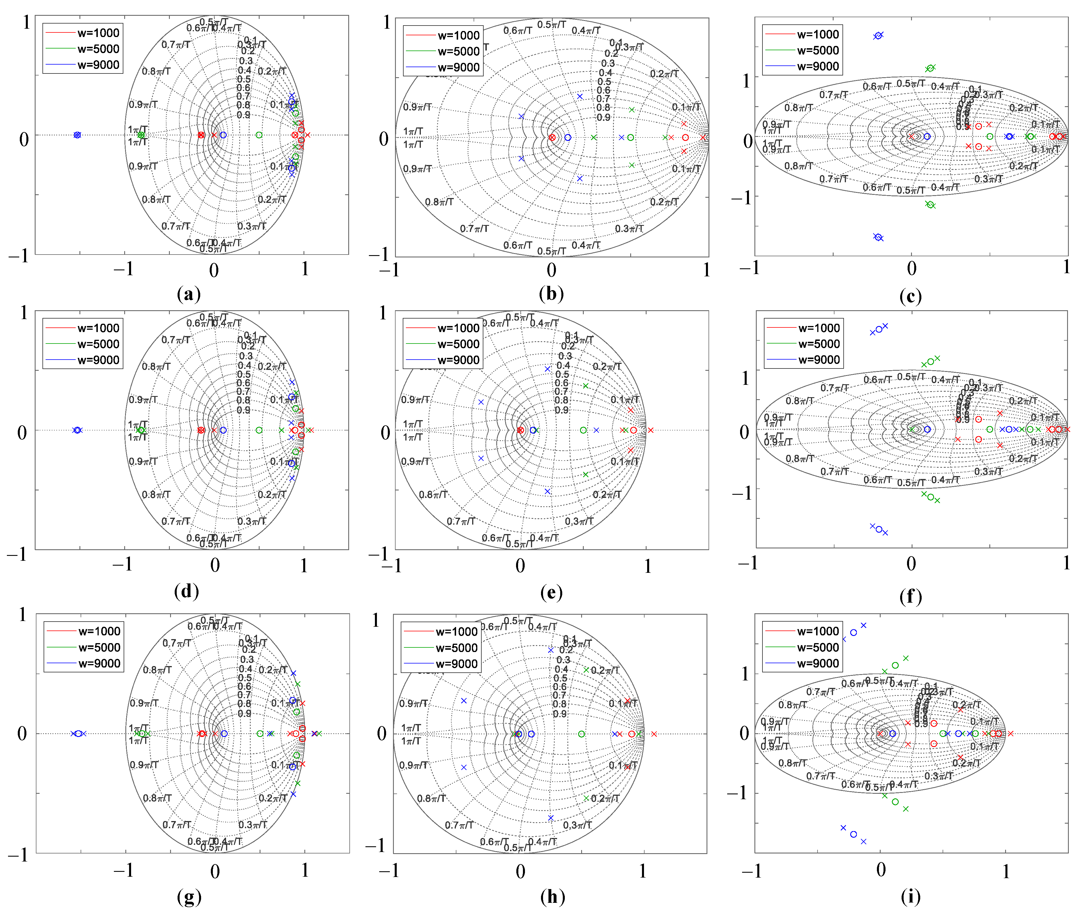
2.3. Stability Analysis of the ESO-Based DBPCC

In order to better analyze the influence of observer gain and nominal inductance on current loop control performance, a linear ESO is proposed to estimate the lumped disturbance. With this specially designed method, the lumped disturbance observer in dq-axis can be written as:

$$\{\begin{array}{l}\frac{d{\widehat{i}}_d}{dt}=\frac{u_d}{L_0}+{\widehat{F}}_d-{\beta }_1\left({\widehat{i}}_d-i_d\right)\hfill \\ \frac{d{\widehat{F}}_d}{dt}=-{\beta }_2\left({\widehat{i}}_d-i_d\right)\hfill \\ \frac{d{\widehat{i}}_q}{dt}=\frac{u_q}{L_0}+{\widehat{F}}_q-{\beta }_3\left({\widehat{i}}_q-i_q\right)\hfill \\ \frac{d{\widehat{F}}_q}{dt}=-{\beta }_4\left({\widehat{i}}_q-i_q\right)\hfill \end{array}$$

(17)

where ${\widehat{i}}_d$ and ${\widehat{i}}_q$ are the estimated stator currents in the dq-axis, ${\widehat{F}}_d$ and ${\widehat{F}}_q$ are the estimated lumped disturbance in the dq-axis, ${\beta }_1$, ${\beta }_2$, ${\beta }_3$ and ${\beta }_4$ are coefficients of the observer. Because the dq-axis equation is highly symmetric, only the d-axis equation is analyzed. Defining the estimation error in the d-axis:

$${\tilde{\mathit{I}}}_{\mathit{d}}={\left[{\tilde{i}}_d{\tilde{F}}_d\right]}^T={\left[{\widehat{i}}_d-i_d{\widehat{F}}_d-F_d\right]}^T$$

(18)

Subtracting Equation (5) from Equation (17), the d-axis error equation can be expressed as:

$$\{\begin{array}{l}{\dot{\tilde{i}}}_d={\tilde{F}}_d-{\beta }_1{\tilde{i}}_d\hfill \\ {\dot{\tilde{F}}}_d=-{\beta }_2{\tilde{i}}_d-{\eta }_d\hfill \end{array}$$

(19)

The characteristic equation of Equation (19) can be expressed as:

$$\left|sI-\left[\begin{array}{cc}-{\beta }_1& 1\\ -{\beta }_2& 0\end{array}\right]\right|=s^2+{\beta }_{1}s+{\beta }_2=0$$

(20)

In order to set the poles of Equation (20) at ${\omega }_0$, the coefficients of the ESO are chosen as ${\beta }_1=2{\omega }_0$, ${\beta }_2={\omega }_0^2$. ${\omega }_0$ represents the bandwidth of ESO. Due to the discrete nature of the digital controller, applying forward Euler discretization to Equation (19), it derives the d-axis discrete error model:

$$\{\begin{array}{l}({\widehat{i}}_d(k+1)-{\widehat{i}}_d(k))/T_s=u_d(k)/L_0+{\widehat{F}}_d(k)-{\beta }_1\left({\widehat{i}}_d(k)-i_d(k)\right)\\ ({\widehat{F}}_d(k+1)-{\widehat{F}}_d(k))/T_s=-{\beta }_2\left({\widehat{i}}_d(k)-i_d(k)\right)\end{array}$$

(21)

Applying the z-transform to Equation (21), the transfer function of ESO can be expressed as:

$$\frac{{\widehat{i}}_d(z)}{i_d(z)}=\frac{T_s{\beta }_{1}z+T_s^2{\beta }_2-T_s{\beta }_1}{z^2+({\beta }_1{T}_s-2)z+(1+{\beta }_2{T}_s{}^2-{\beta }_1{T}_s)}$$

(22)

The characteristic Equation of Equation (22) can be expressed as:

$$z^2+({\beta }_1{T}_s-2)z+(1+{\beta }_2{T}_s{}^2-{\beta }_1{T}_s)=0$$

(23)

Substituting ${\beta }_1=2{\omega }_0$, ${\beta }_2={\omega }_0^2$ into Equation (23) and solving the new equation, it derives:

$$z_{1,2}=1-{\omega }_0{T}_s$$

(24)

According to the stability theory of discrete systems, $z_{1,2}$ should be set in the unit circle. To achieve fast current response, $z_{1,2}$ should be set close to zero, which makes the value of ${\omega }_0$ larger, and the observer becomes sensitive to disturbance and easily becomes unstable. From Equations (7) and (15), when the motor is operating in transient state, the voltage changes rapidly. If the error of inductance is large, the lumped disturbance will have a high frequency variation. Then, the current tracking performance depends on whether the observer can accurately estimate the lumped disturbance without delay.

It can be inferred from the above analysis that the bandwidth of the current control loop depends not only on the gain of the observer, but also on the accuracy of the nominal inductance. Moreover, the stability of the current control loop is also affected. According to Equations (3), (8) and (17), while ignoring the influence of resistance and considering the one-step delay of the digital control system, choosing ${\beta }_1={\beta }_3=2{\omega }_0$, ${\beta }_2={\beta }_4={\omega }_0^2$, then the discrete form of the dq-axis current closed-loop response equation can be written as:

$$\{\begin{array}{l}{i}_d\left(k+1\right)-i_d\left(k\right)=T_s{\omega }_e(k)i_q\left(k\right)+T_s{u}_d\left(k-1\right)/L\hfill \\ {\widehat{i}}_d(k+1)-{\widehat{i}}_d\left(k\right)=T_s{u}_d\left(k-1\right)/L_0+T_s{\widehat{F}}_d\left(k\right)-T_s{\beta }_1\left({\widehat{i}}_d\left(k\right)-i_d\left(k\right)\right)\hfill \\ {\widehat{F}}_d(k+1)-{\widehat{F}}_d\left(k\right)=-T_s{\beta }_2\left({\widehat{i}}_d\left(k\right)-i_d\left(k\right)\right)\hfill \\ i_{dref}\left(k\right)-{\widehat{i}}_d(k+1)=T_s{u}_d\left(k\right)/L_0+T_s{\widehat{F}}_d\left(k+1\right)\hfill \\ i_q\left(k+1\right)-i_q\left(k\right)=-T_s{\omega }_e(k)i_d\left(k\right)-T_s{\omega }_e(k){\psi }_f/L+T_s{u}_q\left(k-1\right)/L\hfill \\ {\widehat{i}}_q(k+1)-{\widehat{i}}_q\left(k\right)=T_s{u}_q\left(k-1\right)/L_0+T_s{\widehat{F}}_q\left(k\right)-T_s{\beta }_1\left({\widehat{i}}_q\left(k\right)-i_q\left(k\right)\right)\hfill \\ {\widehat{F}}_q(k+1)-{\widehat{F}}_q\left(k\right)=-T_s{\beta }_2\left({\widehat{i}}_q\left(k\right)-i_q\left(k\right)\right)\hfill \\ i_{qref}\left(k\right)-{\widehat{i}}_q(k+1)=T_s{u}_q\left(k\right)/L_0+T_s{\widehat{F}}_q\left(k+1\right)\hfill \end{array}$$

(25)

Applying the z-transform to Equation (25) and considering ${\omega }_e(k){\psi }_f$ as a constant external disturbance because the time constant of the current loop is much smaller than that of the speed loop, then the transfer function of q-axis current control loop can be expressed as:

$$i_q\left(z\right)=\frac{L_0{i}_{qref}(z)((-1+z)(-1+z+T_s{\beta }_1)+T_s^2{\beta }_2)(L{(-1+z)}^{2}z+(-1+z)(L(-1+z)+L_0)T_s{\beta }_1+z{L}_0{T}_s^2{\beta }_2)}{z({(L{(-1+z)}^{2}z+(-1+z)(L(-1+z)+L_0)T_s{\beta }_1+z{L}_0{T}_s^2{\beta }_2)}^2+L^2{(-1+z)}^2{T}_s^2{(z+T_s{\beta }_1)}^2{\omega }_e^2)}$$

(26)

If the cross-coupling effect of dq-axis currents is ignored and the nominal inductance is accurate, Equation (27) can be obtained by substituting ${\omega }_e=0$ and $L_0=L$ into Equation (26).

$$i_q\left(z\right)=z^{-2}{i}_{qref}(z)$$

(27)

Two poles of Equation (27) are both located at zero which means that the current would reach to the reference value in two control periods.

Figure 1 shows the variation of closed loop zeros and poles of Equation (26) with speed, nominal inductance and observer gain. The parameter w in Figure 1 represents the selected bandwidth of the ESO. It can be seen from Figure 1a–c, when the motor is operating at ${\omega }_e=400$ (rad/s), if the inductance error is large, increasing the bandwidth of the observer will increase the chattering of the system and make it become unstable. It can be seen from Figure 1d–f that when the speed of the motor increases, the imaginary part of the poles will gradually move away from the real axis. In Figure 1g–i, if the motor is operating at ${\omega }_e=2000$ (rad/s), because the cross-coupling effect of dq-axis currents is becoming more and more serious, only when the inductance has no error and the bandwidth of the observer is relatively large can the stability of the system can be ensured. However, an excessive observer bandwidth will introduce noise and degrade the performance of the controller.

3. Proposed Methods

From the above analysis, it can be concluded that both the nominal inductance and observer gain affect the stability and control performance of the current loop. Only when the nominal inductance is chosen close to the real inductance and an appropriate gain is selected can the control performance of the current loop reach the best. Additionally, whether the current loop is fully decoupled also affects the response speed and stability of the system.

3.1. Online Inductance Identification Algorithm Considering Saturation

Considering the effect of magnetic saturation, a linear inductance model is used in this paper. Compared with the self-saturation of inductance, the cross-saturation of inductance can be neglected. Then, the inductance model for a SPMSM can be written as:

$$L_i=L_0-\alpha \ast I_i(i=d,q)$$

(28)

where $L_i$ represents the inductance in i-axis, $L_0$ represents the initial inductance without saturation, $\alpha$ represents the saturation coefficient, $I_i$ represents the current in i-axis.

For SPMSM, $i_d=0$ control is usually adopted, so the d-axis is generally not saturated. Then the identification is only carried out on the q-axis and the nominal inductance of d-axis is chosen as $L_0$. In this article, step voltages are injected into q-axis for identification. From Equation (3), neglecting the voltage drop on the resistance, the discrete voltage equation of q-axis can be written as:

$$L_q(i_q\left(k\right)-i_q\left(k-1\right))=T_s{U}_q\left(k-1\right)-T_s{\omega }_e(k-1)L_0{i}_d\left(k-1\right)-T_s{\omega }_e(k-1){\psi }_f$$

(29)

When the motor is operating in the steady state, $i_q\left(k\right)=i_q\left(k-1\right)$, ${\omega }_e(k)={\omega }_e(k-1)$. Then a step voltage signal is injected in the q-axis. Considering the magnetic saturation, it derives:

$$\overline{L}(i_q\left(k+1\right)-i_q\left(k\right))=T_s{U}_q\left(k\right)-T_s{\omega }_e(k)L_0{i}_d\left(k\right)-T_s{\omega }_e(k){\psi }_f$$

(30)

$$\overline{L}=(L_0-\alpha \ast i_q\left(k\right)+L_0-\alpha \ast i_q\left(k+1\right))/2$$

(31)

where $\overline{L}$ represents the average inductance during voltage injection. When the motor is operating at low speed, the change of ${\omega }_e{L}_0{i}_d$ can be neglected compared with the injected voltage signal. Subtracting Equation (29) from Equation (30), it derives:

$$\overline{L}(i_q\left(k+1\right)-i_q\left(k\right))/T_s=\Delta u$$

(32)

where $\Delta u$ represents the injected voltage signal. Equation (32) can be transformed into:

$$L_0-\alpha x=y$$

(33)

$$x=(i_q\left(k\right)+i_q\left(k+1\right))/2$$

(34)

$$y=\Delta u{T}_s/(i_q\left(k+1\right)-i_q\left(k\right))$$

(35)

After multiple times of voltage injection, the least square method is used to estimate $L_0$ and $\alpha$. Minimizing the following formula:

$$\underset{i=1}{\stackrel{n}{\mathsf{\Sigma }}}{\left(y_i-{\widehat{L}}_0+\widehat{\alpha }{x}_i\right)}^2$$

(36)

where $n$ represents the total number of the injected voltages. $x_i$, $y_i$ represent the value of $x$, $y$ after the i-th injection, i represents the voltage injection times at present (i = 1, 2, …, n). ${\widehat{L}}_0$, $\widehat{\alpha }$ represent the estimated value of $L_0$, $\alpha$. Then it derives:

$${\widehat{L}}_0=(\underset{i=1}{\stackrel{n}{\mathsf{\Sigma }}}{x}_i^2\underset{i=1}{\stackrel{n}{\mathsf{\Sigma }}}{y}_i-\underset{i=1}{\stackrel{n}{\mathsf{\Sigma }}}{x}_i{y}_i\underset{i=1}{\stackrel{n}{\mathsf{\Sigma }}}{x}_i)/(n\underset{i=1}{\stackrel{n}{\mathsf{\Sigma }}}{x}_i^2-{\left(\underset{i=1}{\stackrel{n}{\mathsf{\Sigma }}}{x}_i\right)}^2)$$

(37)

$$\widehat{\alpha }=(\underset{i=1}{\stackrel{n}{\mathsf{\Sigma }}}{y}_i\underset{i=1}{\stackrel{n}{\mathsf{\Sigma }}}{x}_i-n\underset{i=1}{\stackrel{n}{\mathsf{\Sigma }}}{x}_i{y}_i)/(n\underset{i=1}{\stackrel{n}{\mathsf{\Sigma }}}{x}_i^2-{\left(\underset{i=1}{\stackrel{n}{\mathsf{\Sigma }}}{x}_i\right)}^2)$$

(38)

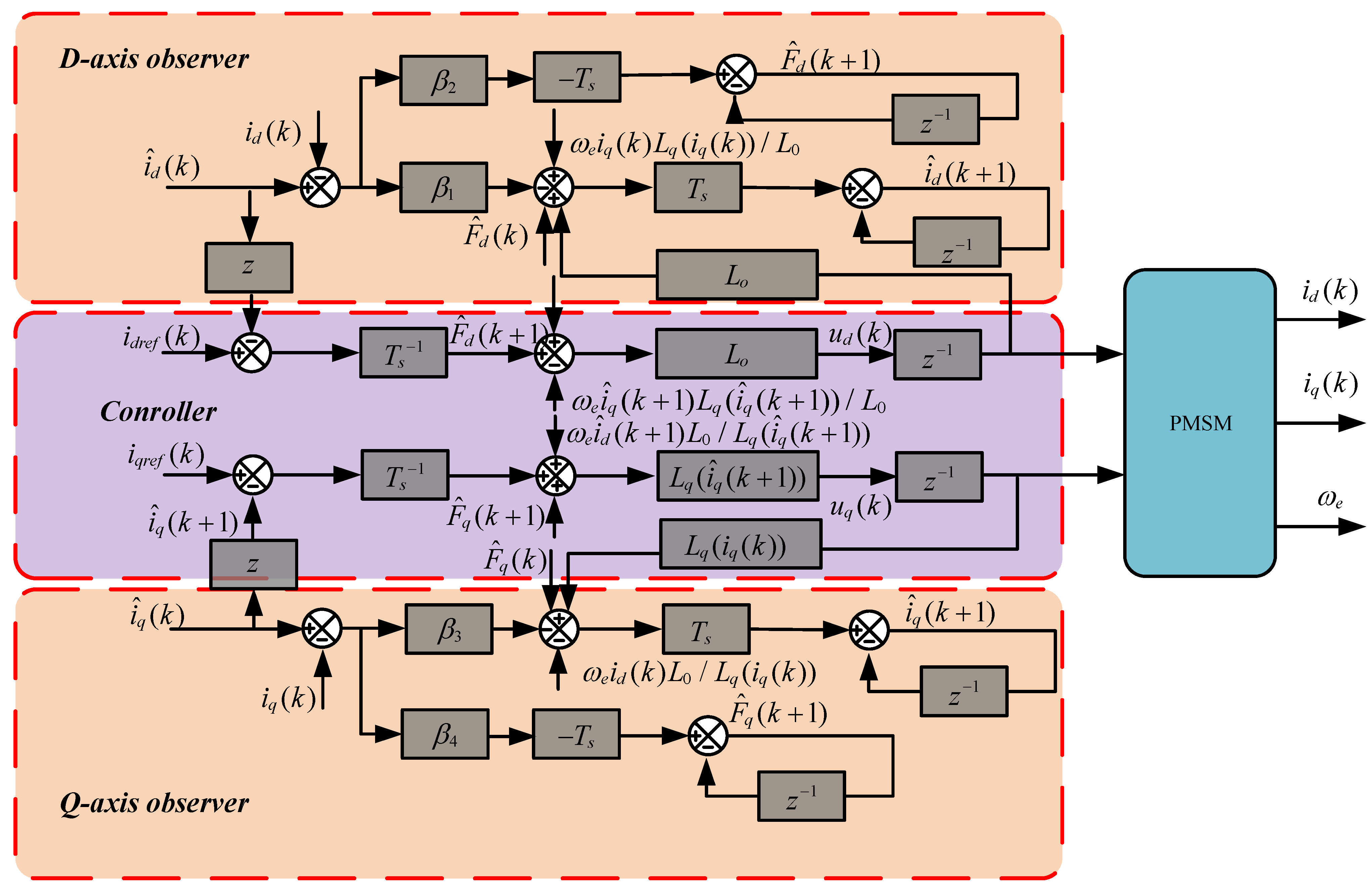
3.2. Proposed FRRDBPCC Method

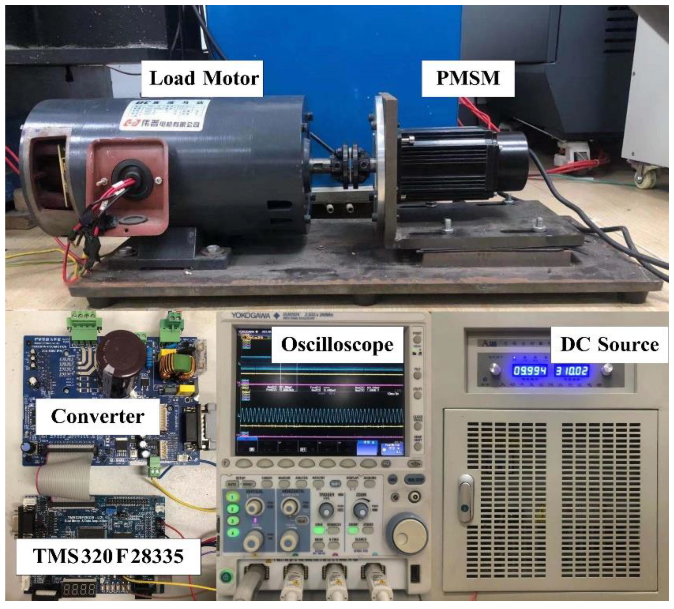
In order to achieve better current tracking performance, FRRDBPCC method considering the magnetic saturation and the cross-coupling effect of dq-axis currents is proposed, which is shown in Figure 2. The block diagram of the controller is shown in Figure 3. Considering that the values of resistance and flux linkage are mainly affected by temperature, while the change rate of ${\omega }_e{\psi }_f$ is much lower compared with the current loop and the voltage drop on the resistance is relatively small, so the current errors caused by them can be compensated by the observer.

Thus, the discrete form of the proposed FRRDBPCC can be written as:

$$\{\begin{array}{l}{\widehat{i}}_d(k+1)-{\widehat{i}}_d\left(k\right)=T_s{\omega }_e\left(k\right)i_q\left(k\right)L_q\left(i_q\left(k\right)\right)/L_0+T_s{u}_d\left(k-1\right)/L_0+T_s{\widehat{F}}_d\left(k\right)-T_s{\beta }_1\left({\widehat{i}}_d\left(k\right)-i_d\left(k\right)\right)\hfill \\ {\widehat{F}}_d(k+1)-{\widehat{F}}_d\left(k\right)=-T_s{\beta }_2\left({\widehat{i}}_d\left(k\right)-i_d\left(k\right)\right)\hfill \\ {\widehat{i}}_q(k+1)-{\widehat{i}}_q\left(k\right)=-T_s{\omega }_e\left(k\right)i_d\left(k\right)L_0/L_q\left(i_q\left(k\right)\right)+T_s{u}_q\left(k-1\right)/L_q\left(i_q\left(k\right)\right)+T_s{\widehat{F}}_q\left(k\right)-T_s{\beta }_3\left({\widehat{i}}_q\left(k\right)-i_q\left(k\right)\right)\hfill \\ {\widehat{F}}_q(k+1)-{\widehat{F}}_q\left(k\right)=-T_s{\beta }_4\left({\widehat{i}}_q\left(k\right)-i_q\left(k\right)\right)\hfill \end{array}$$

(39)

$$\{\begin{array}{c}{i}_{dref}(k)-{\widehat{i}}_d\left(k+1\right)=T_s{\omega }_e\left(k\right){\widehat{i}}_q\left(k+1\right)L_q\left({\widehat{i}}_q\left(k+1\right)\right)/L_0+T_s{u}_d\left(k\right)/L_0+T_s{\widehat{F}}_d\left(k+1\right)\\ i_{qref}(k)-{\widehat{i}}_q\left(k+1\right)=-T_s{\omega }_e\left(k\right){\widehat{i}}_d\left(k+1\right)L_0/L_q\left({\widehat{i}}_q\left(k+1\right)\right)+T_s{u}_q\left(k\right)/L_q\left({\widehat{i}}_q\left(k+1\right)\right)+T_s{\widehat{F}}_q\left(k+1\right)\end{array}$$

(40)

In order to prove the effectiveness of the proposed method, considering that in practical applications the q-axis inductance generally does not change abruptly in one step, then it can be assumed that $L_q(k)\approx L_q\left({\widehat{i}}_q\left(k+1\right)\right)$. Applying the z-transform to Equations (3), (39) and (40), ignoring the influence of resistance and considering ${\omega }_e(k){\psi }_f$ as a constant external disturbance, then it derives:

$$\{\begin{array}{l}{i}_d(z)=z^{-2}{i}_{dref}(z)\\ i_q(z)=z^{-2}{i}_{qref}(z)\end{array}$$

(41)

Compared with Equation (26), two poles of Equation (41) are both located at zero which means that the current would reach to the reference value in two periods. Meanwhile, the stability of the current control loop does not depend on the observer gain and the speed of the motor, which greatly improves the stability range of the system. Also, the steady state tracking error caused by resistance and flux linkage error will be compensated by the observer. Thus, the stability and control performance both in steady state and transient state of the proposed method are guaranteed. In this paper, ${\omega }_0$ is chosen as 3000 (rad/s).

4. Experiments

To verify the effectiveness of the proposed method, the experiments are conducted in this section. The experimental platform is shown in Figure 4. The platform includes a DC power source, a SPMSM tow system, an oscilloscope, a controlling board and a driving board. The parameters of the SPMSM control system are listed in

Table 1. Parameters of SPMSM control system.

Parameters	Value
Rated speed	1500 r/min
Pole pairs	4
Rated current	3 A
Rated torque	1.68 N.m
Rotor flux	0.09357 Wb
Stator resistance	1.75 Ω
Stator inductance	3.2 mH
DC bus voltage	310 V
Control period	100 μs

. The digital signal processor used in this paper is a TMS320F28335, of which the clock frequency is 150 MHz. The sampling frequency used in the experiment is 10 kHz, which is also the frequency of the current loop. IKCM30F60GA-type IPM is selected as the power device in the driving board. The parameters of the control system are presented in Table 1. The parameters of the speed loop PI are chosen as $k_p=0.01$, $k_i=0.0002$. The speed loop is operating at a frequency of 1 kHz.

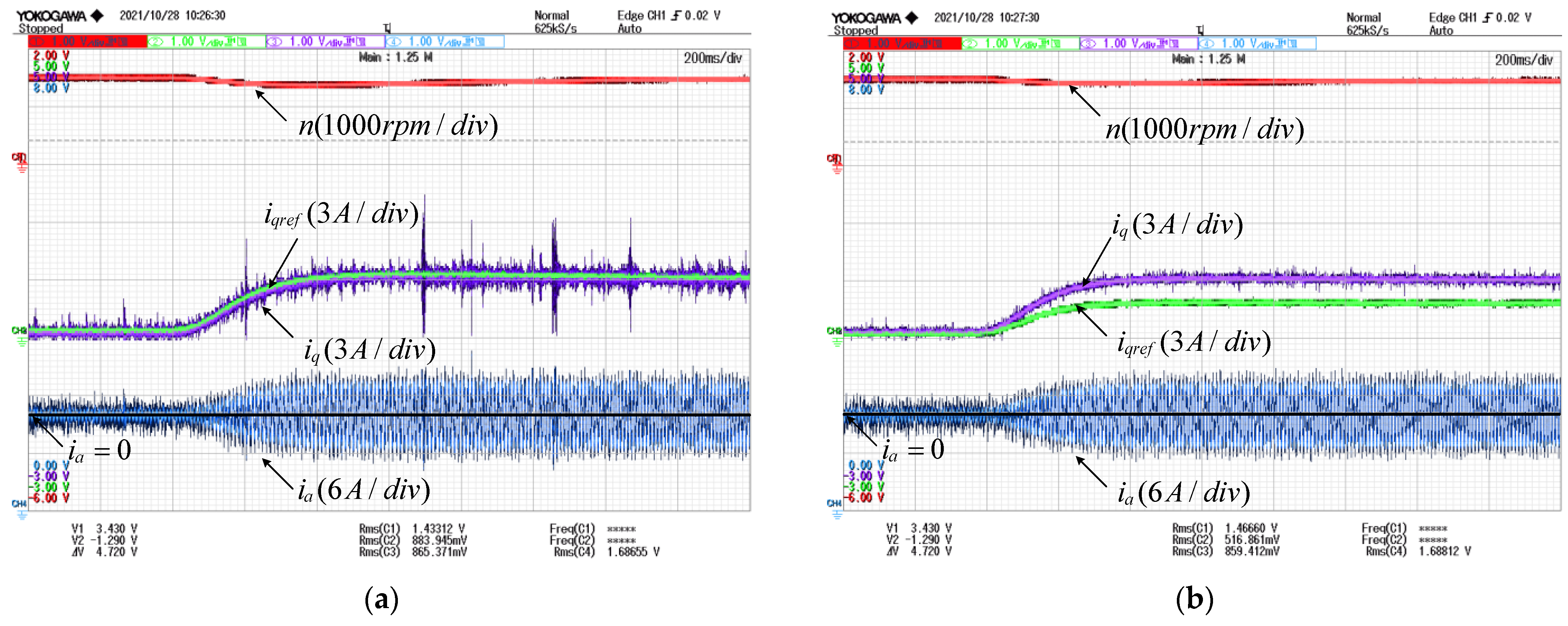
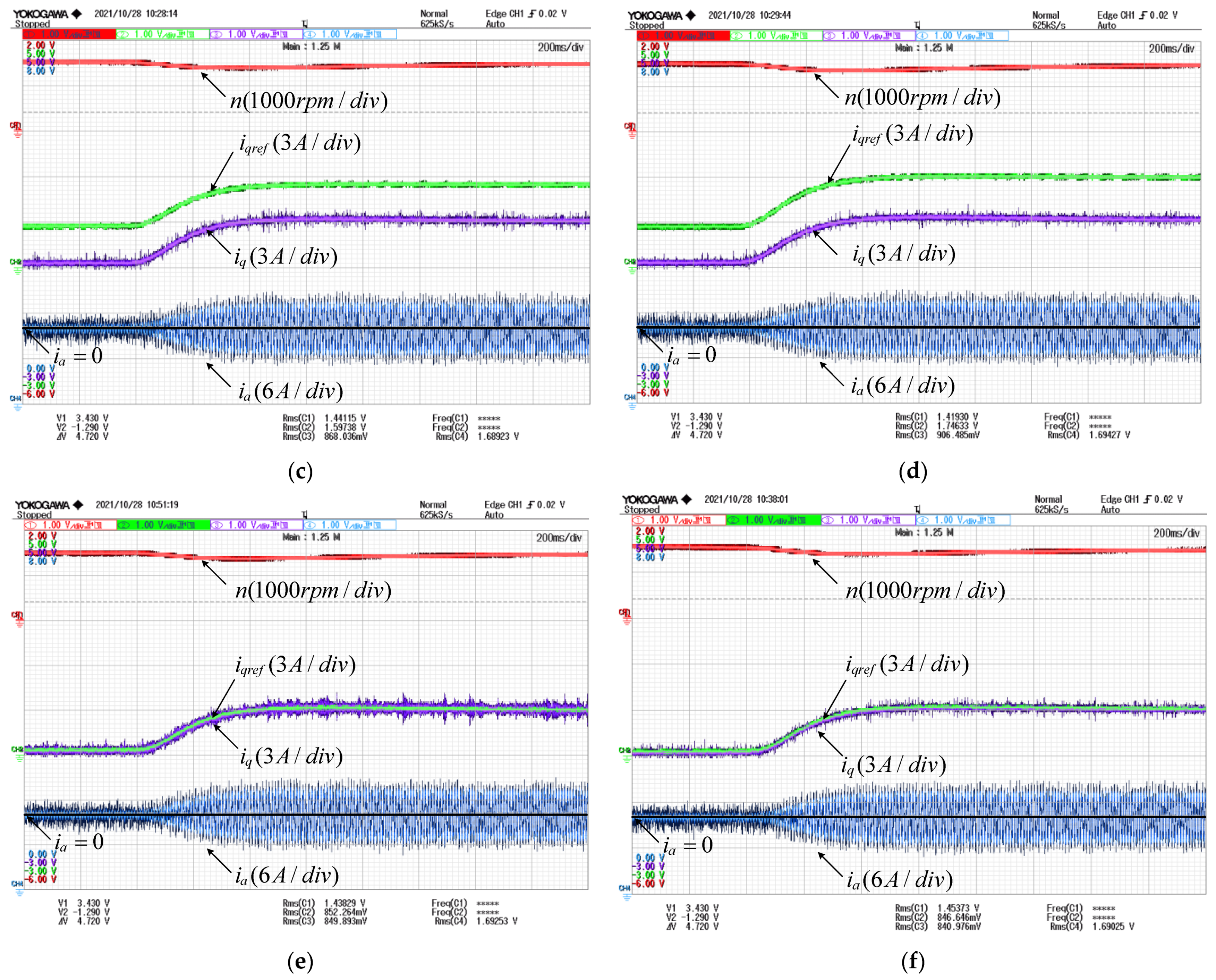
4.1. Tracking Performance of Current under Loads

Figure 5 presents the current tracking performance when the load torque is changed from 0 N.m to 1.68 N.m. The reference speed remains 1500 rpm. There is some current tracking error in the conventional DBPCC when parameter mismatch exists, which does not appear in the proposed FRRDBPCC. The PI controller shows similar performance in terms of tracking reference current with FRRDBPCC but the current ripple is worse than that of FRRDBPCC.

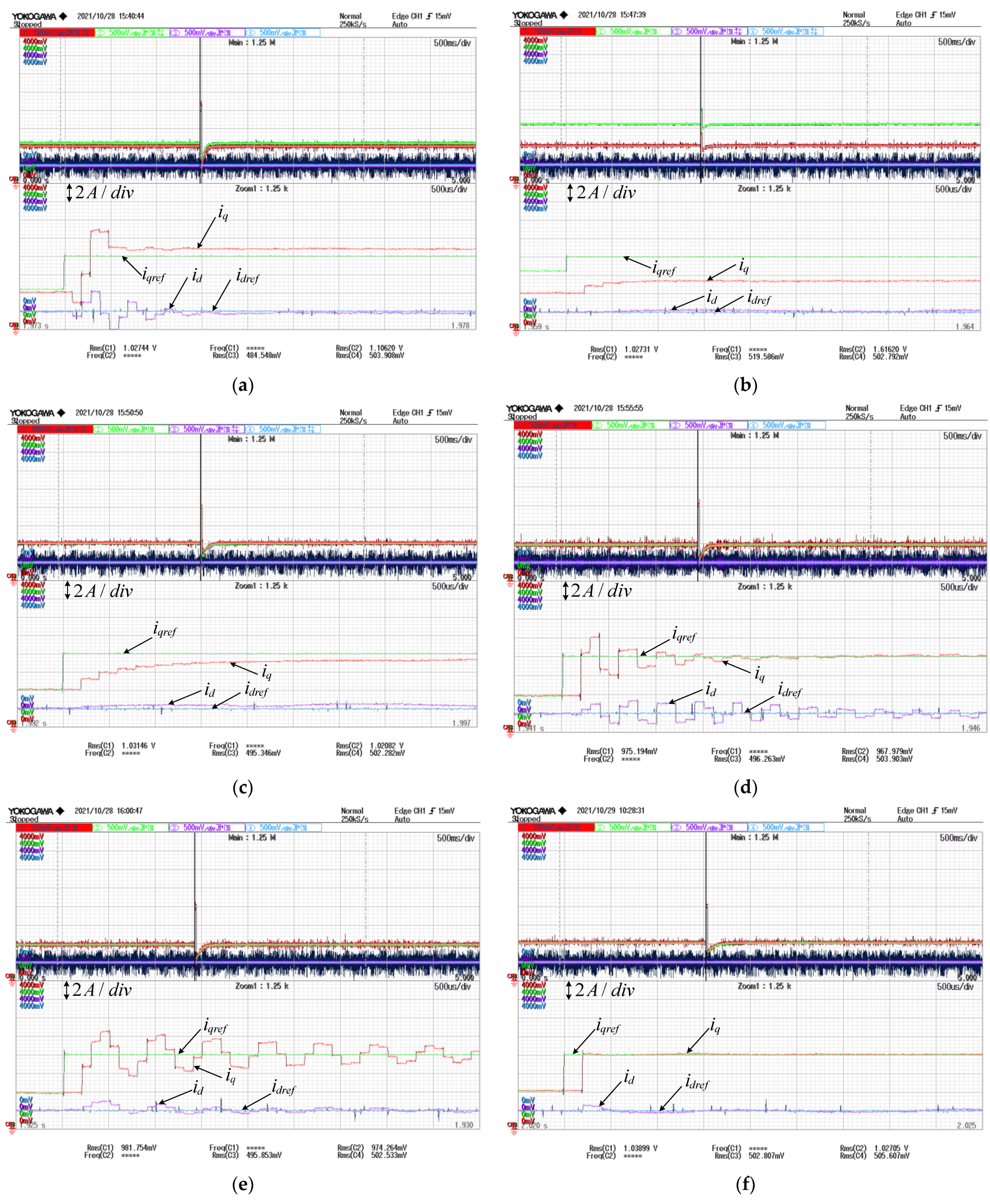
4.2. Tracking Performance of Current under Step Response

Figure 6 presents the current tracking performance when the q-axis reference current is suddenly changed to 6A. The motor operated in steady state at 1500 rpm before the sudden change of q-axis reference current. The load torque is 1.12 N.m. The comparison is listed in

Table 2. Comparison between conventional method and proposed method.

Methods	Time to Reach Steady State	Steady State Tracking Error	Cross Coupling Effect	Chatteringand Overshoot
Conventional DBPCC with $L_0=1.75L$, $R_0=5R$, ${\psi }_{f0}=0.3{\psi }_f$	0.5 ms	large	serious	serious
Conventional ESO-based DBPCC with $L_0=0.5L$, $R_0=0.1R$, ${\psi }_{f0}=0.6{\psi }_f$	0.6 ms	large	medium	no
ESO-based DBPCC with $L_0=0.3L$	2.5 ms	no	serious	no
ESO-based DBPCC with $L_0=1.55L$	2 ms	no	serious	serious
PI controller	>3 ms	no	serious	serious
FRRDBPCC	0.2 ms	no	slight	no

. In Figure 6a,b, both steady state tracking error and transient state tracking error occur in conventional DBPCC when parameter mismatch exists. In Figure 6c–e, conventional ESO-based DBPCC and PI controller can track the reference current without error in steady state. However, due to the mismatch of nominal inductance, the current tracking performance of conventional ESO-based DBPCC under step response is severely degraded. The PI controller also has a large overshoot and chattering in the current step response, and it takes a long time to converge to the reference value. Additionally, dq-axis currents suffer significantly from the cross-coupling effect in the above five cases, which deteriorates the control performance of the current loop. In Figure 6f, the proposed FRRDBPCC can track the reference current in two control periods without tracking error and completely decouple the dq-axis currents, so as to obtain the optimal current loop control performance. Thus, the effectiveness of the proposed FRRDBPCC in achieving quick dynamic response is confirmed.

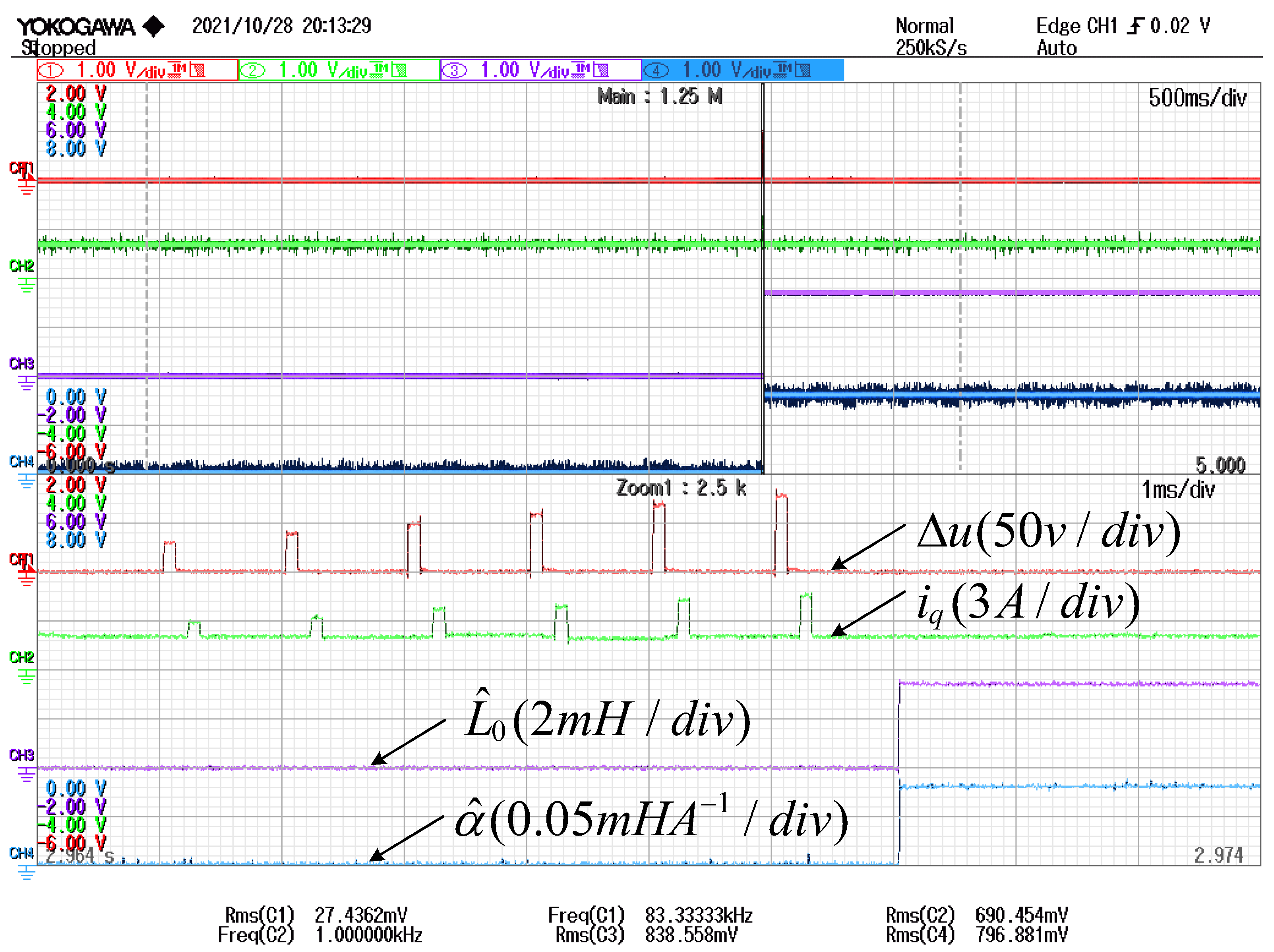
4.3. Inductance Identification

Figure 7 shows the experiment results of inductance identification. In the experiment, the motor operated in steady state at 1500 rpm and the load torque is 1.12 N.m. The amplitude of the first voltage pulse injected was 10% of the rated voltage of the motor, increasing 10 V each time. When the current was close to twice the rated current, the voltage injection was stopped. In order to reduce the estimation deviation caused by sampling error, multiple groups of experiments were repeated. Since the proposed method does not depend on the current loop controller, it is easily implemented. Finally, the results obtained by identification are $\widehat{\alpha }=0.08$ mHA⁻¹, ${\widehat{L}}_0=3.429$ mH.

5. Conclusions

This article has proposed a FRRDBPCC method for SPMSM. The major contributions of this article include the following:

(1)

An ESO is proposed to estimate the lumped disturbance. The stability and tracking performance of the current loop are analyzed in detail.

(2)

An online inductance identification algorithm considering saturation is proposed to improve the dynamic response of the current loop.

(3)

An improved prediction model is proposed. The dq-axis can be completely decoupled. The motor resistance and flux linkage are excluded in the proposed model which simplifies the selection of parameters and reduces the computation burden in digital implementation.

The conventional DBPCC method, ESO-based DBPCC method with inductance error, PI controller and the proposed FRRDBPCC method are compared by experimental results. The results show that the proposed FRRDBPCC method can track the reference value in two control periods without tracking error which ensures the transient state and steady state performance of the current loop simultaneously. For future work, the proposed ESO-based deadbeat predictive control method can be applied in the speed loop to improve its dynamic response.

References

1. Jung, J.-W.; Leu, V.Q.; Do, T.D.; Kim, E.-K.; Choi, H.H. Adaptive PID Speed Control Design for Permanent Magnet Synchronous Motor Drives. IEEE Trans. Power Electron. 2015, 30, 900–908. [Google Scholar] [CrossRef]
2. Ali, M.N.; Soliman, M.; Mahmoud, K.; Guerrero, J.M.; Lehtonen, M.; Darwish, M.M.F. Resilient Design of Robust Multi-Objectives PID Controllers for Automatic Voltage Regulators: D-Decomposition Approach. IEEE Access 2021, 9, 106589–106605. [Google Scholar] [CrossRef]
3. Qu, L.; Qiao, W.; Qu, L. Active-Disturbance-Rejection-Based Sliding-Mode Current Control for Permanent-Magnet Synchronous Motors. IEEE Trans. Power Electron. 2021, 36, 751–760. [Google Scholar] [CrossRef]
4. Chen, Q.; Yu, X.; Sun, M.; Wu, C.; Fu, Z. Adaptive Repetitive Learning Control of PMSM Servo Systems with Bounded Nonparametric Uncertainties: Theory and Experiments. IEEE Trans. Ind. Electron. 2021, 68, 8626–8635. [Google Scholar] [CrossRef]
5. Huang, M.; Deng, Y.; Li, H.; Wang, J. Torque Ripple Suppression of PMSM Using Fractional-Order Vector Resonant and Robust Internal Model Control. IEEE Trans. Transp. Electrif. 2021, 7, 1437–1453. [Google Scholar] [CrossRef]
6. Niu, S.; Luo, Y.; Fu, W.; Zhang, X. Robust Model Predictive Control for a Three-Phase PMSM Motor With Improved Control Precision. IEEE Trans. Ind. Electron. 2021, 68, 838–849. [Google Scholar] [CrossRef]
7. Petkar, S.G.; Eshwar, K.; Thippiripati, V.K. A Modified Model Predictive Current Control of Permanent Magnet Synchronous Motor Drive. IEEE Trans. Ind. Electron. 2021, 68, 1025–1034. [Google Scholar] [CrossRef]
8. Wang, F.; He, L. FPGA-Based Predictive Speed Control for PMSM System Using Integral Sliding-Mode Disturbance Observer. IEEE Trans. Ind. Electron. 2021, 68, 972–981. [Google Scholar] [CrossRef]
9. Wu, M.; Sun, X.; Zhu, J.; Lei, G.; Guo, Y. Improved Model Predictive Torque Control for PMSM Drives Based on Duty Cycle Optimization. IEEE Trans. Magn. 2021, 57, 1–5. [Google Scholar] [CrossRef]
10. Elsisi, M.; Mahmoud, K.; Lehtonen, M.; Darwish, M.M.F. Effective Nonlinear Model Predictive Control Scheme Tuned by Improved NN for Robotic Manipulators. IEEE Access 2021, 9, 64278–64290. [Google Scholar] [CrossRef]
11. Zhou, Z.; Xia, C.; Shi, T.; Geng, Q. Model Predictive Direct Duty-Cycle Control for PMSM Drive Systems With Variable Control Set. IEEE Trans. Ind. Electron. 2021, 68, 2976–2987. [Google Scholar] [CrossRef]
12. Liu, X.; Zhou, L.; Wang, J.; Gao, X.; Li, Z.; Zhang, Z. Robust Predictive Current Control of Permanent-Magnet Synchronous Motors With Newly Designed Cost Function. IEEE Trans. Power Electron. 2020, 35, 10778–10788. [Google Scholar] [CrossRef]
13. Wang, F.; Zuo, K.; Tao, P.; Rodriguez, J. High Performance Model Predictive Control for PMSM by Using Stator Current Mathematical Model Self-Regulation Technique. IEEE Trans. Power Electron. 2020, 35, 13652–13662. [Google Scholar] [CrossRef]
14. Wang, F.; He, L.; Rodriguez, J. FPGA-Based Continuous Control Set Model Predictive Current Control for PMSM System Using Multistep Error Tracking Technique. IEEE Trans. Power Electron. 2020, 35, 13455–13464. [Google Scholar] [CrossRef]
15. Wei, Y.; Wei, Y.; Sun, Y.; Qi, H.; Guo, X. Prediction Horizons Optimized Nonlinear Predictive Control for Permanent Magnet Synchronous Motor Position System. IEEE Trans. Ind. Electron. 2020, 67, 9153–9163. [Google Scholar] [CrossRef]
16. Elsisi, M.; Tran, M.-Q.; Mahmoud, K.; Lehtonen, M.; Darwish, M.M.F. Robust Design of ANFIS-Based Blade Pitch Controller for Wind Energy Conversion Systems Against Wind Speed Fluctuations. IEEE Access 2021, 9, 37894–37904. [Google Scholar] [CrossRef]
17. Yuan, X.; Zhang, S.; Zhang, C. Enhanced Robust Deadbeat Predictive Current Control for PMSM Drives. IEEE Access 2019, 7, 148218–148230. [Google Scholar] [CrossRef]
18. Zhang, X.; Hou, B.; Mei, Y. Deadbeat Predictive Current Control of Permanent-Magnet Synchronous Motors with Stator Current and Disturbance Observer. IEEE Trans. Power Electron. 2017, 32, 3818–3834. [Google Scholar] [CrossRef]
19. Yang, J.; Chen, W.-H.; Li, S.; Guo, L.; Yan, Y. Disturbance/Uncertainty Estimation and Attenuation Techniques in PMSM Drives—A Survey. IEEE Trans. Ind. Electron. 2017, 64, 3273–3285. [Google Scholar] [CrossRef] [Green Version]
20. Wang, B.; Chen, X.; Yu, Y.; Wang, G.; Xu, D. Robust Predictive Current Control With Online Disturbance Estimation for Induction Machine Drives. IEEE Trans. Power Electron. 2017, 32, 4663–4674. [Google Scholar] [CrossRef]
21. Jiang, Y.; Xu, W.; Mu, C.; Liu, Y. Improved Deadbeat Predictive Current Control Combined Sliding Mode Strategy for PMSM Drive System. IEEE Trans. Veh. Technol. 2018, 67, 251–263. [Google Scholar] [CrossRef]
22. Sun, X.; Cao, J.; Lei, G.; Guo, Y.; Zhu, J. A Robust Deadbeat Predictive Controller With Delay Compensation Based on Composite Sliding-Mode Observer for PMSMs. IEEE Trans. Power Electron. 2021, 36, 10742–10752. [Google Scholar] [CrossRef]
23. Gong, Z.; Zhang, C.; Ba, X.; Guo, Y. Improved Deadbeat Predictive Current Control of Permanent Magnet Synchronous Motor Using a Novel Stator Current and Disturbance Observer. IEEE Access 2021, 9, 142815–142826. [Google Scholar] [CrossRef]
24. Zhang, Y.; Jin, J.; Huang, L. Model-Free Predictive Current Control of PMSM Drives Based on Extended State Observer Using Ultralocal Model. IEEE Trans. Ind. Electron. 2021, 68, 993–1003. [Google Scholar] [CrossRef]
25. Xu, L.; Chen, G.; Li, Q. Ultra-Local Model-Free Predictive Current Control Based on Nonlinear Disturbance Compensation for Permanent Magnet Synchronous Motor. IEEE Access 2020, 8, 127690–127699. [Google Scholar] [CrossRef]
26. He, L.; Wang, F.; Wang, J.; Rodriguez, J. Zynq Implemented Luenberger Disturbance Observer Based Predictive Control Scheme for PMSM Drives. IEEE Trans. Power Electron. 2020, 35, 1770–1778. [Google Scholar] [CrossRef]
Figure 1. Close loop zeros and poles vary with speed, nominal inductance and observer gain. (a) ω e = 400 ,   L 0 = 0.3 L ; (b) ω e = 400 ,   L 0 = L ; (c) ω e = 400 ,   L 0 = 2 L ; (d) ω e = 1000 ,   L 0 = 0.3 L ; (e) ω e = 1000 ,   L 0 = L ; (f) ω e = 1000 ,   L 0 = 2 L ; (g) ω e = 2000 ,   L 0 = 0.3 L ; (h) ω e = 2000 ,   L 0 = L ; (i) ω e = 2000 ,   L 0 = 2 L .
Energies 14 07563 g001
Figure 2. Block diagram of the proposed method.
Energies 14 07563 g002
Figure 3. Block diagram of the FRRDBPCC.
Energies 14 07563 g003
Figure 4. The experimental platform.
Energies 14 07563 g004
Figure 5. Experiment results of current tracking performance under loads. (a) Conventional DBPCC with L 0 = 1.8 L ; (b) conventional DBPCC with R 0 = 6 R ; (c) conventional DBPCC with ψ f 0 = 0.3 ψ f ; (d) conventional DBPCC with L 0 = 0.6 L , R 0 = 0.1 R , ψ f 0 = 0.6 ψ f ; (e) PI controller; (f) FRRDBPCC.
Energies 14 07563 g005aEnergies 14 07563 g005b
Figure 6. Experiment results of current tracking performance under step response. (a) Conventional DBPCC with L 0 = 1.75 L , R 0 = 5 R , ψ f 0 = 0.3 ψ f ; (b) conventional DBPCC with L 0 = 0.5 L , R 0 = 0.1 R , ψ f 0 = 0.6 ψ f ; (c) ESO-based DBPCC with L 0 = 0.3 L ; (d) ESO-based DBPCC with L 0 = 1.55 L ; (e) PI controller; (f) FRRDBPCC.
Energies 14 07563 g006
Figure 7. Experiment results of inductance identification.
Energies 14 07563 g007