Abstract
Forecasting Photovoltaic (PV) energy production, based on the last weather and power data only, can obtain acceptable prediction accuracy in short-time horizons. Numerical Weather Prediction (NWP) systems usually produce free forecasts of the local cloud amount each 6 h. These are considerably delayed by several hours and do not provide sufficient quality. A Differential Polynomial Neural Network (D-PNN) is a recent unconventional soft-computing technique that can model complex weather patterns. D-PNN expands the n-variable kth order Partial Differential Equation (PDE) into selected two-variable node PDEs of the first or second order. Their derivatives are easy to convert into the Laplace transforms and substitute using Operator Calculus (OC). D-PNN proves two-input nodes to insert their PDE components into its gradually expanded sum model. Its PDE representation allows for the variability and uncertainty of specific patterns in the surface layer. The proposed all-day single-model and intra-day several-step PV prediction schemes are compared and interpreted with differential and stochastic machine learning. The statistical models are evolved for the specific data time delay to predict the PV output in complete day sequences or specific hours. Spatial data from a larger territory and the initially recognized daily periods enable models to compute accurate predictions each day and compensate for unexpected pattern variations and different initial conditions. The optimal data samples, determined by the particular time shifts between the model inputs and output, are trained to predict the Clear Sky Index in the defined horizon.
1. Introduction
Accurate forecasting of hourly or daily solar radiation or direct PV Power (PVP) is challenging, as it is influenced by complex dynamic processes combined with irregular fluctuations resulting in local anomalies [1]. NWP systems model atmospheric 3D circulation in several layers. Their physical airflow models are naturally less sensitive to specifics in the near-ground boundaries; therefore, sophisticated post-processing is unavoidable [2]. Artificial Intelligence (AI) techniques, using historical time series, attempt to model local patterns and predict intra-day stochastic PVP supplies taking into account the previous case states [3]. This statistical approach can also be used to post-process the corresponding NWP output in 24–48 h prediction series [4]. Historical solar irradiation input and target PVP output samples over pre-estimated day-periods can be learned to develop daily statistical AI models [5]. The 24 or 48 h local forecasts of a regional NWP model are then processed to compensate for the unavailable observations in the calculation of the PVP output series at the corresponding times [6]. However, this PVP prediction strategy based on converted local solar radiation forecasts is largely dependent on the quality of processed NWP data. AI applications can suffer some limitations, e.g., over-fitting, excessive simplification, deep matching of the models to specific criteria, etc. The iterative learning procedure, e.g., using an Artificial Neural Network (ANN), beginning with randomly weighted parameters, can yield different estimations. The definite model is usually a weighted ensemble that rates individual solutions or is calculated using a time-probabilistic approach, taking into account the test specifics [7].
The designed bio-inspired D-PNN automatically splits the linear kth order PDE of n-variables into two-input node PDEs applying the polynomial OC conversion to form the rational functions. A self-adapting algorithm develops the growing tree-frame of the Polynomial Neural Network (PNN) to produce successive partial sub-PDE models in the extended D-PNN structure [8]. The inverse Laplace transformation (L-transform) using complex variables based on the representation of Complex Neural Networks (CNN) and OC statements is used to produce node PDE components included in the output sum model. Progressive PNN growth results in the extension PDE model using Goeddel’s incompleteness theorem, which mainly enables the best interpretation of data patterns (Section 3). D-PNN overcomes the problems of signal preprocessing and feature determination, applying the Laplace transformation to PDE derivatives and effective selection of two-node input variables using PNN. Its self-examination of two-input nodes according to the significant data relations using extending tree-layer back-composing architecture is related to the convolution principles of Deep Learning (DL).
Test predetermined sequences of applicable training records, based on the pattern similarity with observations in the latest hours, are originally recognized by auxiliary models. The identified optimal daily data samples are trained for particular inputs->output time delays (Section 4). The resulting models are applied after competent testing to the last observed series of data to calculate the PVP output in the corresponding training-defined horizon (Section 5). The proposed one-day and single-time prediction strategies allow development of the optimal models in consideration of an adequate quality, practicability and processing complexity in relation to historical training and oncoming weather patterns. Changeable conditions, unexpected abnormalities or undefined states can result in alterative usefulness and efficiency of both the compared statistical approaches, which can be combined and implemented for various PVP plant specifications and configurations.
2. State of the Art in PVP Forecasting
The accuracy of PVP forecasting is primarily determined by its prediction horizon, where similar model parameters can yield different results. Prediction intervals (PI) and confidence intervals (CI) can reduce the effect of weather uncertainties and improve the efficiency of forecasting models. SIs are calculated from data statistics, while PIs define the upper and lower bounds of probability realization, providing information for future cases [9]. The spatial–temporal resolution of data influences the performance of models in the increased prediction horizon [10]. Data resampling can be applied in multi-step ahead prediction using machine learning. A new representation of the original series allows a separate model to compute its predictions at each time-step on the resampled data [11]. Ensemble empirical mode decomposition can be applied to the original PVP series under different weather conditions. The complexity of each component is reconstructed from the sample entropy to reduce computational cost [12]. The correlation of meteorological inputs and PVP output vary in different locations and greatly influences the performance of forecasting models. A strong correlation naturally exists between PVP and solar irradiance, compared to temperature and other atmospheric factors. Historical data may contain undesirable spikes and non-stationary components due to uncertain and changeable weather conditions. These anomalies and defects in regular series, which can lead to training problems and higher forecast errors, can be eliminated by preprocessing [13]. PVP prediction errors are strongly correlated with the seasonal characteristics of the irradiance error distribution in NWP. Seasonal models developed with a non-iterative algorithm can correct their forecasts [14]. The uncertainty in NWP varies with different weather conditions. Combining individual forecasting algorithms can increase the accuracy of final forecasts for the day ahead. The frequency of retraining of the forecasting model is to be determined to optimize its performance and computational burden [15]. The temporal features of data can first be extracted by the LSTM network and combined with the spatial features determined by convolutional neural network in the hybrid model based on DL [16]. Ideal and non-ideal weather types could first be recognized in the separated data samples. The relevance of time series and weather type characteristics are considered in the discrete gray model to correct the PVP prediction series [17]. The selection of NWP models has a strong effect on the accuracy of the physical prediction of PVP, as the difference is mainly related to the separation of irradiance components and the transposition of models [18]. K-means can cluster historical PVP data into groups applied by gray relational analysis for multivariate meteorological factors to determine days of similarity and optimal similarity for the forecast day [19].
Post-processing utility of NWP or statistical models can calculate the weighted output in an ensemble, taking into account the reliability of individual solutions for the recognized local weather type [20]. If the single forecasts exceed a threshold limit, their stochastic output is re-evaluated considering composed probabilistic intervals to assess the uncertainty. The boundary and starting conditions with the physical parameterizations of NWP models can greatly influence their accuracy [21]. NWP models can be compared with clear sky data to determine the optimal training samples and the number of iterations used in parameter adaptation [4]. Atmospheric transmission factor, determined by comparison between observation and NWP data, can be used as an additional model input [5]. Statistical AI computing can make use of a direct or iterative approach or combine them for the multi-step predictions. In the first one, all the outputs are forecasted at different times at once, contrary to the second iterative scheme, predicting single values, one by one, using a recursive algorithm in the next time steps [22]. Additional meteorological quantities can be tested as input to improve the performance of AI models, for example, visibility, heights of the cloudiness base or condensation output level, aerosol and turbidity coefficients, integral wind trajectory [2].
3. General PDE Partition, L-Transformation and Inverse L-Substitution
The general linear PDE of n-variables Equation (1) can be decomposed into a simplified set of PDEs that describe an unknown separable u function formulated in terms of series Equation (2) of its partial summation functions uk [23]. These items are obtained from the predefined two-variable sub-PDEs Equation (3). The L-transformation of the uk derivatives included in PDEs is first applied with their secondary inverse restoration using OC and CNN.
u(x) = f(x1, x2, …, xn) is searched separable n-variable function, a, b, c(c1, c2, …, cn), d(d11, d12, …), … are coefficients and uk are summary terms of u function
A, B, C, D, E, F, G are dependent on function u of x1, x2 input variables.
A(∂2u/∂x21) + B(∂2u/∂x1x2) + C(∂2u/∂x22) + D(∂u/∂x1) + E(∂u/∂x2) + Fu = 0
3.1. L-Transformation of PDE Derivatives and OC Iverse L-Substitution for the Rational Converts
OC conversion of an Ordinary Differential Equation (ODE) into pure rational polynomials makes use of the proposition of the applicable L-transformed nth derivatives of the function f(t) if their boundary and starting conditions are known Equation (4).
f(t), f’(t), …, f(n)(t) are continuous in the interval <0+, ∞>, t and p are their real and complex representations
The resulting rational fractions can be used to express the L-transformation of the unknown f(t) ODE function. The inverse L-transformation, using CNN and OC conversion formulas Equation (5), is necessary to recover the searched original f(t) from the ODE.
P(p) and Q(p) are s-1 and s- degree multinomials.
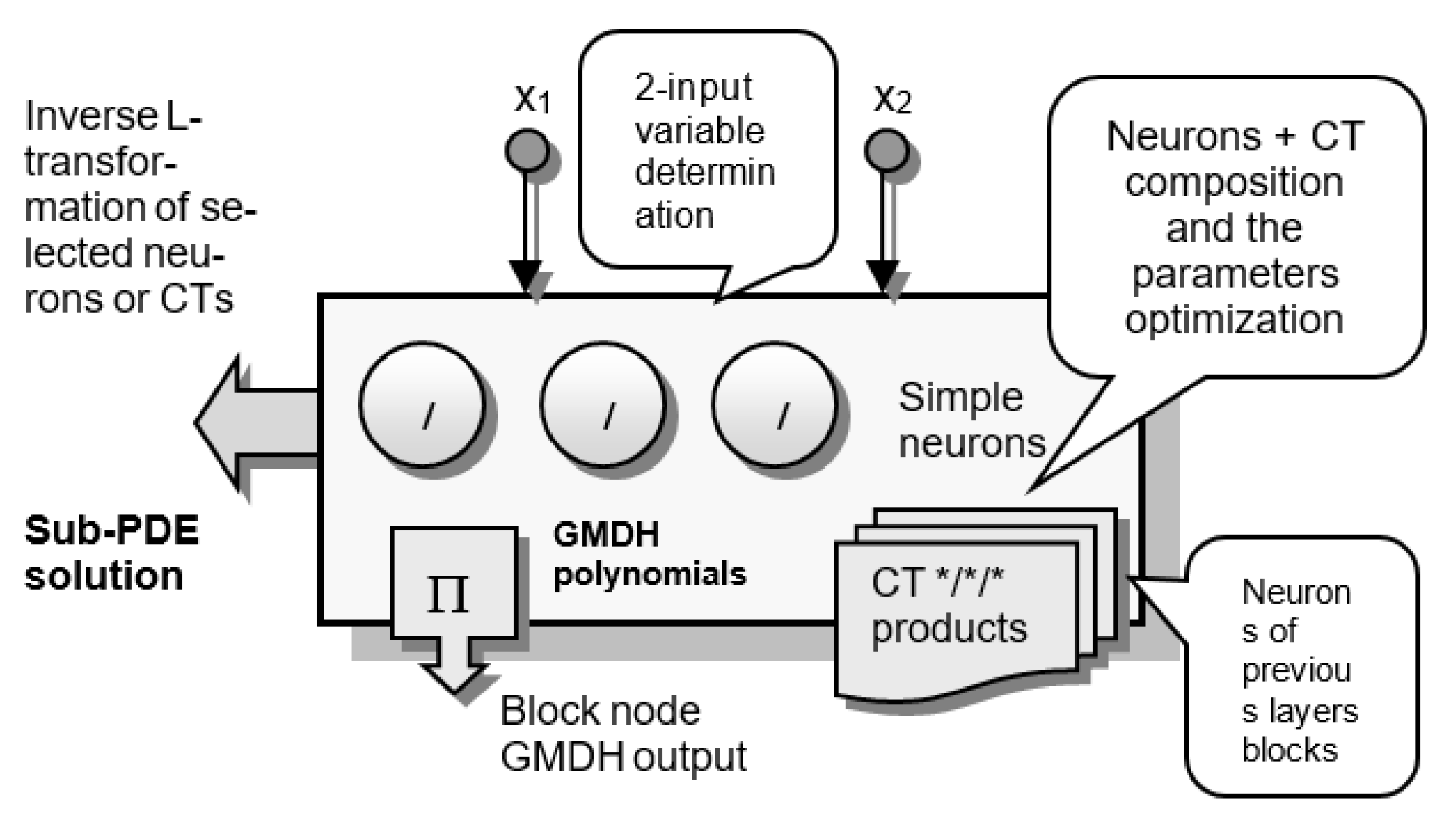
D-PNN composes applicable node rational terms, e.g., Equation (8), using GMDH multinomials Equation (6) in its PNN structure (Figure 1). It converts determined sub-PDEs Equation (3) into the L-transforms of unknown uk sum functions of two-input node variables Equation (2).
xi, xj are two-input node variables and ak are parameters.
y = a0 + a1xi + a2xj + a3xixj + a4xi2 + a5xj2

Figure 1.
Two-variable nodes are selected to produce simple or composite PDE-components solving the sub-PDEs.
The formation of sub-PDE solutions in the selected nodes Equation (7) results in a convergent sum of uk functions. The originals are produced in a two-variable PNN tree-structure (Figure 1) to compose a PDE-component model of the searched output summation u function Equation (2).
yi are composed sub-PDE solutions of searched node functions, φ = arctg(x2/x1) is the angle of two-input node variables x1, x2, sig is sigmoidal transform of squared variables and ai, bi and w are parameters and weights.
The blocks placed in PNN nodes (Figure 1) produce neurons, e.g., Equation (7), to solve specific two-variable PDEs in rational terms. The selected one is transformed inversely into the original and inserted into the sum to minimize iteratively the model output errors [23].
Complex numbers c Equation (8) are expressed in Euler polar notation, according to the principles applied in CNN, to formulate the original f(t) Equation (5).
3.2. Composite Production of PDE Model CT Components in the Progressively Extending PNN Binary Node Tree
D-PNN iteratively forms a PNN tree-framework, beginning empty and first inserting one node of the first layer only. It adds the next block nodes (Figure 1), one by one, searching for the best-fit two-inputs. These are used to produce a neuron Equation (7), i.e., a sub-PDE component, which can extend the output model. The next nodes and layers are added to the expanding PNN structure where the selected nodes produce applicable composite sub-PDE solutions to iteratively optimize the output sum model (Figure 1). This gradual expansion of PDE is expressed by the incompleteness theorem stated by Kurt Goedel: if the complexity of a model representation is increasing, the objective constraints of a problem formulation are continually decreasing (usually falling in the optima) [24]. The D-PNN multi-layer frame is developed and it can be modified dynamically (nodes added/removed) in each iteration training cycle.
k is the number of applied neurons or CTs produced by blocks in selected nodes.
D-PNN blocks in the following layer nodes can form Composite Terms (CT) in addition to neurons Equation (7). CTs are formed by the neuron products (Figure 1), i.e., OC-converted node PDEs produced in the same and back-connected blocks. Adapted neurons, or CTs, can be inserted into the overall output Y of D-PNN which is calculated as the arithmetic mean of their best single outputs yi Equation (9). Appropriate first- or second-order polynomials are applied to obtain the optimal PDE-components in the PNN nodes. This multi-step iteration algorithm skips the next or random node blocks (Figure 1), one by one, to minimize the D-PNN output error taking into account external complement testing [24].
4. Multi-Step Hourly and One-Step All-Day CSI/PVP Forecasting—Methodology
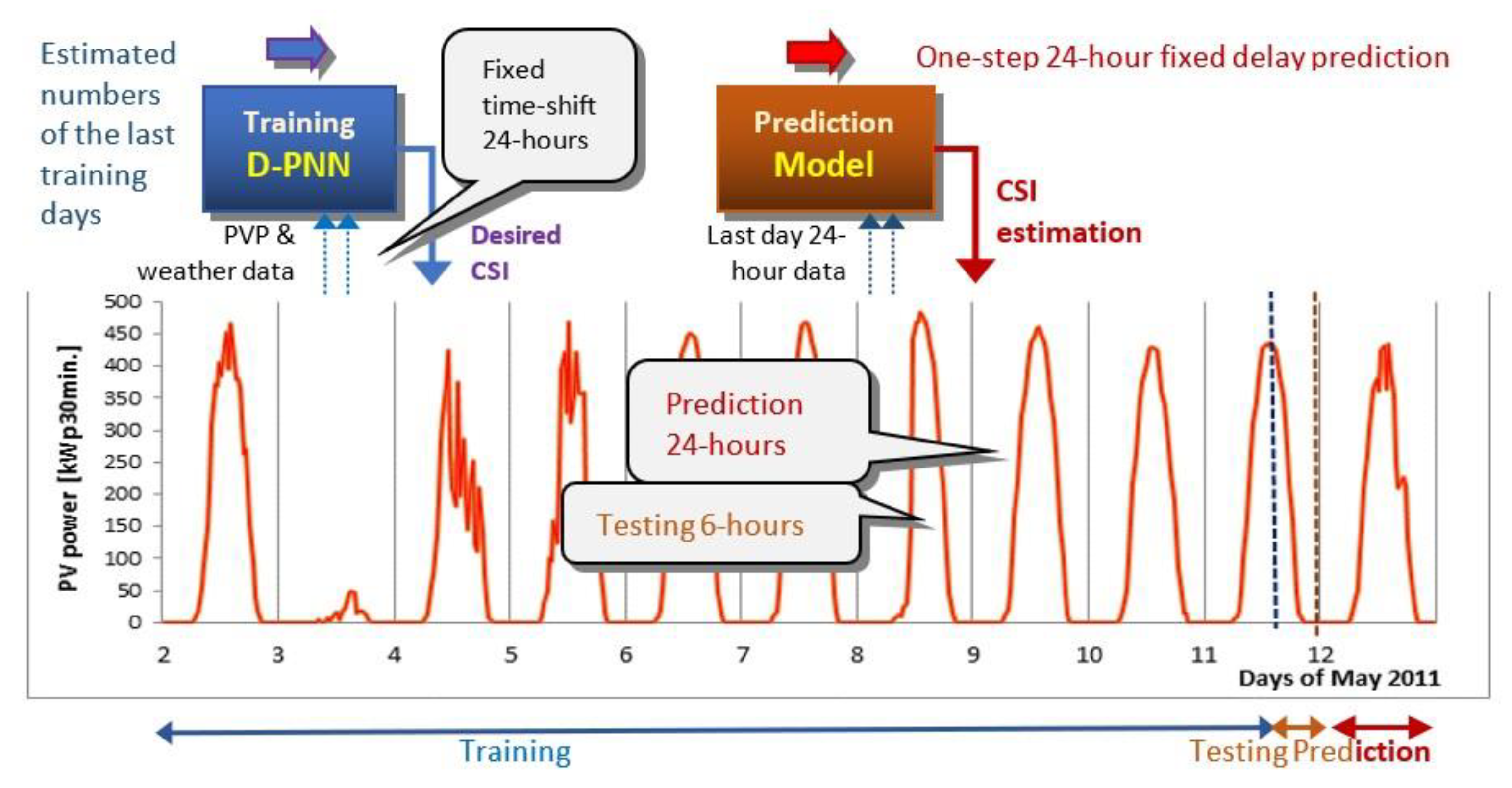
Intra-day 1–9 h models with gradually increased delay between the inputs and PVP output predict PVP at the particular hour. They process the last data from 7:30 a.m. to calculate PVP at 8 a.m.–5 p.m. in the trained time-horizon 1–9 h ahead (Figure 2). Daily models predict all data series at once, i.e., the same 24 h model is applied to the all-day 30 min data sequences to compute the following day corresponding PVP output at 6 a.m.–7:30 p.m. (Figure 3). Intra-day models use the latest input data in the same day to predict PVP in the increased time horizon, while all-day models need to reserve the last 24 h part of the data to predict the following day complete series. This approach, using a 24 h fixed time delay, is usually less precise in comparison to the more complicated multi-step intra-day procedure, forming more precisely separate models for each prediction time.
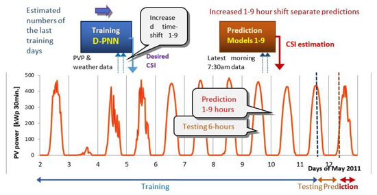
Figure 2.
Intra-day hourly PVP predictions with models using the increasing 1–9 h time-horizon between the inputs-> CSI output. Training, testing and PVP prediction for each 1–9 h using a separate model in each step.
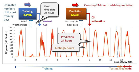
Figure 3.
Daily PVP prediction 24 h ahead using one model in one-series step.
Initial secondary models were firstly formed with data from the previous 1, 2, …, x-days to determine the lengths of daily training sequences. These simplified models are not applied in prediction, but they are only permanently tested with a reserved part of data in the last day of the afternoon. Their test error minima detect the optimal training series which usually leads to the acceptable prediction accuracy of models applied to the last available early day or all-day data. Both the all-day complete series and intra-day single hour approaches use the estimated day-intervals and the last 6 h test (Figure 3).
where, PVPclear is power in clear sky and t is time
Clear Sky Index (CSI) kt, is defined as the ratio between the actual and maximal PVP under clear sky at a time t. PVP and solar irradiation data are to be used in a standard CSI form to represent relative data no matter the diurnal period [25]. After CSI computing, the PVP output was restored from the normalized model output kt taking into account the prediction time Equation (10). Clear sky cycles can be automatically detected from the season peak daily sequences in each half hour.
5. 1–9 h and 24 h CSI/PVP Forecasting—Data and Experiments
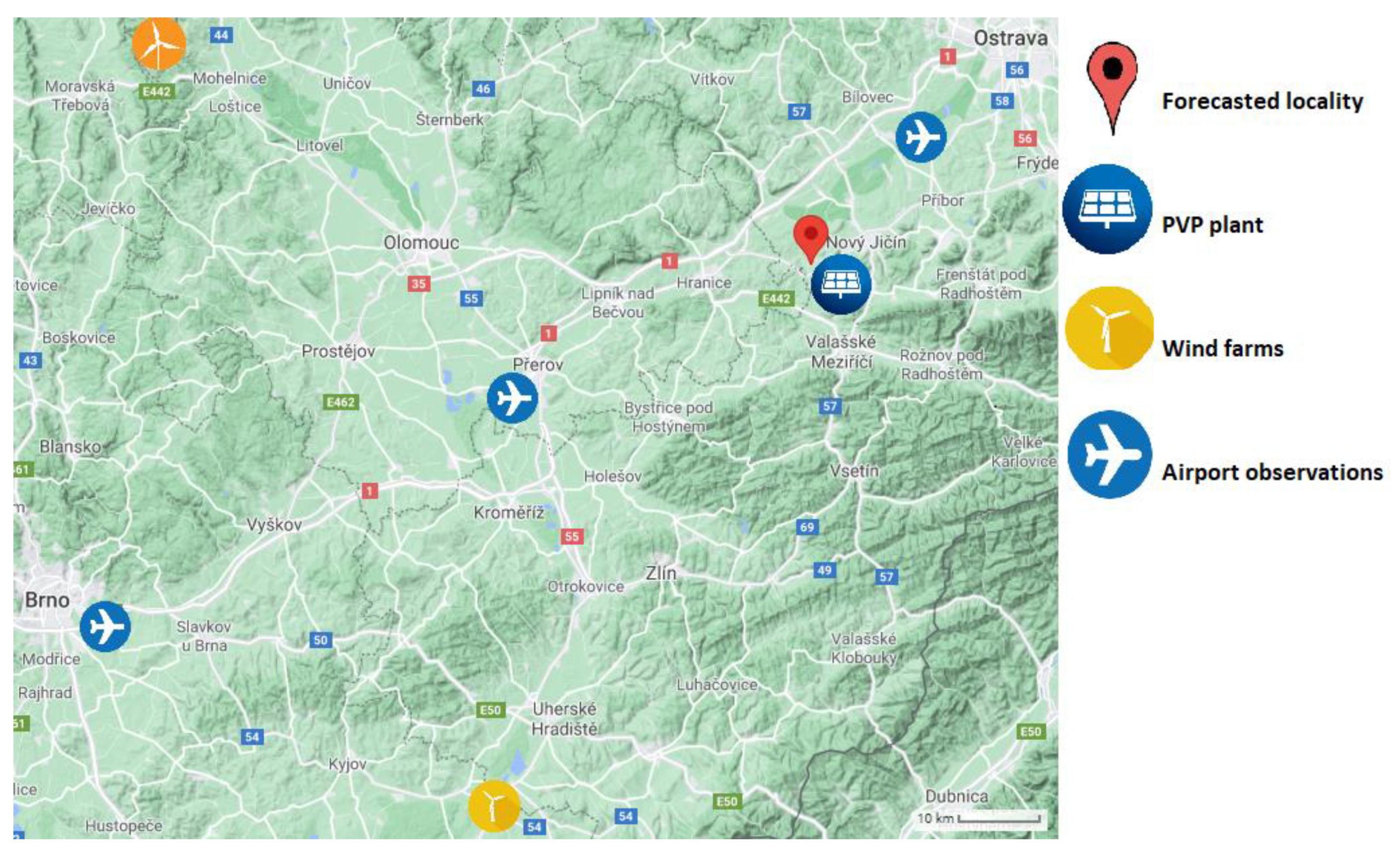
The forecast location of the PVP plant is Starojícka Lhota, Czech Republic (sea level: 332 m, longitude: 49.57°, latitude: 17.92°). Historical PVP, ground temperature and solar irradiation records were combined with wind and azimuth measurements from two local farms (locations: Veselí nad Moravou, Maletín). Additional relevant meteorological observations (avg. temperature, humidity, see pressure, wind and cloud cover conditions) from weather-ground stations of three regional airports in Ostrava (Mošnov), Brno (Tuřany) and Přerov (Bochoř, Figure 4) extended the original PVP and wind datasets (Weather underground historical data series: www.wunderground.com/history/daily/cz/mošnov/LKMT (accessed on 21 October 2021)).
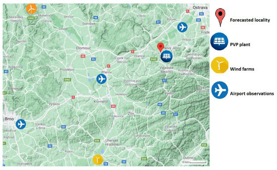
Figure 4.
The locations of predicted PVP plant, surrounding airport weather stations and wind farms (spatial data measurements and observations).
PVP, solar and wind 10 min measured data were averaged to be related to 30 min. stamped data of standard airports observations (D-PNN application C++ parametric software and Power data: https://drive.google.com/drive/folders/1ZAw8KcvDEDM-i7ifVe_hDoS35nI64-Fh?usp=sharing (accessed on 21 October 2021)). Data samples from the initially pre-assessed periods of x last days allow training the relationships in particular 1–9 or 24 h delay of the inputs–output PVP. The final models are able to process the last recorded early hour or all-day data to estimate the PVP output in the applied time-horizon (Figure 2 and Figure 3).
Table 1 shows spatial correlations between two airport and target PVP plant data measurements. The data interval <−1, 1> denotes the linear intensity dependence. Two variables are highly correlated if their coefficient of correlation leans towards +1; analogously, they are absolutely inverse correlated if the value −1 is reached. The correlation coefficient of the relative humidity and PVP data is the highest (inverse) compared to the rest of the applied input variables. Wind azimuth features the lowest correlation with PVP but it is directly coupled with wind speed, i.e., a part of the complex variable.

Table 1.
Airport and PVP plant spatial data correlations.
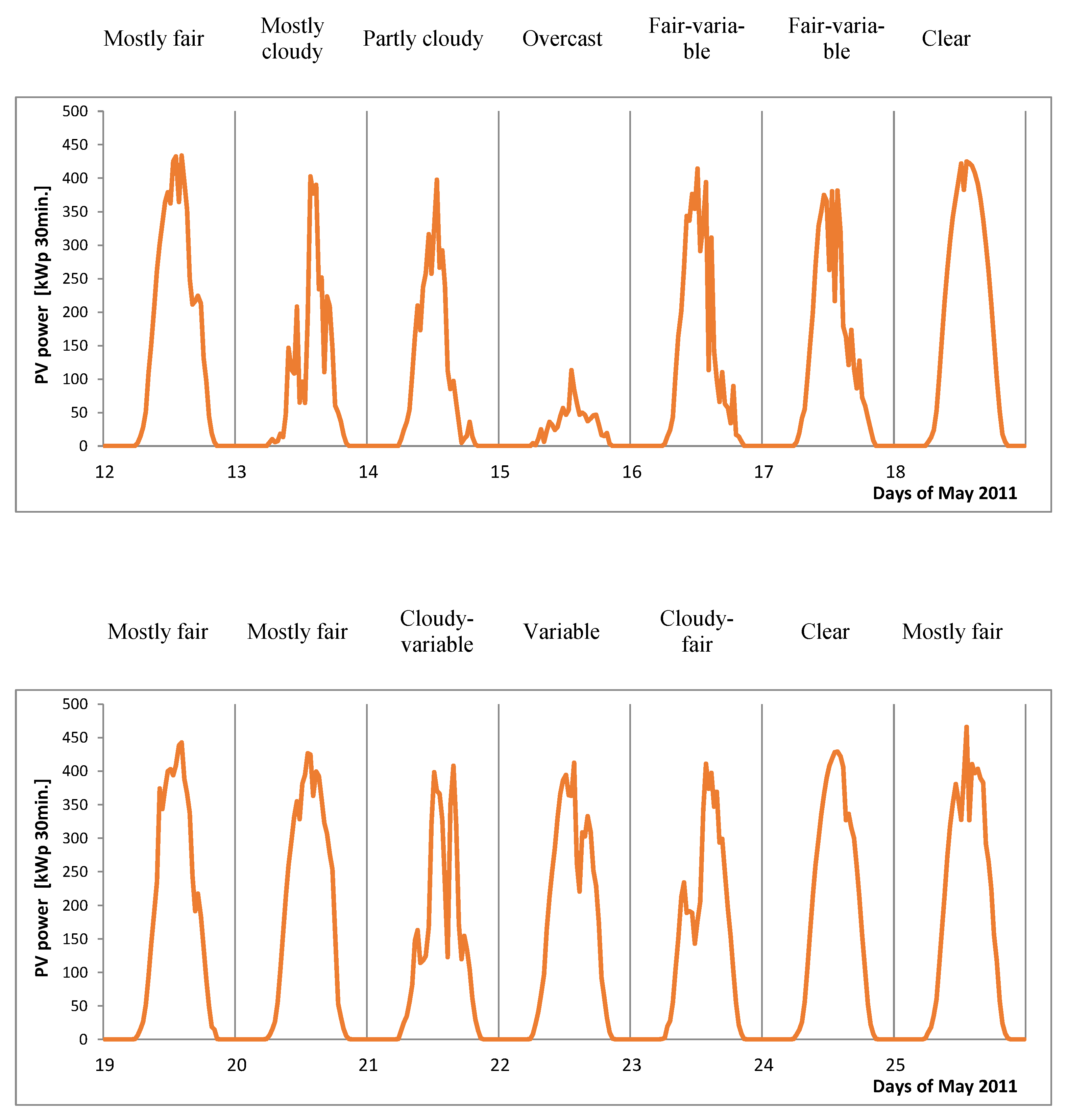
Figure 5 outlines the daily sky conditions (PVP patterns corresponding to the cloud structures and amount) in the forecasted locality in the 14-day period of interest (Weather underground historical data series: www.wunderground.com/history/daily/cz/mošnov/LKMT (accessed on 21 October 2021)).
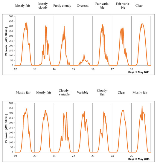
Figure 5.
Daily sky conditions (PVP cycles) in the forecasted locality (Weather underground historical data series: www.wunderground.com/history/daily/cz/mošnov/LKMT (accessed on 21 October 2021)).
A Recurrent Neural Network (RNN) with four-lagged inputs of CSI predicts the following time PVP data in sequences, making use of the hourly multi-step approach. This iterative algorithm is based on data predicted at the previous time-steps, using the values as common inputs applied successively to the model in an hourly prediction horizon. RNN consists of a layer of 20 hidden neurons using the sigmoidal activation and an analogous fully connected layer of context neurons.
Matlab—Statistics and Machine Learning Toolbox (SMLT) for regression was used with the selected data of 26 input variables to calculate the CSI output (Figure 2 and Figure 3) which was converted to PVP predictions at the corresponding time, analogous to D-PNN (15). SMLT comprises (Matlab—Statistics and Machine Learning toolbox for regression: https://www.mathworks.com/help/stats/choose-regression-model-options.html, www.mathworks.com/help/stats/regression-and-anova.html (accessed on 21 October 2021)):
- Linear Regression—robust, interaction and stepwise;
- Regression Trees—fine, coarse, medium;
- Support Vector Machine (SVM)—using linear, cubic, quadratic, combined or RBF (Radial Basis Function) kernel;
- Gaussian Process Regression (GPR)—rational, quadratic, exponential, squared, matern;
- Ensemble Bagged or Boosted Tree (EBT) using the probabilistic approach
The final hourly or all-day SMLT/D-PNN models, applicable in the prediction of PVP, were evaluated and selected taking into account the minimal testing errors computed in the last 6 h data interval (D-PNN application C++ parametric software and Power data: https://drive.google.com/drive/folders/1ZAw8KcvDEDM-i7ifVe_hDoS35nI64-Fh?usp=sharing (accessed on 21 October 2021)). The optimal lengths of daily training series were initially pre-assessed with the secondary models. SVM, GPR, and EBT training yields the minimal testing errors of the models with similar estimations. RNN that makes use of the same spatial data can obtain analogous results with adequate prediction accuracy. Persistent benchmarks process PVP/CSI series from the corresponding times in selected intervals of the last days. These simple calculations average data in the daily calculation periods to reach the PVP prediction error minima for both the 1–9 and 24 h prediction approaches. They represent a reference model compared to statistical prediction of AI [25].
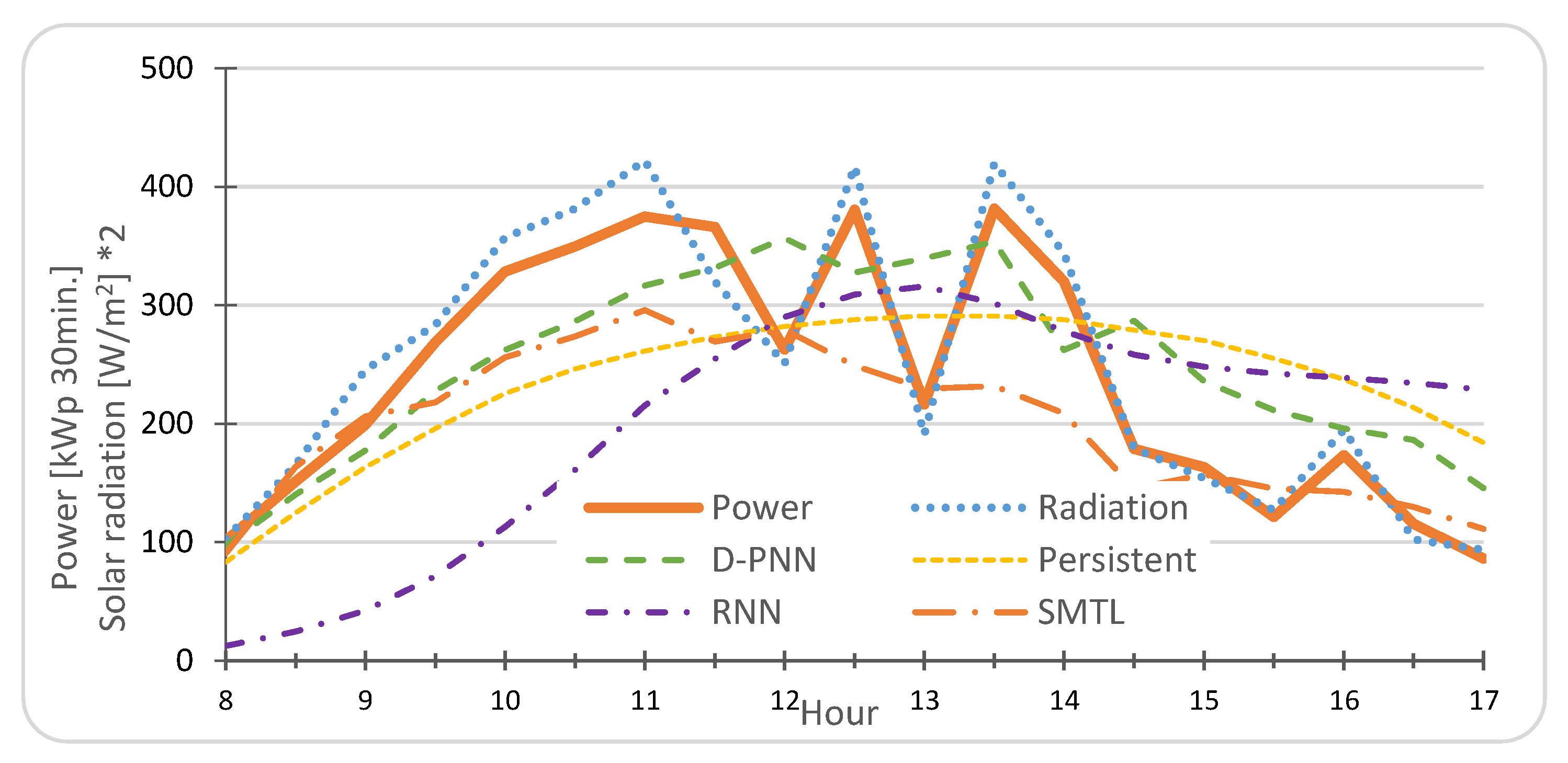
Figure 6 and Figure 7 demonstrate the intra-day 1–9 h and all-day 24 h prediction accuracy of both the approaches in characteristic days of the 14-day period of interest.
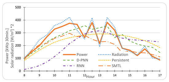
Figure 6.
St. Lhota, 17 May 2011—1–9 h prediction (most clear). RMSE: D-PNN = 65.0, persist. = 84.9, RNN = 125.3, SMLT = 67.1 kWp 30 min.

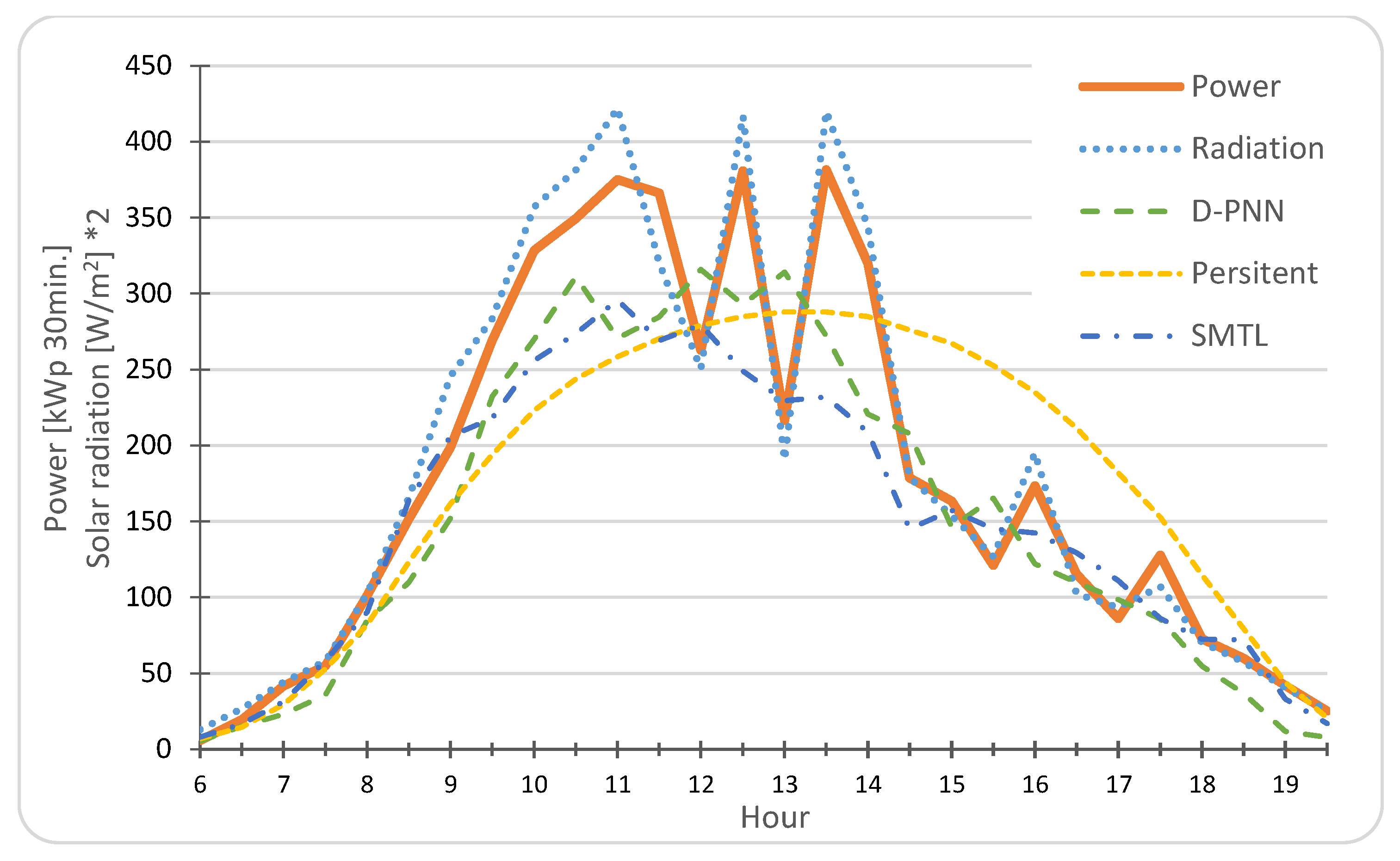
Figure 7.
St. Lhota, 17 May 2011—all-day prediction (variable cloudiness). MAE: D-PNN = 56.0, Persist. = 56.9, SMLT = 37.6 kWp 30 min.
6. 1–9 h and All-Day CSI/PVP Forecasting—Experiments Evaluation
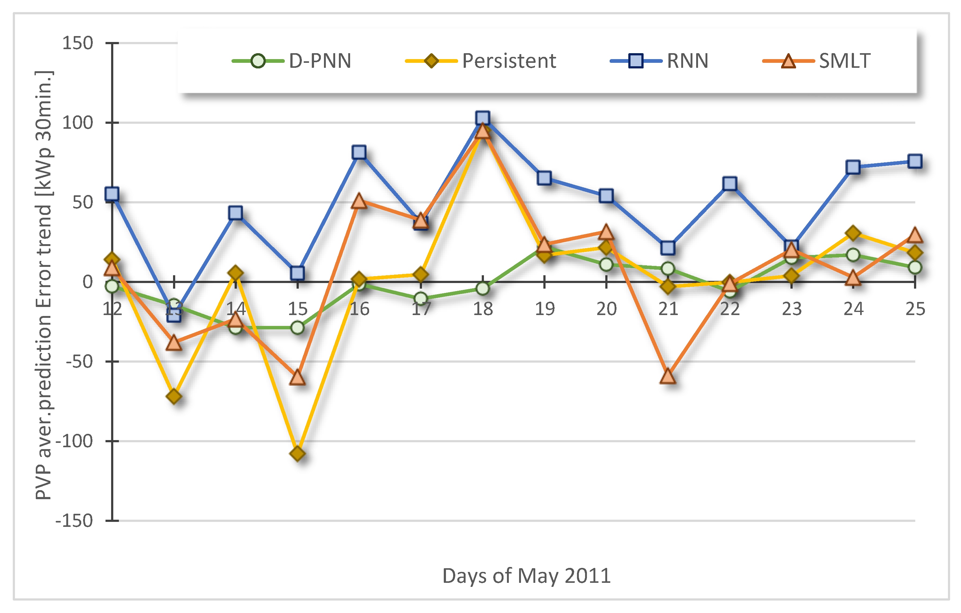
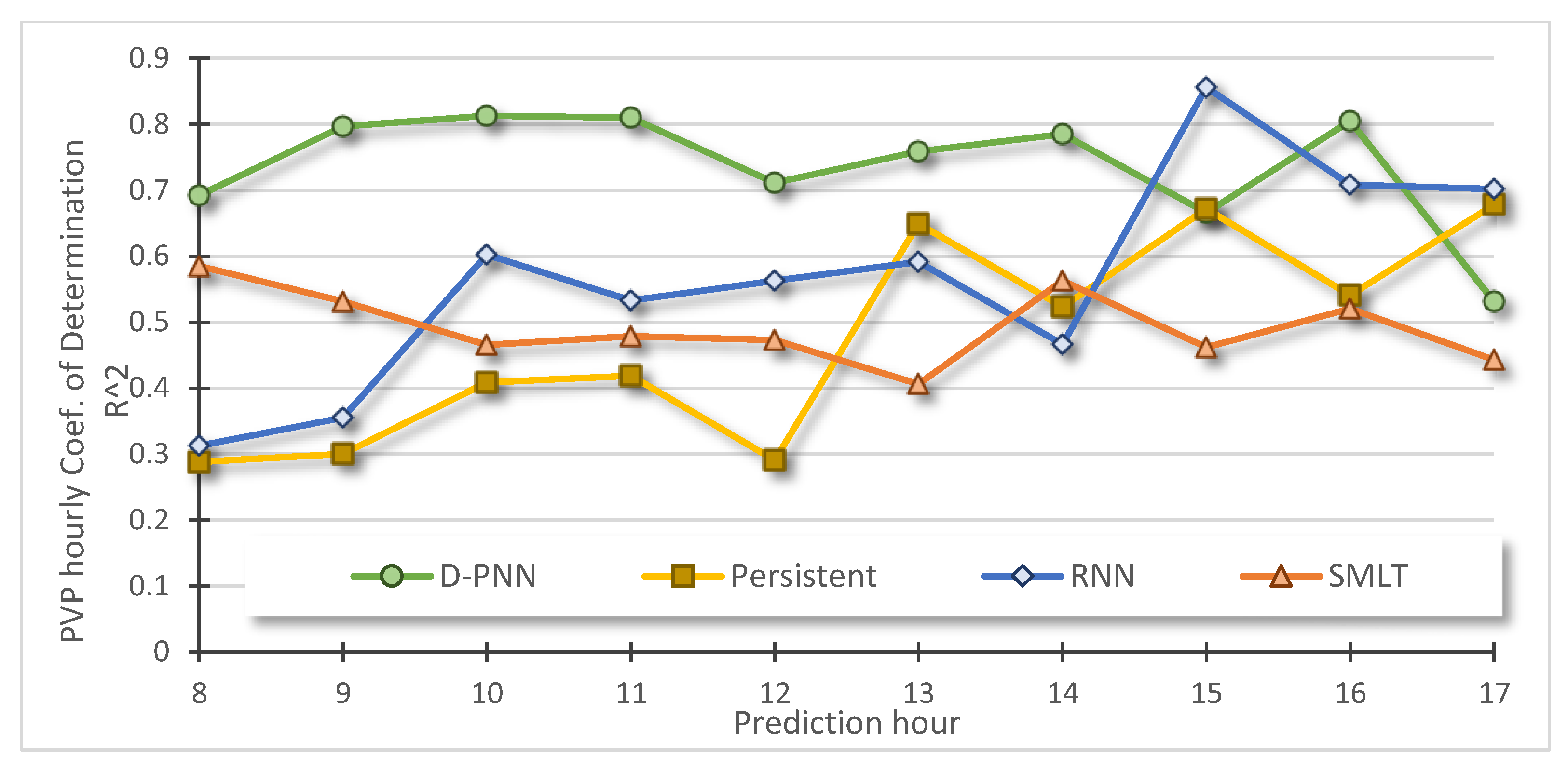
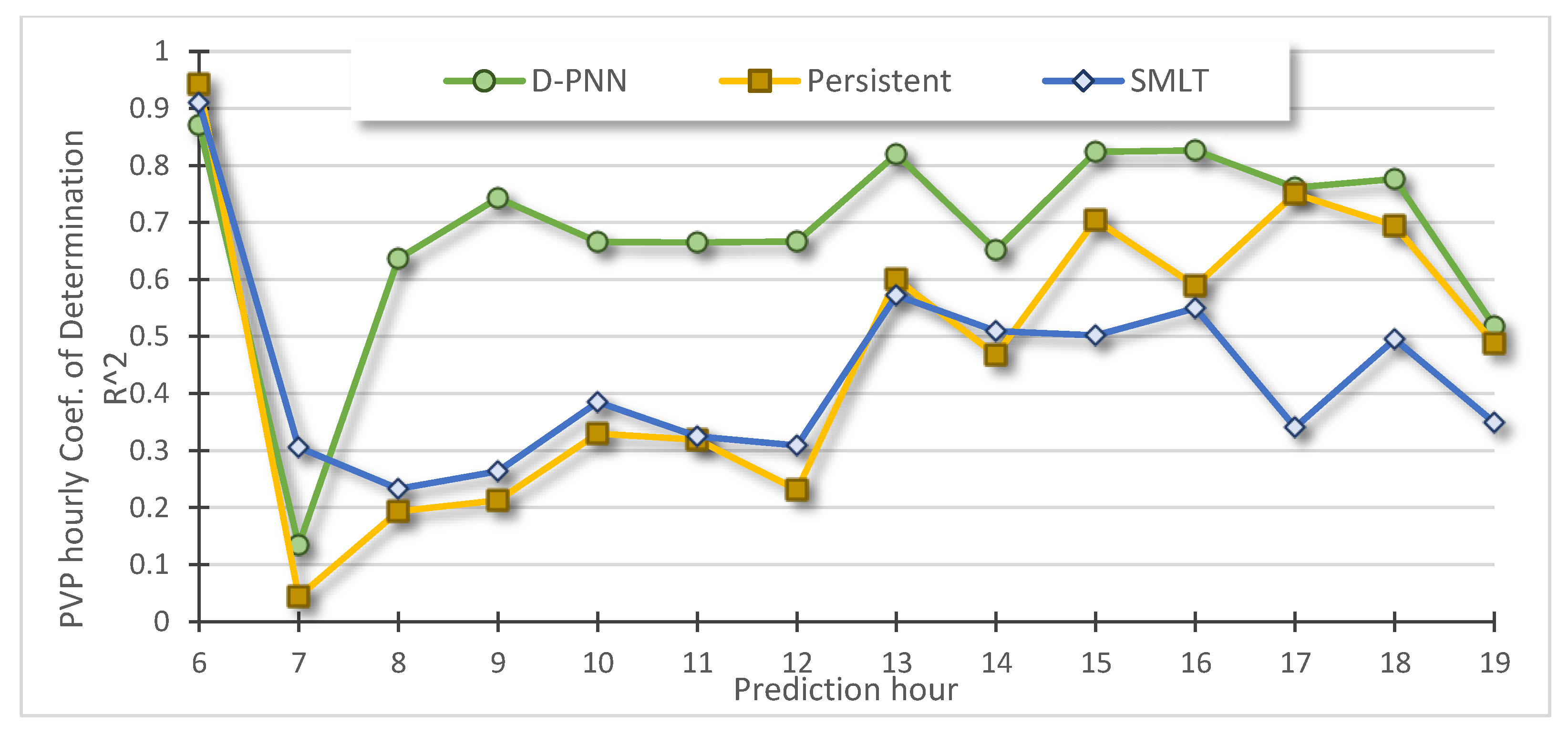
Figure 8 and Figure 9 present positive or negative trends in the daily average PVP prediction errors of the 1–9 h and all-day models, calculated in the intervals of hours at 8 a.m.–5 p.m. and 6 a.m.–7 p.m., respectively, in 14 days in a spring season, from 12 to 25 May 2011. The average 14-day PVP error trends are mostly balanced (around zero) in all the AI methods, except RNN processing calculated CSI in sequence in the nest time-step prediction and a slightly positive bias of the SMLT models. Pearson’s determination coefficient R2 was calculated for each prediction hour to assess the precision of statistical AI and persistent models in the predicted 1–9 and 24 h throughout the days (Figure 10 and Figure 11). The most stable output estimates without deflecting from the real PVP are produced by the D-PNN models.
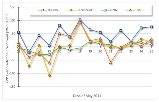
Figure 8.
14-day PVP intra-day 1–9 h average prediction error trends [kWp 30 min.]: D-PNN = −1.03, persist. = 2.10, RNN = 48.28, SMLT = 8.65.
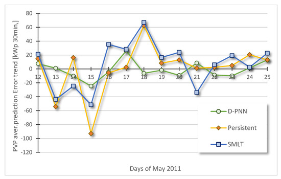
Figure 9.
14-day PVP all-day 24 h average prediction error trends [kWp 30 min.]: D-PNN = −1.19, persist. = 0.45, SMLT = 6.33.
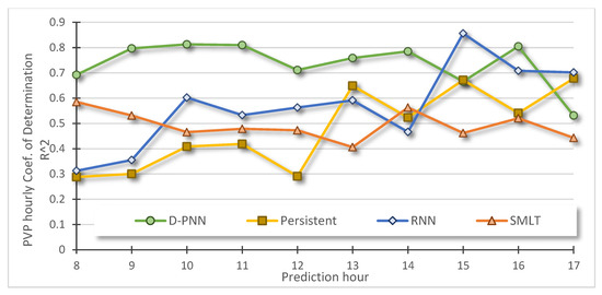
Figure 10.
14-day hourly PVP 1–9 h average prediction R2: D-PNN = 0.74, persist. = 0.48, RNN = 0.57, SMLT = 0.49 (8 a.m.–5 p.m.).
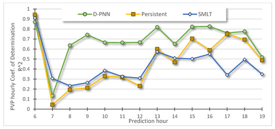
Figure 11.
14-day hourly PVP 24 h daily average prediction R2: D-PNN = 0.68, persist. = 0.47, SMLT = 0.43 (6 a.m.–7 p.m.).
Normalized errors allow us to express normalized nMAE (Mean Absolute Error) and nRMSE (Root Mean Squared Error) regardless of the peak values in predicted daily PVP cycles [3]. Table 2 and Table 3 summarize the nMAE and nRMSE of all the AI and statistical techniques presented in both the applied intraday and all-day prediction approaches. Low PVP production in the early morning and late evening times leads to the essential decrease in errors of the all-day 24 h models (Figure 7). The 1–9 h PVP models, which are not applicable to these edge data, are slightly disadvantaged in the accuracy assessment as a result of higher prediction PVP values and absolute errors calculated on the constrained time interval 8 a.m.–5 p.m. To make an adequate comparison of both the approaches, the errors of all-day models were calculated in the reduced interval hours to match the intra-day prediction data.
Table 2.
14-day PVP intra-day 8 a.m.–5 p.m. average—nRMSE, nMAE and R2, 12–25 May 2011.
Table 3.
14-day PVP daily 24 h 8 a.m.–5 p.m. average prediction—nRMSE, nMAE and R2, 12–25 May 2011.
RNN models usually represent an over-simplified daily PVP course; they can only sparsely predict its specific progress (Figure 7). Their deviations are already intense in predicting the closest morning hours (Figure 6), using prediction horizons in only a few hours. Persistent benchmarks can rarely obtain the better accuracy on days of changeable weather with unpredictable patterns, where the averaging of single CSI series properly compensates for the PVP uncertainty. These plain models can also better predict smooth daily PVP curves with no ramps in stable clear-sky conditions. Sophisticated AI methods that use more complex representations of data patterns may fail to identify longer training periods.
7. Discussion
The presented all-day prediction models can sometimes obtain better prediction accuracy than those making use of the intra-day forecasting scheme despite the higher 24 h time-horizon (Figure 10 and Figure 11). Rapid changes in the characteristics of weather patterns result in a great variability of data relations and practicability in training and prediction. The model quality usually varies according to the trained inputs–output time delay, applied in prediction, which is primarily related to the local near-ground dynamics and air flow. Regional NWP systems that use the earlier initialization time, that is, a higher prediction time, can analogously more precisely take into account local uncertainties, resulting in better compensation for anomalies in some aspects [2]. The accurate approximation of daily PVP progress mostly corresponds to stable periods of similar environmental conditions. Highly uncertain and variable patterns with PVP ramping in a short-time (Figure 7) lead to prediction difficulties and failures. Solar irradiation variances are usually higher after midday as a result of increased temperature with more intense air circulation. These phenomena usually lower the accuracy of PVP predictions of statistical models after noon [25].
Dissimilarities between historical and NWP data can be analyzed in augmented periods of several months to extract the optimal training samples, one by one, which primarily determine the usability of AI prediction models (Figure 11). Past overnight changes in weather can be searched first in order to detect the following interval of data records applicable in training. Additional input data with another 24 h delay of the entire day can improve the performance of AI models in specific periods of pattern (dis)similarity in some of the previous days to predict daily PVP cyclic data, analogous to relative humidity or power load [26].
In objectionable days following frontal changeovers, statistical all-day models using the 24 h prediction horizon are mainly all-over flawed (15 May, Figure 5). The prediction data patterns are absolutely different from those in the last days. A fixed testing error can be determined, according to the past failure cases with relation to NWP data, to assess the optimal model. If a test threshold or comparative limit is exceeded, the intra-day model, using the latest input data to calculate PVP in horizon of a few hours, can be re-evaluated in consideration of NWP. Failing the statistical test or comparative analysis, the AI-corrected or transformed forecast of the local NWP cloud amount (Weather underground historical data series: www.wunderground.com/history/daily/cz/mošnov/LKMT (accessed on 21 October 2021)) can be used [6]. No data preprocessing, component separation or additional transformation procedures were applied as mostly performed in the published strategies.
8. Conclusions
Two statistical approaches, using the fixed or gradually increased prediction horizon, were compared and evaluated with AI. The all-day procedure benefits from its low computational cost, forming one model all at once to predict complete PVP cycles in a day sequence. It obtains an adequate operational quality comparable to the intra-day results in the majority of days. Day-ahead models allow for timely planning of energy consumption in preparing effective load scenarios in the late evening before the plant operation day. The coming frontal waves change the current situation and stop the expected PVP production. New patterns are not or only little contained in historical sets of monthly data which do not allow their efficient learning. Intra-day models using the latest observations in predicting several hours ahead can be used in the sporadic day breaks in weather to eliminate the training limitations, testing failures and input over-delay causing shortcomings of 24 h models. D-PNN forms sets of simple PDEs that are solved using OC. Its summary PDE models, using selected daily data variables, can adequately represent the surface layer dynamics in local atmospheric processes. D-PNN outperforms stochastic soft-computing, or regression unable to reliably model complex weather patterns and their variability to meet PVP plant operational specifications. Its PDE-components are dynamically formed to be included in the composite model which is more robust and resistant to chaotic fluctuations and uncertainties in local weather. In addition, they do not require exact recognition of the optimal training samples. D-PNN predicts daily PVP progress and peak maxima with acceptable accuracy, especially on days of unstable weather conditions, responding to rapid development and changes in cloud structures. Parametric C++ application software of D-PNN with the applied power data is available to allow reproducibility of the prediction results (D-PNN application C++ parametric software and Power data: https://drive.google.com/drive/folders/1ZAw8KcvDEDM-i7ifVe_hDoS35nI64-Fh?usp=sharing (accessed on 21 October 2021)).
Funding
SGS project: VŠB-Technical University of Ostrava, Czech Republic, under the grant No. SP2021/24 “Parallel processing of Big Data VIII”.
Institutional Review Board Statement
Not applicable.
Informed Consent Statement
Not applicable.
Data Availability Statement
D-PNN application C++ parametric software and Power data are available for free.
Acknowledgments
This work was supported by SGS, VŠB-Technical University of Ostrava, Czech Republic, under the grant No. SP2021/24 “Parallel processing of Big Data VIII”.
Conflicts of Interest
The authors declare no conflict of interest.
References
- Sobri, S.; Koohi-Kamali, S.; Rahim, N.A. Solar photovoltaic generation forecasting methods: A review. Energy Convers. Manag. 2018, 156, 459–497. [Google Scholar] [CrossRef]
- Vannitsem, S. Dynamical Properties of MOS Forecasts: Analysis of the ECMWF Operational Forecasting System. Weather Forecast. 2008, 23, 1032–1043. [Google Scholar] [CrossRef]
- Giorgi, M.G.D.; Congedo, P.M.; Malvoni, M.; Laforgia, D. Error analysis of hybrid photovoltaic power forecasting models: A case study of mediterranean climate. Energy Convers. Manag. 2015, 100, 117–130. [Google Scholar] [CrossRef]
- Leva, S.; Dolara, A.; Grimaccia, F.; Mussetta, M.; Ogliari, E. Analysis and validation of 24 hours ahead neural network forecasting of photovoltaic output power. Math. Comput. Simul. 2017, 131, 88–100. [Google Scholar] [CrossRef] [Green Version]
- Shamim, M.A.; Remesan, R.; Bray, M.; Han, D. An improved technique for global solar radiation estimation using numerical weather prediction. J. Atmos. Sol.-Terr. Phys. 2015, 129, 13–22. [Google Scholar] [CrossRef]
- Zjavka, L.; Krömer, P.; Mišák, S.; Snášel, V. Modeling the Photovoltaic Output Power using the Differential Polynomial Network and Evolutional Fuzzy Rules. Math. Model. Anal. 2017, 22, 78–94. [Google Scholar] [CrossRef] [Green Version]
- Wan, C.; Zhao, J.; Song, Y.; Xu, Z.; Lin, J.; Hu, Z. Photovoltaic and Solar Power Forecasting for Smart Grid Energy Management. CSEE J. Power Eenergy Syst. 2015, 1, 38–46. [Google Scholar] [CrossRef]
- Nikolaev, N.Y.; Iba, H. Adaptive Learning of Polynomial Networks. Genetic and Evolutionary Computation; Springer: New York, NY, USA, 2006. [Google Scholar]
- Akhter, M.N.; Mekhilef, S.; Mokhlis, H.; Shah, N.M. Review on forecasting of photovoltaic power generation based on machine learning and metaheuristic techniques. IET Renew. Power Gener. 2019, 13, 1009–1023. [Google Scholar] [CrossRef] [Green Version]
- Agoua, X.G.; Girard, R.; Kariniotakis, G. Photovoltaic Power Forecasting: Assessment of the Impact of Multiple Sources of Spatio-Temporal Data on Forecast Accuracy. Energies 2021, 14, 1432. [Google Scholar] [CrossRef]
- Rana, M.; Rahman, A. Multiple steps ahead solar photovoltaic power forecasting based on univariate machine learning models and data re-sampling. Sustain. Energy Grids Netw. 2020, 21, 100286. [Google Scholar] [CrossRef]
- Liu, Z.F.; Luo, S.F.; Tseng, M.L.; Liu, H.M.; Li, L. Short-term photovoltaic power prediction on modal reconstruction: A novel hybrid model approach. Sustain. Energy Technol. Assess. 2021, 45, 101048. [Google Scholar] [CrossRef]
- Das, U.K.; Teya, K.S.; Seyedmahmoudiana, M.; Mekhilef, S. Forecasting of photovoltaic power generation and model optimization: A review. Renew. Sustain. Energy Rev. 2018, 81, 912–928. [Google Scholar] [CrossRef]
- Yin, W.; Han, Y.; Zhou, H.; Ma, M.; Li, L.; Zhu, H. A novel non-iterative correction method for short-term photovoltaic power forecasting. Renew. Energy 2020, 159, 23–32. [Google Scholar] [CrossRef]
- Dewangan, C.L.; Singh, S.N.; Chakrabarti, S. Combining forecasts of day-ahead solar power. Energy 2020, 202, 117743. [Google Scholar] [CrossRef]
- Wang, K.; Qi, X.; Liu, H. Photovoltaic power forecasting based LSTM-Convolutional Network. Energy 2019, 189, 116225. [Google Scholar] [CrossRef]
- Gao, M.; Li, J.; Hong, F.; Long, D. Day-ahead power forecasting in a large-scale photovoltaic plant based on weather classification using LSTM. Energy 2019, 187, 115838. [Google Scholar] [CrossRef]
- Mayer, M.J.; Grof, G. Extensive comparison of physical models for photovoltaic power forecasting. Appl. Energy 2021, 187, 116239. [Google Scholar] [CrossRef]
- Lin, P.; Peng, Z.; Lai, Y.; Cheng, S.; Chen, Z.; Wu, L. Short-term power prediction for photovoltaic power plants using a hybrid improved Kmeans-GRA-Elman model based on multivariate meteorological factors and historical power datasets. Energy Convers. Manag. 2018, 177, 704–717. [Google Scholar] [CrossRef]
- Mouna Diagne, H.M.; David, M.; Lauret, P.; Boland, J.; Schmutz, N. Review of solar irradiance forecasting methods and a proposition for small-scale insular grids. Renew. Sustain. Energy Rev. 2013, 27, 65–76. [Google Scholar] [CrossRef] [Green Version]
- Pelland, S.; Remund, J.; Kleissl, J.; Oozeki, T.; Brabandere, K.D. Photovoltaic and Solar Forecasting: State of the Art. Photovoltaic Power Systems Programme; IEA International Energy Agency: Paris, France, 2013. [Google Scholar]
- Giorgi, M.G.D.; Malvoni, M.; Congedo, P.M. Comparison of strategies for multi-step ahead photovoltaic power forecasting models based on hybrid group method of data handling networks and least square support vector machine. Energy 2016, 107, 360–373. [Google Scholar] [CrossRef]
- Zjavka, L.; Pedrycz, W. Constructing General Partial Differential Equations using Polynomial and Neural Network. Neural Netw. 2016, 73, 58–69. [Google Scholar] [CrossRef] [PubMed]
- Anastasakis, L.; Mort, N. The Development of Self-Organization Techniques in Modelling: A Review of the Group Method of Data Handling (GMDH); The University of Sheffield: Sheffield, UK, 2001. [Google Scholar]
- Coimbra, C.; Kleissl, J.; Marquez, R. Overview of Solar Forecasting Methods and a Metric for Accuracy Evaluation; Elsevier: Amsterdam, The Netherlands, 2013; pp. 171–194. [Google Scholar]
- Zjavka, L.; Sokol, Z. Local Improvements in Numerical Forecasts of Relative Humidity Using Polynomial Solutions of General Differential Equations. Q. J. R. Meteorol. Soc. 2018, 144, 780–791. [Google Scholar] [CrossRef]


Publisher’s Note: MDPI stays neutral with regard to jurisdictional claims in published maps and institutional affiliations. |
© 2021 by the author. Licensee MDPI, Basel, Switzerland. This article is an open access article distributed under the terms and conditions of the Creative Commons Attribution (CC BY) license (https://creativecommons.org/licenses/by/4.0/).