Comparison of the Reactive Scalar Gradient Evolution between Homogeneous MILD Combustion and Premixed Turbulent Flames

Abstract

Moderate or intense low-oxygen dilution (MILD) combustion is a novel combustion technique that can simultaneously improve thermal efficiency and reduce emissions. This paper focuses on the differences in statistical behaviours of the surface density function (SDF = magnitude of the reaction progress variable gradient) between conventional premixed flames and exhaust gas recirculation (EGR) type homogeneous-mixture combustion under MILD conditions using direct numerical simulations (DNS) data. The mean values of the SDF in the MILD combustion cases were found to be significantly smaller than those in the corresponding premixed flame cases. Moreover, the mean behaviour of the SDF in response to the variations of turbulence intensity were compared between MILD and premixed flame cases, and the differences are explained in terms of the strain rates induced by fluid motion and the ones arising from flame displacement speed. It was found that the effects of dilatation rate were much weaker in the MILD combustion cases than in the premixed flame cases, and the reactive scalar gradient in MILD combustion cases preferentially aligns with the most compressive principal strain-rate eigendirection. By contrast, the reactive scalar gradient preferentially aligned with the most extensive principal strain-rate eigendirection within the flame in the premixed flame cases considered here, but the extent of this alignment weakened with increasing turbulence intensity. This gave rise to a predominantly positive mean value of normal strain rate in the premixed flames, whereas the mean normal strain rate remained negative, and its magnitude increased with increasing turbulence intensity in the MILD combustion cases. The mean value of the reaction component of displacement speed assumed non-negligible values in the MILD combustion cases for a broader range of reaction progress variable, compared with the conventional premixed flames. Moreover, the mean displacement speed increased from the unburned gas side to the burned gas side in the conventional premixed flames, whereas the mean displacement speed in MILD combustion cases decreased from the unburned gas side to the middle of the flame before increasing mildly towards the burned gas side. These differences in the mean displacement speed gave rise to significant differences in the mean behaviour of the normal strain rate induced by the flame propagation and effective strain rate, which explains the differences in the SDF evolution and its response to the variation of turbulence intensity between the conventional premixed flames and MILD combustion cases. The tangential fluid-dynamic strain rate assumed positive mean values, but it was overcome by negative mean values of curvature stretch rate to yield negative mean values of stretch rate for both the premixed flames and MILD combustion cases. This behaviour is explained in terms of the curvature dependence of displacement speed. These findings suggest that the curvature dependence of displacement speed and the scalar gradient alignment with local principal strain rate eigendirections need to be addressed for modelling EGR-type homogeneous-mixture MILD combustion.

1. Introduction

Fossil fuels are expected to supply 85% of the primary energy required for transportation until 2040 [1]. Thus, these fuels will continue to be a major energy source for applications involving high energy density, such as in the transport sector [1], at least for a foreseeable future. Fossil fuel combustion is a major contributor to pollutants and greenhouse gas emissions. Thus, it is imperative for the new generation of combustion devices to be both energy-efficient and environmentally friendly. Moderate or intense low-oxygen dilution (MILD) combustion is one of the modern concepts with the potential to deliver both high-energy efficiency and ultra-low emission [2,3,4]. This concept involves a fuel-air mixture preheated above its autoignition temperature [4], which can be achieved by recirculating the hot flue gas of furnaces and boilers [5]. Such gas recirculation inherently increases the thermal efficiency of furnaces and boilers, as the maximum temperature rise remains smaller than the autoignition temperature [4,5]. MILD combustion provides uniform temperature distribution, extremely low levels of NOx, CO and greenhouse gases, high thermal efficiency, and excellent combustion stability. All of these make this technique attractive for power generation and process applications. MILD combustion is characterised by (a) high level of dilution by burnt gases such that the temperature rise $∆T$ remains smaller than the autoignition temperature $T_{\mathrm{ign}}$ (i.e., $∆T<T_{\mathrm{ign}}$), and (b) the reactants are significantly preheated such that the reactant temperature $T_0$ remains greater than $T_{\mathrm{ign}}$ (i.e., $T_0>T_{\mathrm{ign}}$) [4]. This definition of MILD combustion (alternatively known as flameless combustion) follows from the well-stirred reactor (WSR) theory, which can be readily applied to turbulent premixed combustion. MILD combustion has been analysed extensively [4,5,6,7,8,9,10,11,12,13,14,15] by experimental means to understand the underlying combustion process. Plessing et al. [6] compared MILD combustion with conventional combustion by investigating both planar laser-induced fluorescence images of OH radicals (OH-PLIF) and Rayleigh thermometry. The presence of flame fronts in MILD combustion was observed using OH-PLIF but the temperature measurements revealed indications of distributed burning. A similar observation was also reported by Ozdemir and Peters [10] based on their experimental investigations. Several Reynolds averaged Navier–Stokes (RANS) and large eddy simulations (LES) investigations of MILD combustion using conventional flamelet and eddy dissipation approaches [8,9,13,16,17] have also been conducted which reported good agreement with experimental data in terms of mean velocity and temperature fields, but discrepancies have been reported in terms of peak temperature and minor species (e.g., CO and OH) concentrations [8,12]. The advancements in high-performance computing have enabled direct numerical simulations (DNS) of MILD combustion [18,19,20,21,22,23,24,25,26,27]. Van Oijen [18] carried out DNS of autoigniting mixing layers of CH₄/H₂ fuel-blends and provided important insights to the roles of non-unity Lewis number and O₂ dilution on autoignition delay under MILD combustion conditions. Minamoto, Swaminathan and co-workers [18,19,20,21,22] analysed the distribution of species, temperature, and reaction-rate fields [18,19], morphological and topological structures [20] and scalar gradient statistics in terms of temperature and equivalent OH-PLIF signal [21] constructed from DNS data based on three-dimensional simulations of the combustion an exhaust gas recirculation (EGR)-type homogeneous-mixture under MILD conditions. They concluded that the appearance of a distributed combustion is due to the interaction of thin reaction zones [19,20,21,22,23], which were also reported based on OH-PLIF visualisations [4,10,14,15]. These analyses have been further extended by Doan, Swaminathan and co-workers for stratified-mixture MILD combustion [24,25,26] and provided important insights into the flame structure [24,25], reaction-zone topology [24,25] and markers of combustion mode [26]. A review of the physical insights gained from DNS can be found in [27]. These DNS analyses [19,20,21,22,23,24,25,26] revealed that the convolution of the reaction zones in MILD combustion is not only affected by turbulence–chemistry interaction but the dilution factor also plays a significant role. Furthermore, recent studies [20,23] using DNS data have indicated that flamelet-based models can be applied to gaseous-fuel MILD combustion with some modifications, which is contrary to the conventional expectation that flamelet closures are unlikely to be valid for distributed reactions expected in MILD conditions. As flamelet models need the statistics of the reactive scalar gradient, it is important to investigate the statistical behaviour of the gradient of the reaction progress variable, $c$ (surface density function (SDF) =|$\nabla c$| [28]), since it is closely related to the scalar dissipation rate (SDR) $N_c=D_c{\left| \nabla c\right|}^2$ (with $D_c$ being the reaction progress variable diffusivity) [29,30] and generalised flame surface density (FSD) (${\mathsf{\Sigma }}_{\mathrm{gen}}=\left|\overline{\nabla c}\right|$ with the overbar, suggesting a Reynolds averaging/LES filtering operation, as appropriate) [31], which are often used for the modelling of the combustion of homogeneous-mixtures. In this respect, it is important to understand the influence of the strain rates induced by fluid motion and flame propagation on SDF evolution in homogeneous-mixture MILD combustion, and the differences in these mechanisms in comparison with conventional premixed combustion. Although the SDF evolution within the flame front and the strain rates affecting this process have been extensively analysed, in the case of conventional premixed flames [28,32,33,34,35,36,37,38,39,40,41,42,43,44], this aspect has rarely been addressed in the case of EGR-type homogeneous-mixture MILD combustion [23]. The present analysis aims to address this gap in the existing literature by conducting three-dimensional DNS with a skeletal methane–air chemical mechanism [45] for EGR-type homogeneous-mixture combustion under MILD conditions, in the case of an O₂ dilution percentage of 4.8% by volume, for an equivalence ratio of $\varphi =0.8$ under different root–mean–square turbulent-velocity fluctuations $u^{\prime }$. The SDF statistics of these MILD combustion cases have been compared to the corresponding statistics obtained from DNS of undiluted CH4–air premixed flames of $\varphi =0.8$ with an unburned gas temperature of $T_0=300 \mathrm{K}$ following the methodology adopted previously by Minamoto, Swaminathan and co-workers [19,20,21,22,23] to compare the flame statistics between EGR-type homogeneous-mixture MILD combustion and conventional premixed combustion. In this respect, the main objectives of the current analysis are:

• A comparison between the SDF statistics in EGR-type homogeneous-mixture MILD combustion and conventional premixed combustion to understand how different strain rates influence the SDF evolution in MILD combustion under different turbulence intensities.
• Modelling implication of the differences in the SDF statistics between MILD and conventional premixed turbulent combustion.

The rest of the paper will be organised as follows. The mathematical background pertaining to this analysis will be presented in the next section. This will be followed by a brief discussion of the numerical implementation. Following that, the results will be presented and subsequently discussed. Finally, key findings will be summarised, and conclusions will be drawn.

2. Mathematical Background

The extent of the completion of the chemical reaction can be quantified in terms of a reaction progress variable $c$, which increases monotonically from 0.0, in the unburned gas, to 1.0 in the fully burned products. For the present analysis, the reaction progress variable $c$ is defined based on the fuel mass fraction $Y_F$ (i.e., CH₄ mass fraction) in the following manner:

$$c=\frac{Y_{\mathit{FR}}-Y_F}{Y_{\mathit{FR}}-Y_{\mathit{FP}}}$$

(1)

where subscripts R and P refer to values in unburned reactants and fully burned products. The reaction progress variable transport is governed by [46]:

$$\rho \frac{\partial c}{\partial t}+{\rho u}_j\frac{\partial c}{\partial x_j}=\frac{\partial }{\partial x_j}\left({\rho D}_c\frac{\partial c}{\partial x_j}\right)+{ \dot{\omega } }_c$$

(2)

where, $\rho$ is the gas density,$D_c$ is the mass diffusivity of the species based on which the reaction progress variable is defined, $u_j$ is the $j^{\mathrm{th}}$ velocity component, and ${\dot{\omega }}_c$ is the reaction rate of the reaction progress variable. The reaction rate of the progress variable ${\dot{\omega }}_c$ is expressed as follows [46]:

$${ \dot{\omega }}_c=-{\dot{\omega }}_F/\left(Y_{\mathit{FR}}-Y_{\mathit{FP}}\right)$$

(3)

where ${\dot{\omega }}_F$ is the fuel reaction rate. Equation (2) can be rewritten for a given $c$ iso-surface in the following manner [46]:

$$\left(\partial c/\partial t+u_j\partial c/\partial x_j\right)=S_d\left|\nabla c\right|$$

(4)

where$S_d$is the displacement speed at a given c iso-surface and it is given by:

$$S_d=[{\dot{\omega }}_c+\nabla ·\left(\rho D\nabla c\right)]/\rho \left|\nabla c\right|$$

(5)

The displacement speed arises because of the relative balance between its components, and can be split in the following manner [46,47,48]:

$$S_d=S_r+S_n+S_t$$

(6)

Here, $S_r, S_n$ and$S_t$ are the reaction, normal diffusion and tangential diffusion components of displacement speed, respectively, which are defined as [48,49,50]:

$$S_r=\frac{\dot{{\omega }_c}}{\rho \left|\nabla c\right|}; S_n=\frac{\overrightarrow{N}·\nabla (\rho D\overrightarrow{N}·\nabla c)}{\rho \left|\nabla c\right|};S_t=-2D{\kappa }_m$$

(7)

where, $\overrightarrow{N}=-\nabla c/\left|\nabla c\right|$ is the flame-normal vector and ${\kappa }_m=0.5\nabla ·\overrightarrow{N}$ is the mean flame curvature. According to these definitions, the flame-normal points towards the unburned gas and a reaction progress variable iso-surface has a positive (negative) curvature when it is convexly (concavely) curved towards the reactants.

The transport equation for the magnitude of the reaction progress variable gradient (i.e., surface density function (SDF) [28]) for a given $c$-isosurface takes the following form [31,32,33,34,35,36,37,38,39,40,41,42,43,44]:

$$\frac{\partial \left|\nabla c\right|}{\partial t}+\frac{\partial \left(u_j\left|\nabla c\right|\right)}{\partial x_j}=a_T\left|\nabla c\right|-\frac{\partial \left(S_d{N}_j\left|\nabla c\right|\right)}{\partial x_j}+2S_d{\mathsf{\kappa }}_m\left|\nabla c\right|$$

(8)

where, $a_T\left|\nabla c\right|$ is the SDF strain rate term with $a_T=\left({\delta }_{ij}-N_i{N}_j\right)\partial u_i/\partial x_j$ being the tangential strain rate, $-\partial \left(S_d{N}_j\left|\nabla c\right|\right)/\partial x_j$ arises due to flame-normal propagation and thus referred to as the SDF propagation term, $2S_d{\kappa }_m\left|\nabla c\right|$ originates due to curvature and therefore is referred to as the SDF curvature term. Equation (8) can be rewritten as [37,38,39]:

$$\frac{1}{\left|\nabla c\right|}\frac{d\left|\nabla c\right|}{dt}=-\frac{1}{∆x_N}\frac{d∆x_N}{dt}=-a_N-N_j\frac{\partial S_d}{\partial x_j}=-a_N^{\mathit{eff}}$$

(9)

where, $d(\dots )/dt=\partial (\dots )/\partial t+V_j^c\partial (\dots )/\partial x_j$ is the total derivative in the reference frame attached to the flame, $V_j^c=u_j+S_d{N}_j$ is the jth component of flame propagation velocity, $∆x_N$ is the distance between two adjacent $c$-isosurfaces, $a_N=N_i{N}_j\partial u_i/\partial x_j$ is the fluid-dynamic normal strain rate, $N_j\partial S_d/\partial x_j$ is the normal strain rate induced by flame propagation and $a_N^{eff}=a_N+N_j\partial S_d/\partial x_j$ is the effective normal strain rate [37,38,39]. It is evident from Equation (9) that a positive value of $a_N^{eff}$ acts to increase the distance between two adjacent $c$-isosurfaces, which in turn decreases $\left|\nabla c\right|$. By contrast, a negative value of $a_N^{eff}$ decreases the distance between two adjacent $c$-isosurfaces, and therefore increases $\left|\nabla c\right|$.

As $\left|\nabla c\right|$ is closely related to the surface area of the reaction zone, it is worthwhile to consider the evolution of the elemental reaction zone surface area $\delta A$ [37,38,39,49,50]:

$$\frac{1}{\delta A}\frac{d\left(\delta A\right)}{dt}=a_T+2S_d{\mathsf{\kappa }}_m=a_T^{\mathit{eff}}$$

(10)

Here, $a_T^{eff}$ is commonly referred to as the flame stretch rate or the effective tangential strain rate, where $a_T$ is the flow component of $a_T^{eff}$ and the component $2S_d{\kappa }_m$ arises due to flame propagation and therefore is commonly termed as the curvature stretch rate.

It is evident from the above discussion that $a_N,a_T,N_j\partial S_d/\partial x_j,2S_d{\kappa }_m,a_N^{eff}$ and $a_T^{eff}$ determine the evolutions of the SDF and the area of the reaction zone and thus the statistical behaviours of these strain rates will be discussed in detail in Section 4 of this paper.

3. Numerical Implementation

A compressible DNS code SENGA2 [51] is used for the simulations conducted in the current study. In SENGA2, the standard conservation equations of mass, momentum, energy and species mass fractions for compressible reacting flows are solved in dimensional form. The thermophysical properties, such as viscosity, thermal conductivity, specific heat capacities and mass diffusivities, are taken to be temperature-dependent and are expressed in terms of polynomials similar in form to CHEMKIN polynomials [51]. A 10th-order central difference scheme is used for spatial differentiation at the internal grid points, but the order of accuracy gradually reduces to a one-sided fourth-order scheme at the non-periodic boundaries. A fourth-order explicit low-storage Runge–Kutta scheme is used for time advancement. The boundary conditions are specified according to the Naiver–Stokes characteristic boundary condition (NSCBC) methodology [52]. A skeletal chemical mechanism comprising 16 species and 25 reactions (including 10 reversible reactions) has been taken to represent the chemical kinetics of ${\mathrm{CH}}_4/$ Air combustion [45]. A domain, of size $10 \mathrm{mm}\times 10 \mathrm{mm}\times 10 \mathrm{mm}$ and discretized by a Cartesian grid of $252\times 252\times 252$ with uniform grid spacing, has been used for the simulations of MILD CH₄-air mixtures with an O₂ dilution percentage of 4.8% by volume for an equivalence ratio of $\varphi =0.8$ and an initial temperature of about 1500 K (i.e., $T_0\approx 1500 \mathrm{K}$). The unburned gas temperature of 1500 K is higher than the autoignition temperature (i.e., $T_{\mathrm{ign}}=1100 \mathrm{K}$ based on well-stirred reactor calculations [19,20,21,22,23]) for CH₄-air mixtures with an O₂ dilution percentage of 4.8% by volume for an equivalence ratio of $\varphi =0.8$. The simulation domain consists of a turbulent inflow with specified density, velocity and species at the left-hand $x_1-$boundary and a partially non-reflective outflow boundary condition is specified at the right-hand $x_1-$ boundary. All other boundaries are taken to be periodic.

For the purpose of comparison, DNS calculations of statistically planar conventional turbulent premixed flames of $\varphi =0.8$ with an unburned gas temperature of 300 K have been conducted for a domain size of $20 \mathrm{mm}\times 10 \mathrm{mm}\times 10 \mathrm{mm}$, which was discretized by a uniform Cartesian grid of $504\times 252\times 252$. A longer domain in the streamwise flow direction was taken for the turbulent premixed flame simulations to allow for flame propagation in the mean direction of flame propagation (which is taken to align with the $x_1-$ direction) without the influence of computational boundaries. In the premixed flame simulations, the domain boundaries in the direction of the mean flame propagation were taken to be partially non-reflecting, and transverse boundaries were taken to be periodic.

The grid spacing for both the MILD and premixed combustion simulations ensures that the thermal flame thickness ${\delta }_{th}=\left(T_P-T_0\right)/max{\left|\nabla T\right|}_L$ (with $T, T_p$ and $T_0$ being the instantaneous, product and reactant temperatures, respectively and subscript L refers to the values in the corresponding 1D unstretched premixed flame) is resolved using at least 12 grid points. The grid spacing also ensured the resolution of the Kolmogorov length scale, $\eta$, by at least 1.5 grid points for all turbulent cases.

The thermochemical conditions in the unburned gas, including the mole fractions of the reactants, and unburned gas temperature for the MILD and the lean premixed cases are shown in

Table 1. Thermochemical conditions.

Case	${\mathit{X}}_{{\mathit{O}}_{\mathbf{2}}}$	${\mathit{X}}_{\mathit{C}{\mathit{O}}_{\mathbf{2}}}$	${\mathit{X}}_{{\mathit{H}}_{\mathbf{2}}\mathit{O}}$	${\mathit{X}}_{{\mathit{C}\mathit{H}}_{\mathbf{4}}}$	${\mathit{X}}_{{\mathit{N}}_{\mathbf{2}}}$	${\mathit{T}}_{\mathbf{0}}\mathbf{(}\mathit{K}\mathbf{)}$
MILD	0.048	0.061	0.121	0.019	0.751	1500
Premixed	0.194	0.0	0.0	0.077	0.729	300

. Under the conditions summarised in Table 1, the unstretched laminar burning velocity, $S_L$, is $3.20 \mathrm{m}/\mathrm{s}$ and $0.28 \mathrm{m}/\mathrm{s}$ for the MILD and the lean premixed cases, respectively, under atmospheric pressure. The simulations have been conducted for different initial values of turbulence intensities $u^{\prime }/S_L$ for a given normalised value of integral length scale of turbulence $l/{\delta }_{th}$ where $l$ is the integral length scale of turbulence. The initial values of $u^{\prime }/S_L$ and $l/{\delta }_{th}$ along with the values of Damköhler number $Da=l{S}_L/u^{\prime }{\delta }_{th}$ and Karlovitz number $Ka={\left(u^{\prime }/S_L\right)}^{3/2}{\left(l/{\delta }_{th}\right)}^{-1/2}$ are summarised in

Table 2. Initial Turbulence parameters.

Case	${\mathit{u}}^{\mathsf{\prime }}\mathsf{/}{\mathit{S}}_{\mathit{L}}$	$\mathit{l}\mathsf{/}{\mathsf{\delta }}_{\mathit{t}\mathit{h}}$	$\mathit{D}\mathit{a}$	$\mathit{K}\mathit{a}$
Premixed	4.0	2.5	0.62	5.06
	6.0	2.5	0.42	9.30
	8.0	2.5	0.31	14.31
MILD	4.0	2.5	0.62	5.06
	6.0	2.5	0.42	9.30
	8.0	2.5	0.31	14.31

. The turbulence levels reported in Table 2 matches and expands upon those used by Minamoto et al. [19,20,21,22] and represent a jet in hot co-flow (JHC)-type flame configuration. This provides a base line to validate the current DNS dataset against, while also expanding the investigation to include the effect of turbulence intensities on homogeneous MILD combustion. It is worth noting the identical values of $u^{\prime }/S_L$ and $l/{\delta }_{th}$ between the MILD and premixed cases ensure that they are nominally in the same location on the Borghi–Peters diagram [53] and all the cases considered here nominally represent combustion within the thin reaction zones regime [53]. It is important to note that the turbulent Reynolds number $R{e}_t=u^{\prime }l/\nu$ with $\nu$ being the kinematic viscosity scales as: $R{e}_t~\left(u^{\prime }/S_L\right)\left(l/{\delta }_{th}\right)$. Thus, the identical values of $u^{\prime }/S_L$ and $l/{\delta }_{th}$ between the MILD and premixed cases also ensure that they have comparable values of $R{e}_t$.

The MILD combustion simulations are split into two stages, which are summarised in Figure 1. The first stage corresponds to the mixing of the products of combustion with the reactant mixture. The second stage simulates the combustion process [19,20,21,22,23]. The species field obtained from the first stage acts as the initial, as well as the inflow fields for the second stage. The first stage mimics what happens inside the recirculation zone of a real MILD combustor. The mixture at stage 1 is prepared according to the following steps, as reported by Minamoto, Swaminathan and co-workers [19,20,21,22,23]:

• A homogenous isotropic field, generated using a well-known pseudo-spectral method [54], is used to initialize turbulent velocity fluctuations following the Batchelor–Townsend spectrum [55].
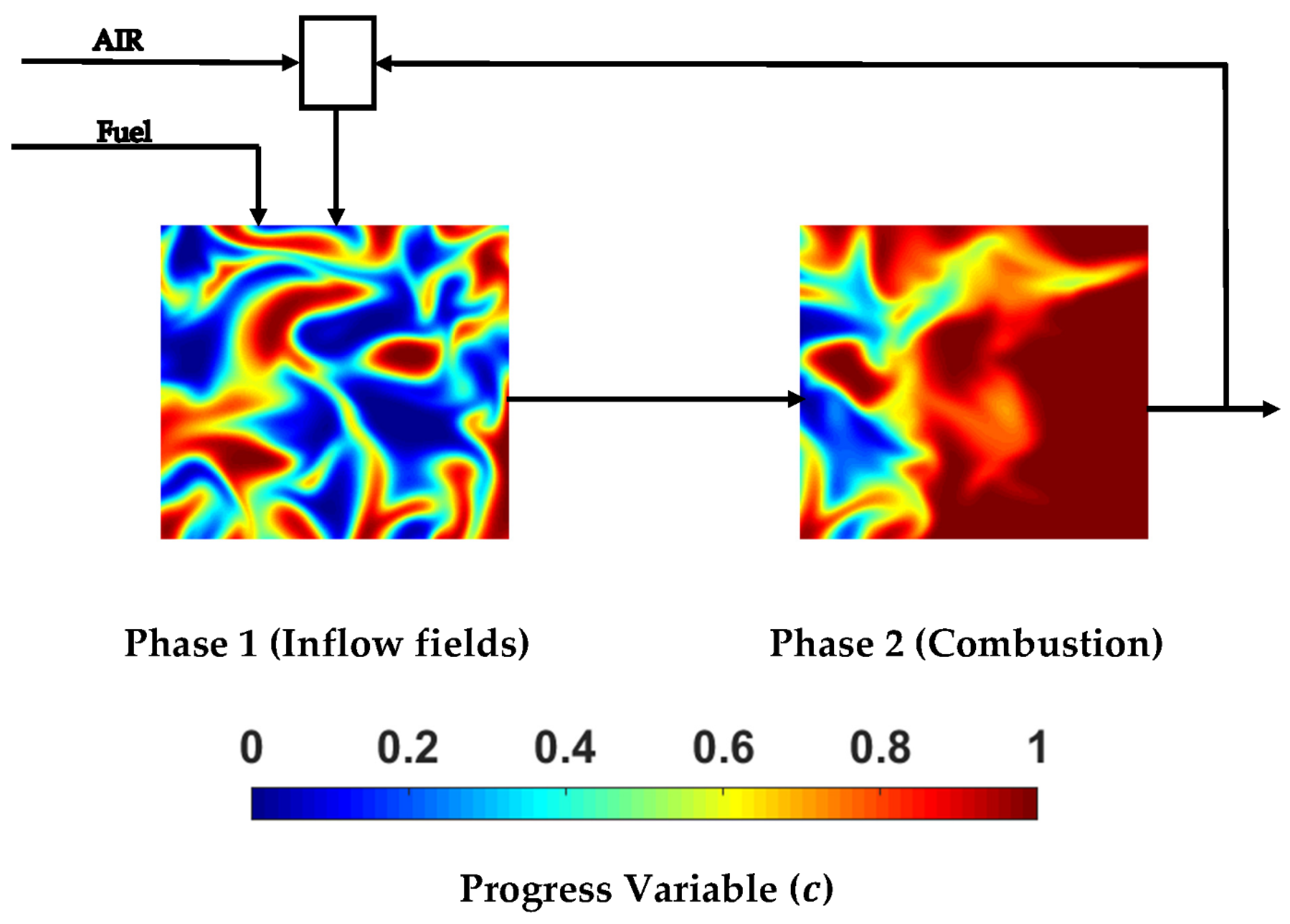
• The thermochemical conditions shown in Table 1 are used to simulate a 1D laminar premixed flame for $\varphi =0.8$. An initial bimodal distribution of $c_Y=1-Y_F/Y_{FR}$with prescribed integral length scale $l_{c }=1.50 \mathrm{mm}$ is then developed using the methodology by Eswaran and Pope [56]. The 1D laminar profiles of a species mass fraction for $\varphi =0.8$ are specified as a function of the progress variable $c_Y$. These functions, alongside the bimodal distribution of $c_Y$, are used to initialise the density and species mass fractions corresponding to an atmospheric pressure and an unburned gas temperature of 1500 K (i.e., $T_0=1500 \mathrm{K}$).
• The generated bimodal scalar fields in the previous step are then allowed to evolve with turbulence for about 1 turnover time $\left(l/u^{\prime }\right)$ in a periodic domain mimicking the EGR in MILD combustion. At the end of this step the mean and variance of the preprocessed $c$ field are $⟨c⟩\approx 0.50$ and $⟨{c^{\prime }}^2⟩\approx 0.09$ respectively where $⟨Q⟩$ is the mean value evaluated over the whole domain. The temperature in the preprocessed mixture has a variation of about $\pm 0.3\%$ of its mean value.
• The prepared mixture at the end of previous stage will then be fed into the domain through the inlet with a mean velocity $U_{in}=20 \mathrm{m}/\sec$ by scanning a plane through it, as used previously by Minamoto, Swaminathan and co-workers [19,20,21,22,23].

The species mass fractions, temperature and density for turbulent premixed flame simulations are initialised by the steady unstretched 1 D laminar premixed flame with $\varphi =0.8$. A pseudo-spectral method [54] is used to initialise turbulent velocity fluctuations by a homogeneous isotropic field with prescribed values of $u^{\prime }$ and $l$, according to Batchelor–Townsend spectrum [55].

The MILD combustion simulations were continued for 2.5 throughpass times (i.e., $t_{sim}=2.5L_x/U_{mean}$), amounting to $11, 16$ and$22$ initial eddy turn-over times (i.e., $11.0l/u^{\prime }, 16.0l/u^{\prime }$ and $22.0l/u^{\prime }$) for initial $u^{\prime }/S_L=4.0, 6.0$ and 8.0, respectively. The turbulent premixed flame simulations under decaying turbulence needed to be conducted for $t_{sim}=max\left(l/u^{\prime },{\delta }_{th}/S_L\right)$. In the present analysis, the premixed flame simulations were continued for one chemical timescale (i.e., $t_{sim}={\delta }_{th}/S_L$), amounting to $1.3, 2.0$ and $2.7$ initial eddy turn-over times (i.e., $1.3l/u^{\prime }, 2.0l/u^{\prime }$ and $2.7l/u^{\prime }$) for initial $u^{\prime }/S_L=4.0, 6.0$ and 8.0, respectively. By the time statistics were extracted, the flame surface area and volume-integrated reaction rate of the reaction progress variable had reached a quasi-steady state. These simulation times remain comparable to several previous studies [19,20,21,22,23,24,25,26,30,37,38,39], which contributed to the fundamental understanding and modelling of turbulent combustion in the past.

4. Results and Discussion

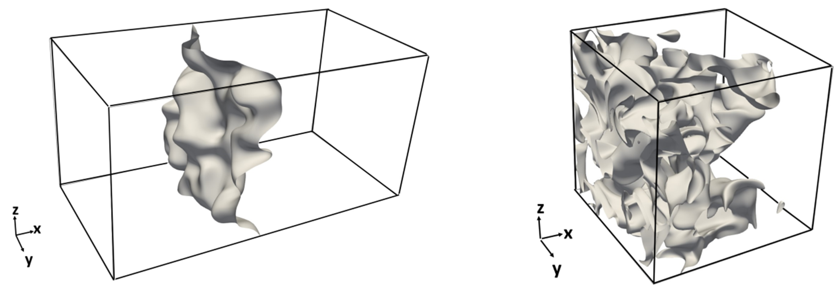
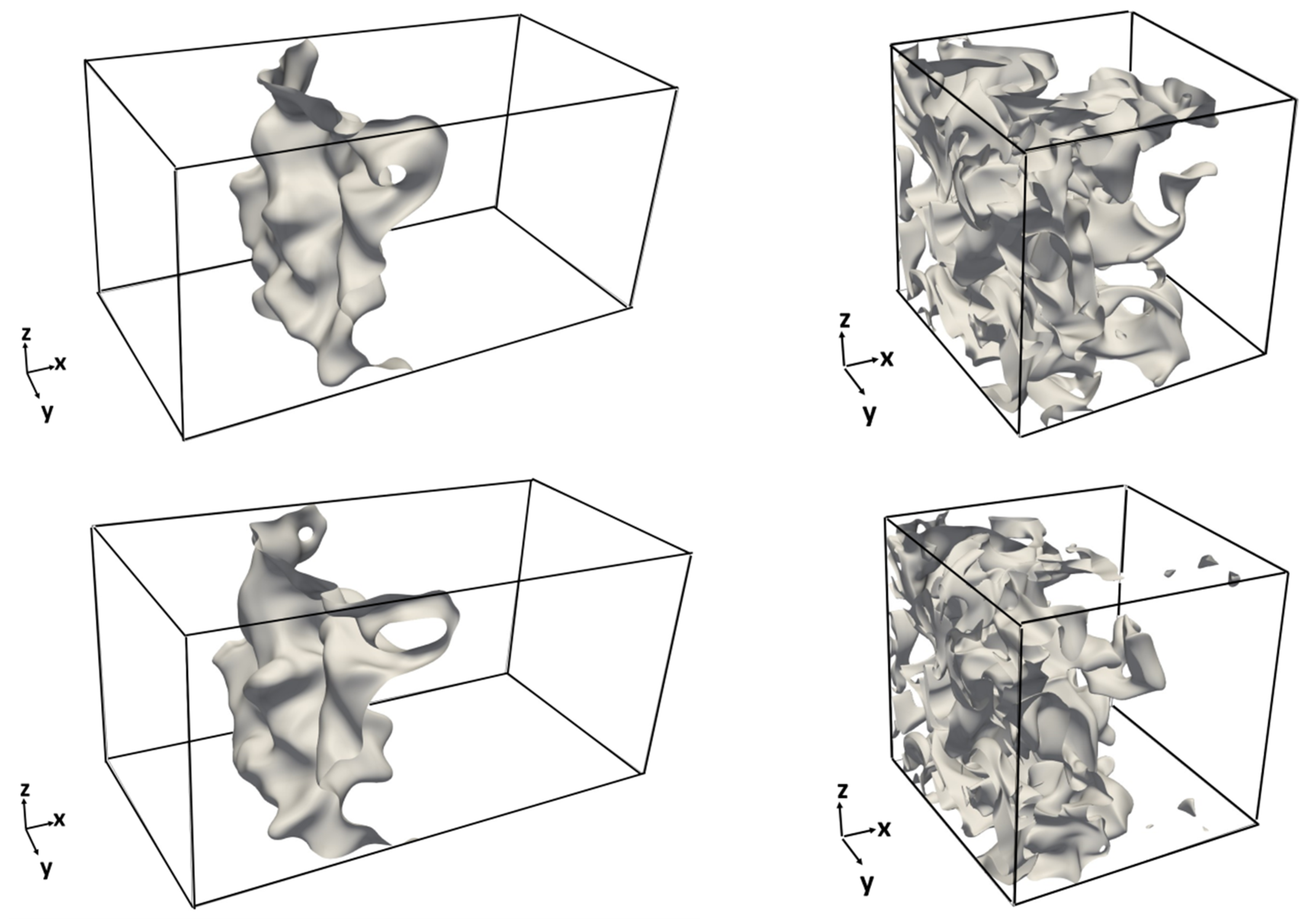
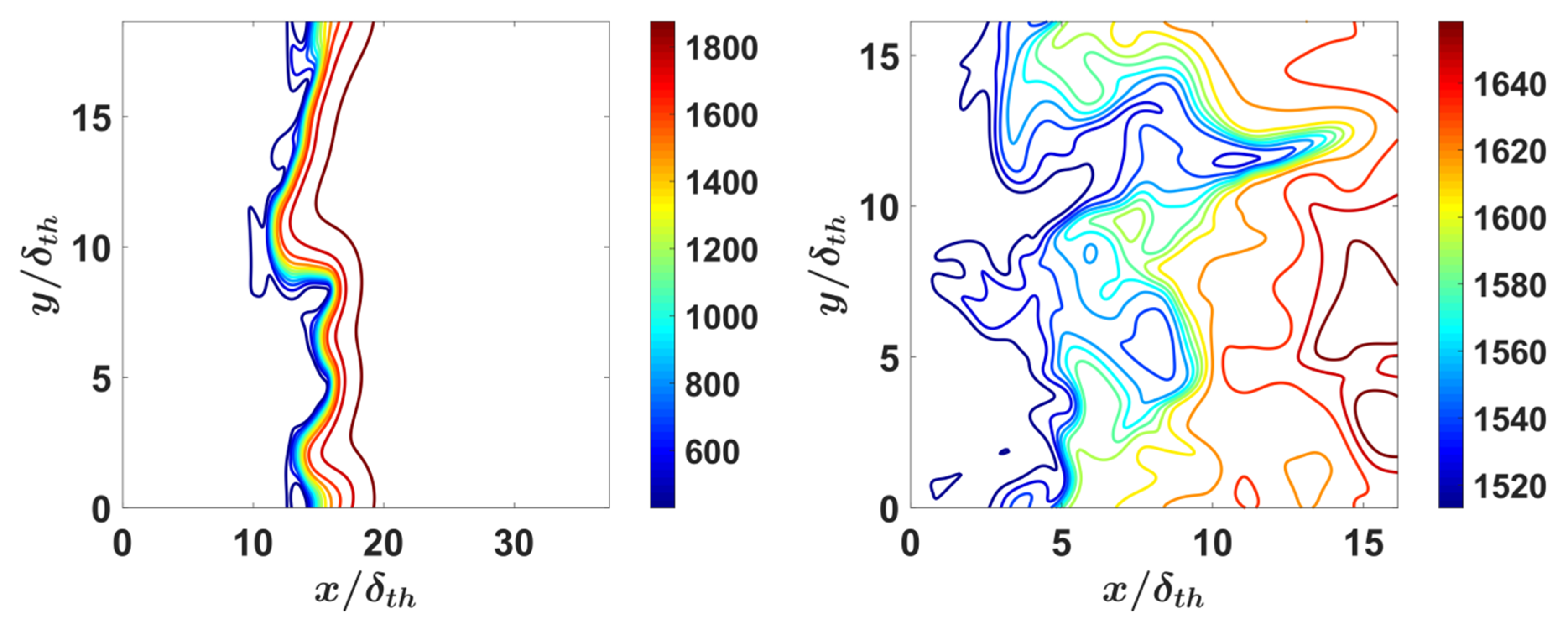
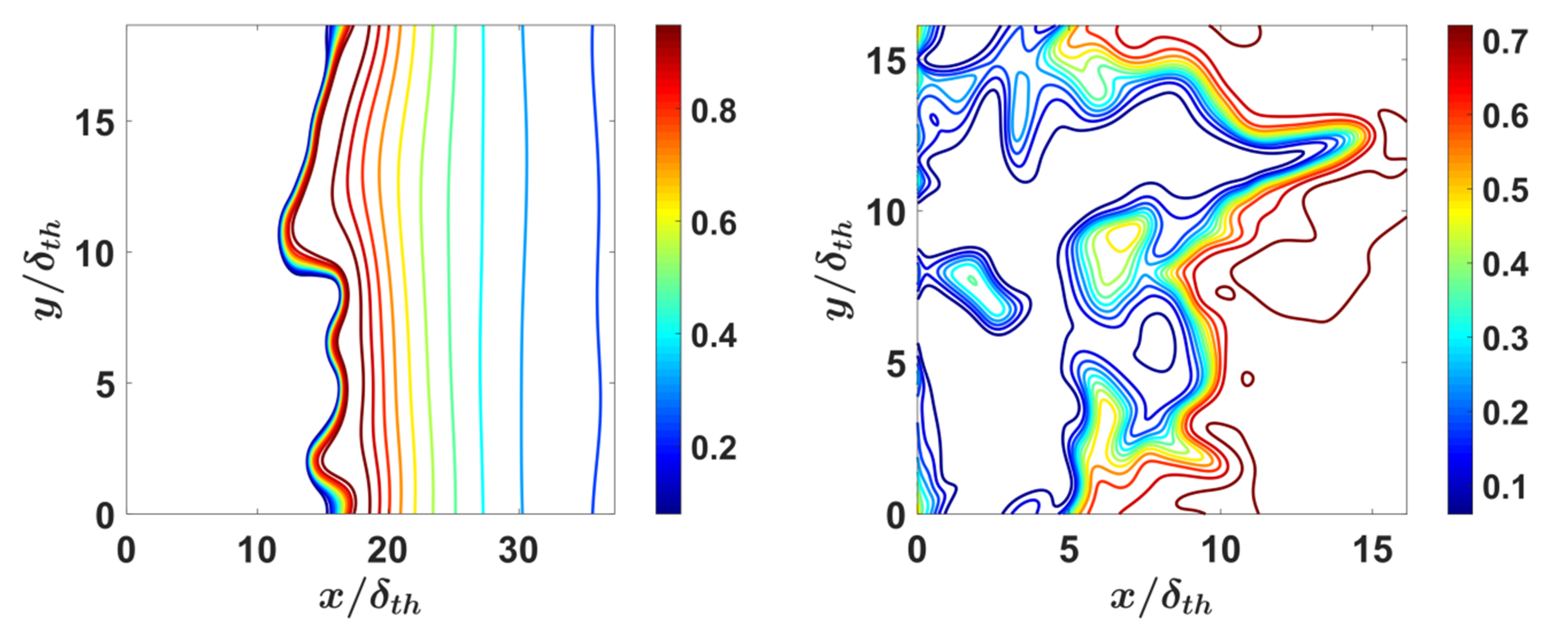
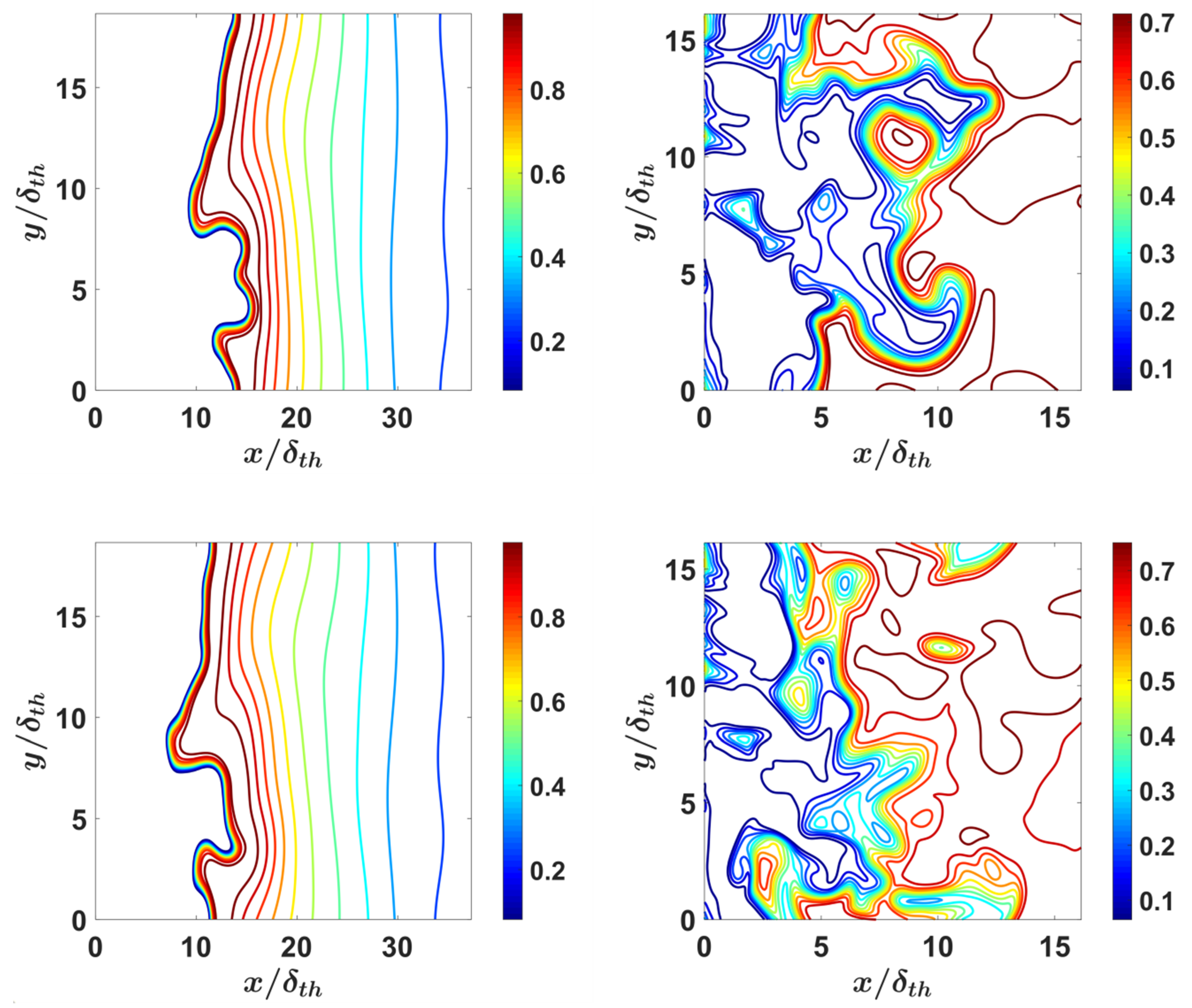
4.1. Flame Morphology

The instantaneous views of the $c=0.8$ isosurface, for both statistically planar turbulent premixed flames and homogeneous MILD combustion cases and for different turbulence intensities are shown in Figure 2. For methane–air combustion, the maximum heat release takes place close to $c=0.8$ for the unstretched laminar premixed flame, and thus the $c=0.8$ isosurface can be taken as a marker of the flame surface. It can be seen, from Figure 2, that the flame wrinkling increases with increasing $u^{\prime }/S_L$ for statistically planar turbulent premixed flames and, in these cases, the flame surface cleanly separates the reactants from the products, but the increased flame wrinkling, with an increase in $u^{\prime }/S_L$, may give rise to self-interactions between flame surface wrinkles that can lead to localised pockets. Figure 2 reveals that there are significant differences in flame morphologies between the homogeneous MILD combustion and premixed flame cases. There is a significant amount of self-interaction of the $c=0.8$ isosurface for all values of turbulence intensity in the MILD combustion cases and the extent of self-interaction increases with increasing turbulence intensity. The contours of temperature, $T$, in the central midplane for both the MILD and premixed cases considered here are shown in Figure 3, which reveals that the conventional premixed flame cases show a steep temperature gradient (from a temperature of 300 K in the reactants to 1960 K in the products) within the flame and the temperature contours become increasingly wrinkled with an increase in $u^{\prime }/S_L$. By contrast, the MILD combustion cases show a small change in temperature ($∆T\le 150 \mathrm{K}$) and thus the temperature rise is much more gradual in these cases than in the conventional premixed flames. The equivalent OH-PLIF signal constructed from DNS data can be evaluated in the following form for $1000 \mathrm{K}\le T\le 1800 \mathrm{K}$ [57,58,59,60,61]:

$$S_{\mathit{OH}}\propto X_{\mathit{OH}}{T}^{-\beta } where -2.6\le \beta \le 1.0$$

(11)

Here the value of $\beta$ is taken to be 0.0 (i.e., $\beta =0.0$) following previous studies [22]. The contours of $S_{OH}/{\left[S_{OH}\right]}_{max, L}$ at the central midplane for the cases considered here are shown in Figure 4, where ${\left[S_{OH}\right]}_{max, L}$ is the maximum value of the OH-PLIF signal in the corresponding unstretched laminar premixed flame. It can be seen from Figure 4 that the OH-PLIF signal reveals a much thicker reaction zone in MILD combustion cases than in the corresponding conventional premixed flames, but there is still a clearly defined interface separating reactants and products for turbulent MILD combustion. The observations made from temperature and the equivalent OH-PLIF signal from the DNS data are consistent with previous experimental [6,7,8,9,10,11,12,13,14,15] and numerical [19,20,21,22,23] findings.

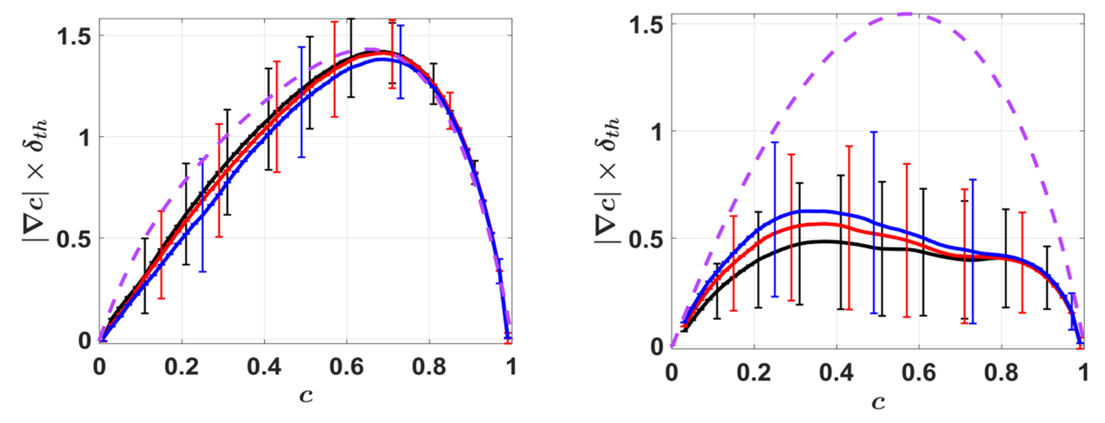
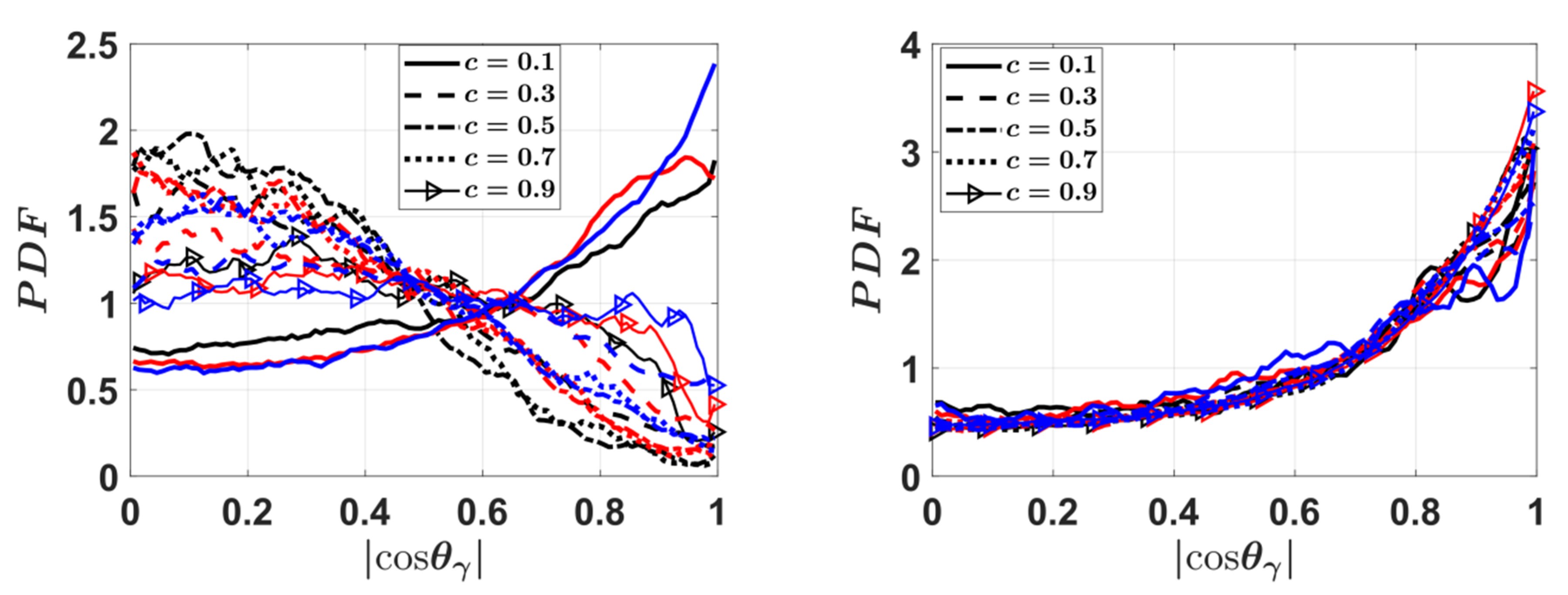
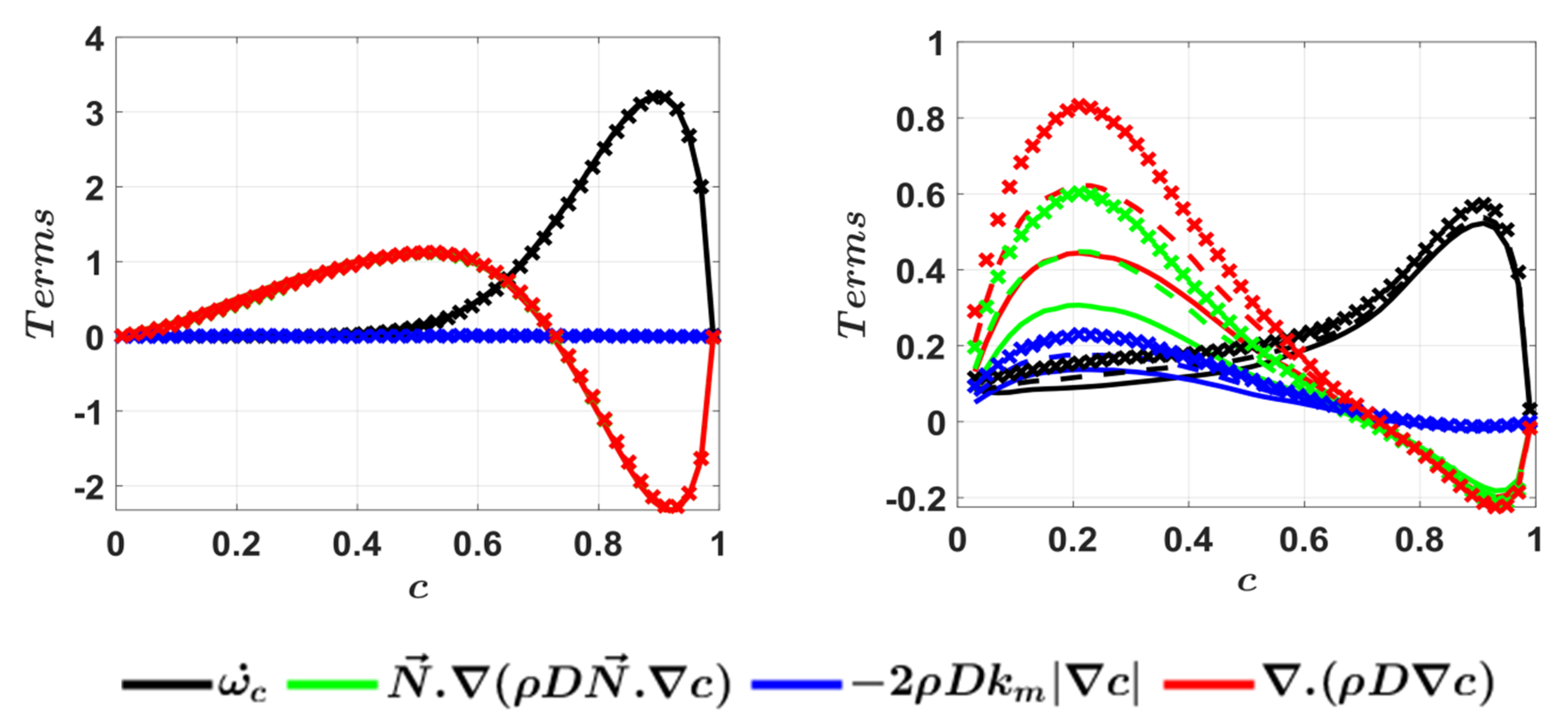
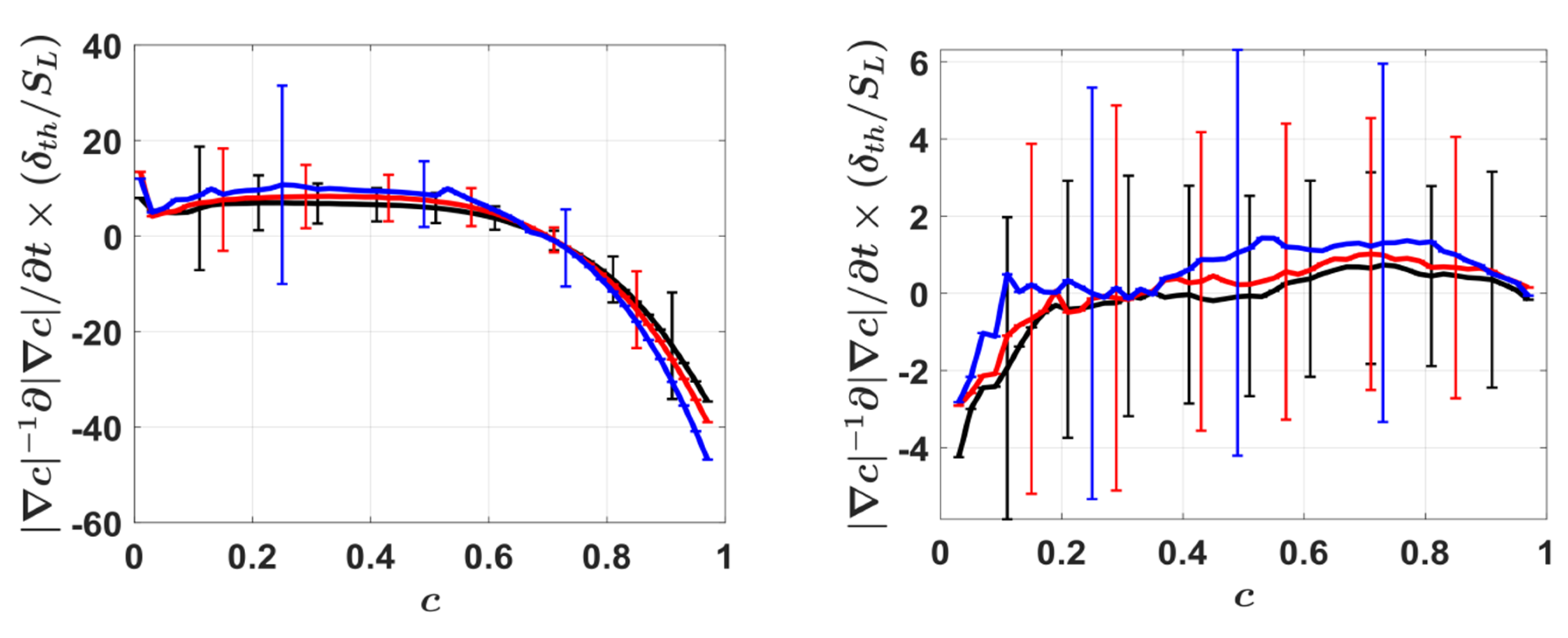
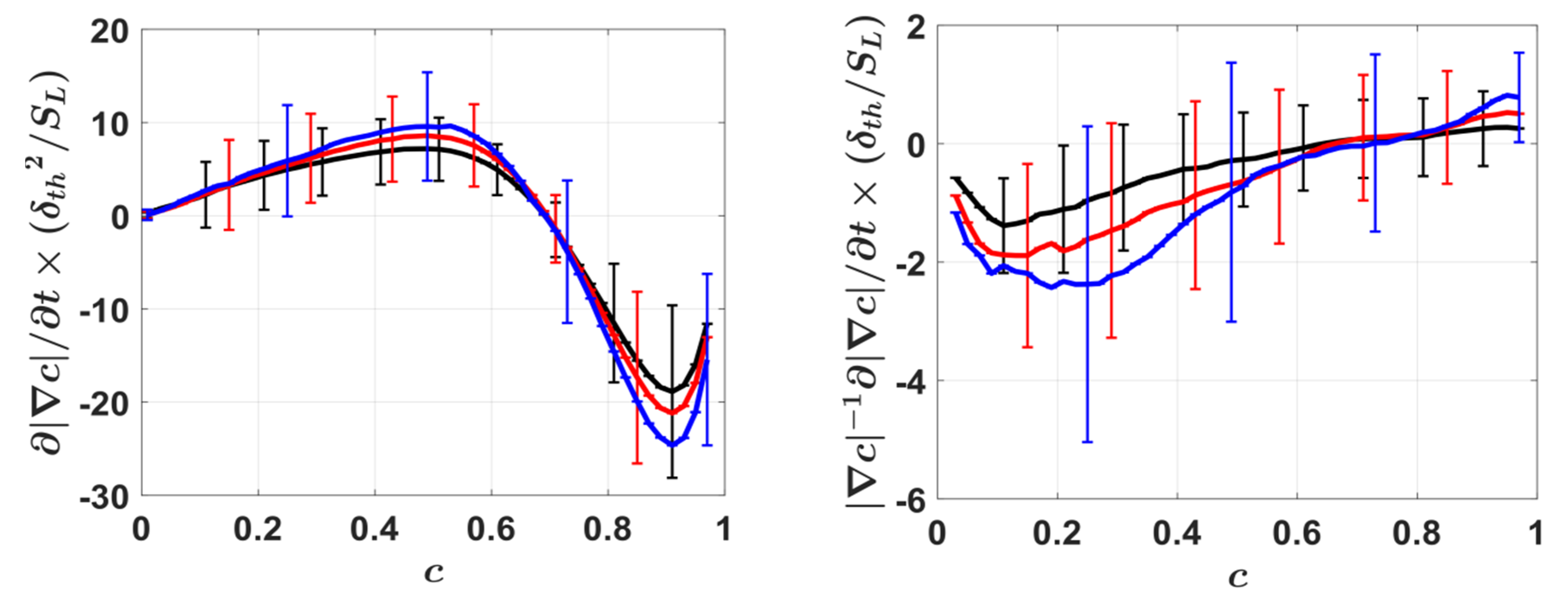
4.2. Mean Behaviour of the SDF

The mean values of the normalised SDF ($\left|\nabla c\right|\times {\delta }_{th}$) conditioned upon $c$ for both MILD and conventional premixed combustion cases, are shown in Figure 5, where the standard deviations of $\left|\nabla c\right|\times {\delta }_{th}$ conditioned upon $c$ are also shown. In contrast to premixed combustion, which shows that the peak mean value of the SDF is skewed towards the burned gas side, the MILD combustion cases show a $\left|\nabla c\right|\times {\delta }_{th}$ profile skewed towards the unburned gas side of the flame front. This is a consequence of the differences in reaction and diffusion contributions to the SDF evolution between MILD combustion cases and conventional premixed flames considered here. This is contingent on the maximum heat-release zone within the flame and highlights the difference between conventional premixed cases, where the maximum heat release occurs towards the burned gas side, in the range $c=0.7–0.8$, while in MILD combustion, the reaction contribution remains active for a broad range of reaction progress, variable across the flame front (see later in Figure 9). Moreover, the differences in molecular diffusion contribution (especially the flame tangential diffusion rate) between the premixed flames and MILD combustion cases also contribute to this (see Figure 9 later in this paper).

The inverse of the peak value of the mean value of $\left|\nabla c\right|$ conditioned upon $c$ provides the measure of the flame thickness (i.e., $\delta ~1/\max {⟨\left|\nabla c\right|⟩}_c$ where ${⟨\dots ⟩}_c$ is the mean value conditioned upon $c$) [32]. A comparison between the profiles of the MILD combustion and premixed flame cases reveals that the mean values of $\left|\nabla c\right|\times {\delta }_{\mathrm{th}}$ in MILD combustion cases remain smaller than those in the premixed flame cases, which is indicative of the thickened reaction zone separating reactants and products in contrast to a thin reaction zone in the premixed flame cases. This is also consistent with the observations made from Figure 2, Figure 3 and Figure 4. It can also be seen from Figure 5 that the maximum value of ${⟨\left|\nabla c\right|⟩}_c$ in the MILD combustion cases increases slightly with increasing $u^{\prime }/S_L$ but the differences between the mean values at different turbulence intensities remain much smaller than the standard deviation suggesting that differences in ${⟨\left|\nabla c\right|⟩}_c$ are not significant enough to imply any change in the thickness of the reaction zone under turbulent conditions. However, it can be seen from Figure 5 that the peak mean value of ${⟨\left|\nabla c\right|⟩}_c$ in the MILD combustion cases remains significantly smaller than the corresponding value in the 1D premixed flame case, indicating that the flame thickens considerably under turbulent conditions for the MILD combustion cases. The interactions of the flame surfaces in the MILD combustion cases, as shown in Figure 2, Figure 3 and Figure 4, contribute to this thickening of the flame under turbulent conditions. By contrast, the peak mean values of ${⟨\left|\nabla c\right|⟩}_c$ for both laminar and turbulent conditions are almost identical to each other for the conventional premixed flame cases. Figure 5 also shows that the peak value of ${⟨\left|\nabla c\right|⟩}_c$ for the turbulent premixed flame cases do not change significantly with a change in $u^{\prime }/S_L$, but a small decrease in the peak value of ${⟨\left|\nabla c\right|⟩}_c$ is discerned with an increase in $u^{\prime }/S_L$. However, the standard deviations of $\left|\nabla c\right|$ in the premixed flame cases also remain greater than the differences in mean values and, therefore, the differences in the mean values of $\left|\nabla c\right|$ do not signify a change in the mean flame thickness in response to the variation in turbulence intensity within the parameter range considered here. Moreover, comparable peak mean values of ${⟨\left|\nabla c\right|⟩}_c$, for both the laminar and turbulent conditions in conventional premixed flame cases, suggest that the flame thickness does not change significantly under turbulent conditions. However, an increase in $u^{\prime }/S_L$ increases the standard deviation of $\left|\nabla c\right|$, since the range of fluctuation increases with increasing turbulence intensity. It is worthwhile to analyse the strain rates, which affect the evolution of the SDF (see Equation (9)), to explain the observed behaviours of $\left|\nabla c\right|$ in both premixed flame and MILD combustion cases.

4.3. Mean Behaviour of Fluid-Dynamic Strain Rates

The profiles of the mean values of $\{a_N, a_T$and $\nabla ·\overrightarrow{u}\}\times {\delta }_{th}/S_L$ conditioned upon $c$ are presented in Figure 6. The dilatation rate $\nabla ·\overrightarrow{u}$ assumes positive values because of the thermal expansion due to heat release for both the premixed and MILD flame cases but the mean values of $\nabla ·\overrightarrow{u}\times {\delta }_{th}/S_L$, in the MILD combustion cases, remain negligibly small in comparison with the premixed flame cases. This suggests that the thermal expansion effects are relatively weak in the MILD combustion cases compared with conventional premixed flames. In the premixed flames, the peak mean value of $\nabla ·\overrightarrow{u}\times {\delta }_{th}/S_L$ is obtained in the middle of the flame with a skewness towards the burned gas side (i.e., $c\approx 0.65$), whereas the mean value of $\nabla ·\overrightarrow{u}\times {\delta }_{th}/S_L$ remains vanishingly small for all $c$ values in the MILD combustion cases.

It can be seen from Figure 6 that the mean value of $a_N$ remains negative towards the unburned gas side of the flame, while positive values are obtained for larger values of $c$ in the premixed flame cases. The normal strain rate $a_N$ can be expressed as [41,42,43,44,62]:

$${ a}_N=(e_{\alpha }{\cos }^2{\theta }_{\alpha }+e_{\beta }{\cos }^2{\theta }_{\beta }+e_{\gamma }{\cos }^2{\theta }_{\gamma })$$

(12)

where $e_{\alpha },e_{\beta }$ and $e_{\gamma }$ are the most extensive, intermediate and the most compressive principal strain rates, respectively and ${\theta }_{\alpha }, {\theta }_{\beta }$ and ${\theta }_{\gamma }$ are the angles between $\nabla c$ with eigendirections corresponding to $e_{\alpha },e_{\beta }$ and $e_{\gamma }$, respectively. The PDFs of $\left|\cos {\theta }_{\alpha }\right|, \left|\cos {\theta }_{\beta }\right|$ and $\left|\cos {\theta }_{\gamma }\right|$ for different $c-$ isolevels across the flame for both MILD combustion and premixed flame cases considered here are shown in Figure 7. A high probability of $\left|\cos {\theta }_i\right|=1.0$ (for $i=\alpha ,\beta ,\gamma$) indicates a preferential collinear alignment between $\nabla c$ with the eigenvector associated with $e_i$ (for $i=\alpha ,\beta ,\gamma$). Figure 7 shows that the reaction progress variable gradient, $\nabla c,$ preferentially aligns collinearly with the most compressive principal strain rate eigendirection throughout the flame in the MILD combustion cases, similarly to passive scalar mixing [63,64,65,66,67,68,69,70,71,72], and a preferential collinear alignment between $\nabla c$ and the eigenvector associated with $e_{\gamma }$, in the premixed flame cases, are observed towards the unburned and burned gas sides of the flame where the effects of heat release are weak. However, it can be seen from Figure 7 that $\nabla c$ preferentially collinearly aligns with the most extensive principal strain rate eigendirection in the region of the flame, where the effects of thermal expansion are strong (i.e., where dilatation rate assumes large values) in the premixed flame cases. In the case of passive scalar mixing, $\nabla c$ preferentially collinearly aligns with the most compressive principal strain rate eigendirection [63,64,65,66,67,68,69,70,71,72], whereas, in premixed flames, $\nabla c$ may align preferentially with the most extensive principal strain rate eigendirection if the strain rate induced by flame normal acceleration overcomes turbulent straining [62,72]. The strain rate induced by flame normal acceleration $a_{chem}$ can be taken to scale with $\tau S_L/{\delta }_{th}$ (where $\tau ={\rho }_u/{\rho }_b-1$ is the heat release parameter with ${\rho }_u$ and ${\rho }_b$ are the unburned gas density and the burned gas density, respectively) [62], whereas large-scale turbulent straining is given by $a_{turb}~u^{\prime }/l$. This suggests that $\nabla c$ aligns preferentially with the most extensive principal strain rate eigendirection for $\tau S_L/{\delta }_{th}\gg u^{\prime }/l$, which is characterised by $\tau Da\gg 1$. By contrast, $\nabla c$ aligns preferentially with the most compressive principal strain rate eigendirection for $\tau S_L/{\delta }_{th}\ll u^{\prime }/l$, which is characterised by $\tau Da\ll 1$. For MILD combustion cases, $\tau Da$ remains small due to small values of $\tau$ and thus a preferential alignment of $\nabla c$ with the most compressive principal strain rate eigendirection is observed in these cases, leading to predominantly negative values of $a_N$, according to Equation (12). This tendency strengthens with an increase in $u^{\prime }/S_L$, as a result of the reduction in $Da$, and therefore, the mean value of $a_N$ assumes negative values of higher magnitudes for higher values of $u^{\prime }/S_L$ (see Figure 6).

For the premixed flame cases considered here, $\tau Da$ remains greater than 1.0 (i.e., $\tau Da>1$) and thus, a preferential alignment of $\nabla c$ with the most extensive principal strain rate eigendirection is observed within a major part of the flame in these cases, leading to predominantly positive values of $a_N$, according to Equation (12). This is valid in the regions of heat release, but an increase in $u^{\prime }/S_L$ leads to a drop in $Da$, which reduces the extent of the preferential alignment of $\nabla c$ with the most extensive principal strain rate eigendirection leading to a marginal decrease in the positive mean values of $a_N$ with an increase in $u^{\prime }/S_L$ in the premixed flame cases.

As the dilatation rate $\nabla ·\overrightarrow{u}$ is vanishingly small in the MILD combustion cases, the predominantly negative mean values of $a_N$ lead to positive mean values of tangential strain rate $a_T=\nabla ·\overrightarrow{u}-a_N$ in these cases. In the premixed flames considered here, the mean value of $\nabla ·\overrightarrow{u}$ remains greater than that of $a_N$, which leads to positive mean values of $a_T$ throughout the flame. As the mean value of $\nabla ·\overrightarrow{u}$ is primarily determined by thermochemistry, the decrease in mean values of $a_N$ with increasing $u^{\prime }/S_L$ leads to an increase in the mean value of tangential strain rate $a_T=\nabla ·\overrightarrow{u}-a_N$. The positive mean value of $a_T$ is indicative of flame area generation under fluid-dynamic straining in all the cases considered here.

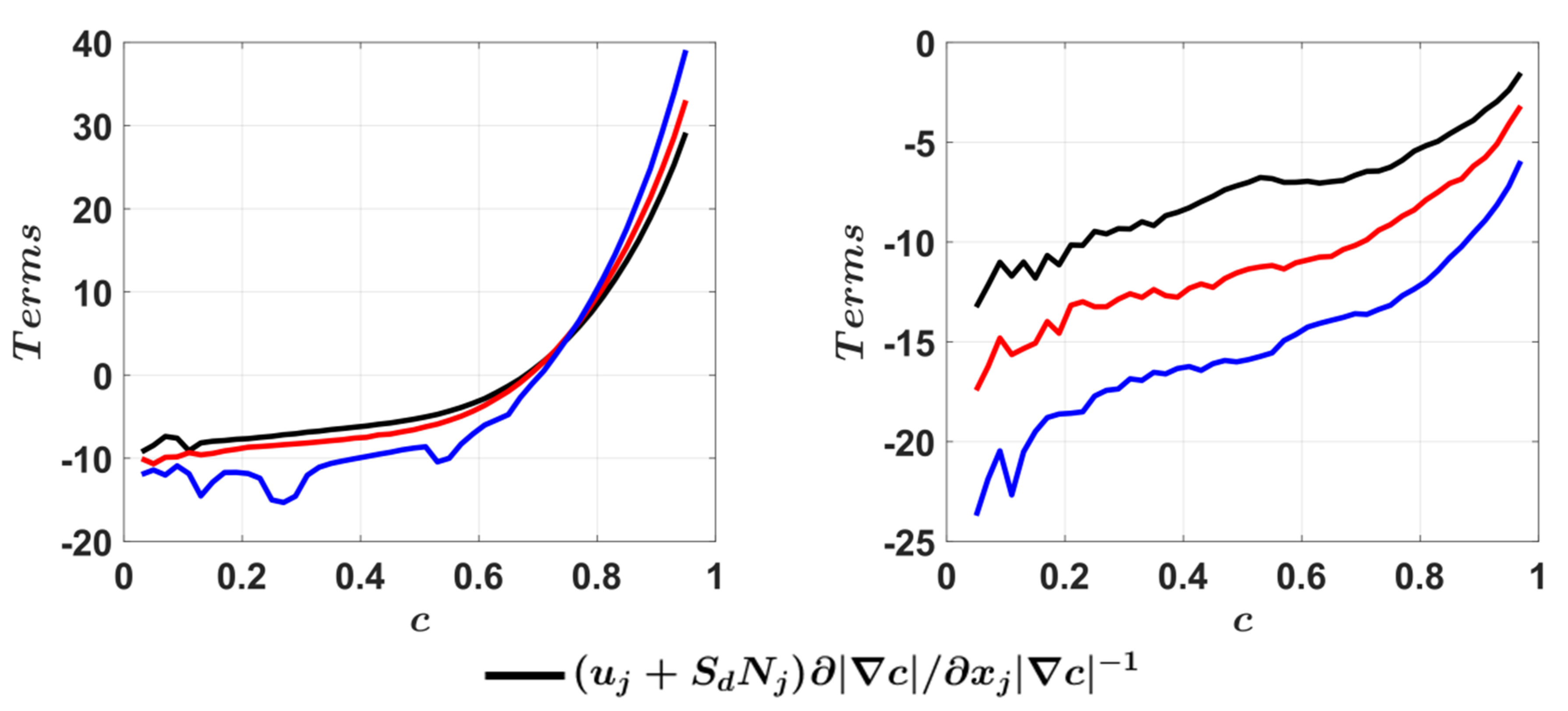
4.4. Mean Behaviour of Flame Displacement Speed

It is evident from Equations (9) and (10) that the strain rates due to flame propagation are closely related to the flame displacement speed, $S_d$. The mean values of $S_d/S_L$ and its components (i.e., $S_r/S_L, S_n/S_L$ and $S_t/S_L$), conditioned upon $c$, are shown in Figure 8 for the cases considered here. In order to understand the statistics of displacement speed and its components, the mean values of $\{{\dot{\omega }}_c, \overrightarrow{N}·\nabla (\rho D\overrightarrow{N}·\nabla c), \nabla ·(\rho D \nabla c)$ and $-2\rho D{\kappa }_m\left|\nabla c\right|\}\times {\delta }_{th}/{\rho }_0{S}_L$ conditioned upon $c$ are presented in Figure 9.

It can be seen from Figure 9 that the mean value of ${\dot{\omega }}_c\times {\delta }_{th}/{\rho }_u{S}_L$ peaks towards the burned gas side of the flame for both MILD combustion and conventional premixed flames. However, it can be seen from Figure 8 and Figure 9 that the mean value of ${\dot{\omega }}_c\times {\delta }_{th}/{\rho }_u{S}_L$, and, accordingly, of $S_r/S_L$, assume non-negligible values in MILD combustion for a broader range of $c$ than in the conventional premixed flame cases. The unburned gas temperature in MILD combustion cases is above the autoignition temperature, which gives rise to non-negligible reaction rates ${\dot{\omega }}_c$ for the unburned gas side of the flame-front, whereas the reaction rate ${\dot{\omega }}_c$ and thereby also the reaction component of displacement speed $S_r$ for conventional premixed flames assume non-negligible values only for $c>0.5$.

The mean value of the flame normal diffusion rate $\overrightarrow{N}·\nabla (\rho D\overrightarrow{N}·\nabla c)$ is positive towards the unburned gas side but becomes negative on the burned gas side of the flame for both the MILD combustion and conventional premixed flame cases, and therefore the mean normal diffusion component of displacement speed, $S_n$, also assumes positive (negative) mean values for the unburned (burned) gas side of the flame. The magnitude of the mean contribution of $-2\rho D{\kappa }_m\left|\nabla c\right|$ remains small in comparison to the leading order mean contributions of ${\dot{\omega }}_c$ and $\overrightarrow{N}·\nabla (\rho D\overrightarrow{N}·\nabla c)$ for all cases considered in this analysis (see Figure 9). This is due to the statistically planar nature of these cases. Accordingly, the mean value of $S_t$ remains negligible in comparison to the mean values of $S_r$ and $S_n$ for both premixed and MILD combustion cases. Thus, $S_r$ and $S_n$ are the major contributors to the mean values of $S_d$ for all cases considered here. However, there are differences in the mean behaviours of $S_r$ and $S_n$ between premixed flame and MILD combustion cases. Figure 9 indicates the mean values of ${\dot{\omega }}_c$ and $\overrightarrow{N}·\nabla (\rho D\overrightarrow{N}·\nabla c)$ (and also $\nabla \left(\rho D\nabla c\right)$) remain of the same order of magnitude but with different signs in the reaction zone, and, accordingly, the mean values of $S_r$ and $S_n$ are of the same order in the reaction zone both in the premixed flame and MILD combustion cases. It is important to note that ${\delta }_{th}/{\rho }_u{S}_L$, in the MILD combustion cases, is a factor of 2.0 smaller than the premixed flame cases considered here. Therefore, the magnitudes of ${\dot{\omega }}_c$ and $\overrightarrow{N}·\nabla (\rho D\overrightarrow{N}·\nabla c)$ for the conventional premixed flame and MILD combustion cases remain comparable in spite of the differences in their normalised values (i.e., ${\dot{\omega }}_c\times {\delta }_{th}/{\rho }_u{S}_L$ and $\overrightarrow{N}·\nabla (\rho D\overrightarrow{N}·\nabla c)\times {\delta }_{th}/{\rho }_u{S}_L$) between MILD combustion and conventional premixed flame cases in Figure 9. However, the relative magnitudes of mean $S_r$ and $S_n$ are such that the mean $S_d$ increases with increasing $c$ in turbulent premixed flames, whereas the positive contribution of ${\dot{\omega }}_c$ is partially nullified by the negative contribution of $\overrightarrow{N}·\nabla (\rho D\overrightarrow{N}·\nabla c)$ in the MILD combustion cases in such a manner that the mean displacement speed $S_d$ decreases from the unburned gas side to the middle of the flame and subsequently increases mildly with $c$ for $c>0.6$ (see Figure 8). Moreover, it can be seen from Figure 8 that the mean $S_d$ is not affected by turbulence intensity in the premixed flame cases. The statistical behaviour of $S_d$ and the differences in its behaviour between premixed flames and MILD combustion cases, in turn, affect the strain rates induced by flame propagation. Although the mean values of $S_d/S_L$ in the MILD combustion cases are comparable for the conventional premixed flame and MILD combustion cases, the higher value of $S_L$ in the MILD combustion cases implies higher magnitude of $S_d$ in these cases in comparison to that in the conventional premixed flame cases.

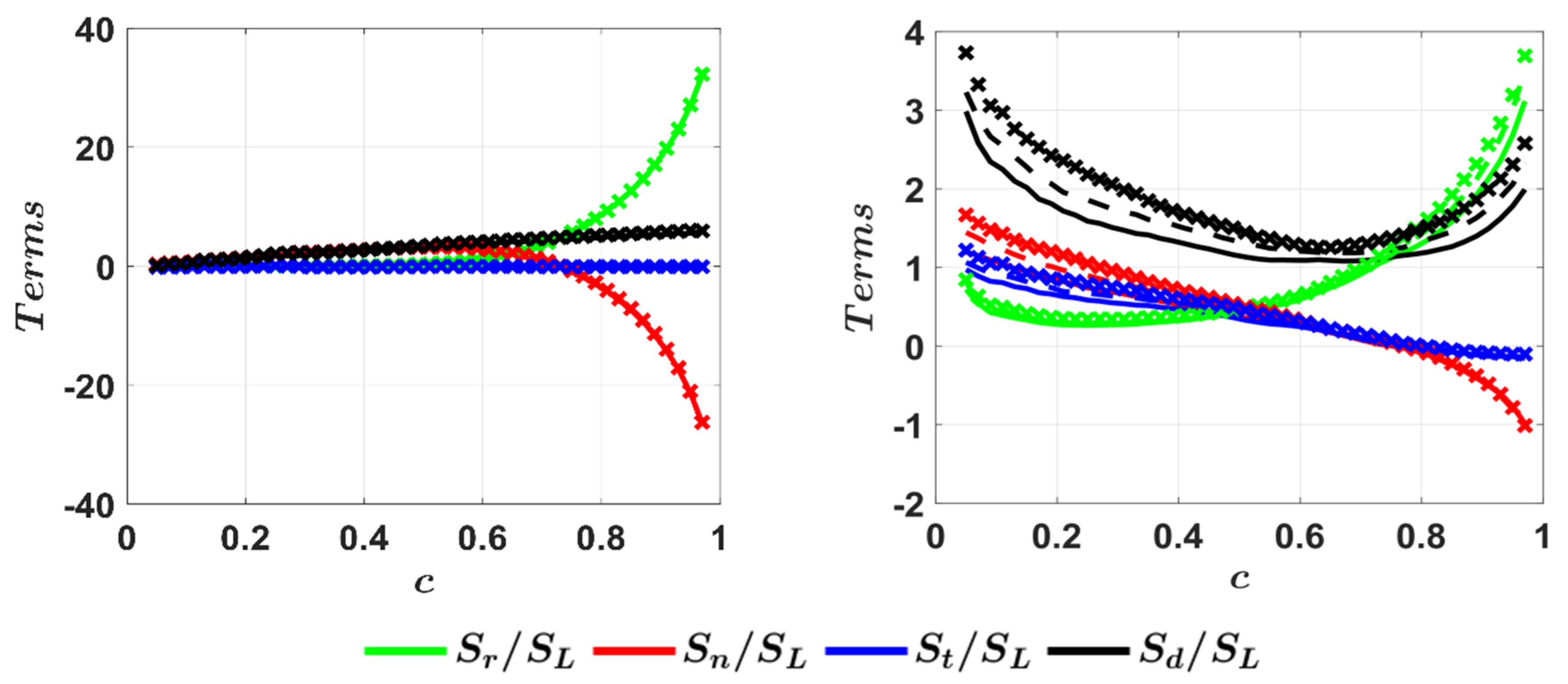
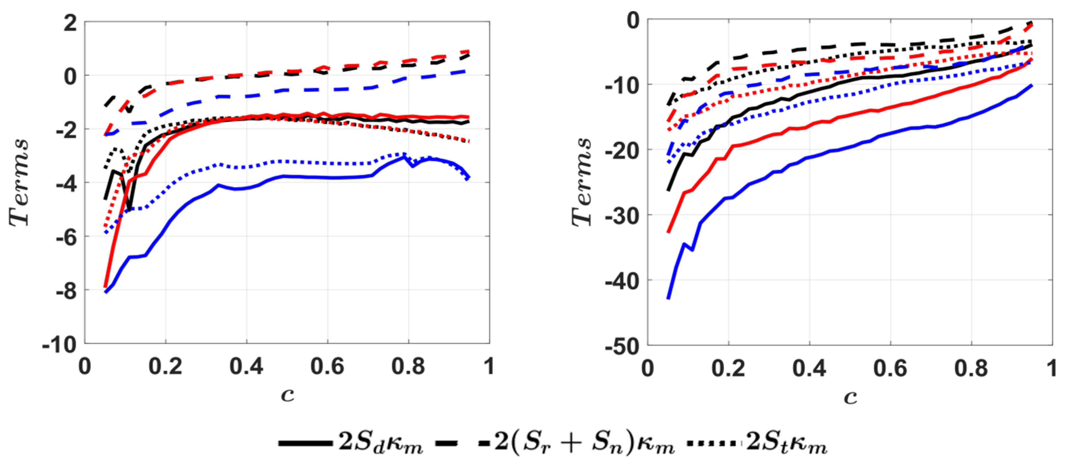
4.5. Mean Behaviour of Strain Rates Induced by Flame Propagation

The profiles of the normalised mean values of the additional flame normal strain rate due to flame propagation ($N_j\partial S_d/\partial x_j\times {\delta }_{th}/ S_L$) and its components (i.e., $N_j\partial (S_r+S_n)/\partial x_j\times {\delta }_{th}/ S_L$ and $N_j\partial S_t/\partial x_j\times {\delta }_{th}/ S_L$) conditioned upon $c$ are shown in Figure 10. It is worth noting that ${\delta }_{th}$ values for the conventional premixed flame and MILD combustion cases remain comparable [20,21] but $S_L$ values are significantly different, so the chemical timescale ${\delta }_{th}/ S_L$ in the MILD combustion cases remains almost 1/10 of the corresponding value in the premixed flame cases. This suggests that $N_j\partial S_d/\partial x_j$ and its components assume larger magnitudes in the MILD combustion cases than in the conventional premixed flames. The higher magnitude of displacement speed in the MILD combustion cases and comparable values of flame thickness contribute to larger magnitudes of mean values of $N_j\partial S_d/\partial x_j$ and its components in the MILD combustion cases than those in the premixed flame cases. It can further be seen from Figure 10 that the mean value of $N_j\partial S_d/\partial x_j$ remains positive towards the unburned gas side but assumes negative values for a major part of the flame front in the premixed flame cases because the mean value of $S_d$ increases with increasing $c$, which is consistent with previous studies [41,42,43]. The mean contribution of $N_j\partial S_d/\partial x_j$ assumes positive values throughout the flame in the MILD combustion cases because of the qualitatively different variation of $S_d$ in comparison to the corresponding premixed flame cases (see Figure 5). It can also be seen from Figure 10 that the mean value of $N_j\partial S_d/\partial x_j$ is principally driven by the mean contribution of $N_j\partial (S_r+S_n)/\partial x_j$ in the premixed flame cases. However, it is worth noting that the local curvature variations give rise to non-negligible positive mean value of $N_j\partial S_t/\partial x_j$ for the premixed flame cases. In MILD combustion cases, the contribution of $N_j\partial S_t/\partial x_j$ assumes positive values across the whole range of $c$ values and is of the same order of magnitude as $N_j\partial (S_r+S_n)/\partial x_j$. As the extent of flame curvature variation increases with increasing turbulence intensity, the magnitude of $N_j\partial S_t/\partial x_j=-2N_j\partial (D_c{\kappa }_m)/\partial x_j$ increases with increasing $u^{\prime }/S_L$. The diffusivity, $D_c$, increase from the unburned to the burned gas side of premixed flames acts to promote negative values of $N_j\partial (D_c{\kappa }_m)/\partial x_j$, which eventually leads to positive mean values of $N_j\partial S_t/\partial x_j=-2N_j\partial (D_c{\kappa }_m)/\partial x_j$. The effects of the increase in $D_c$ remain weak in the MILD combustion cases and a decrease in flame curvature towards the burned gas side, due to the weakening of turbulence, induces predominantly positive values of $N_j\partial (D_c{\kappa }_m)/\partial x_j$, which eventually leads to a decrease in the mean values of $N_j\partial S_t/\partial x_j=-2N_j\partial (D_c{\kappa }_m)/\partial x_j$ towards the burned gas side of these cases. The mean values of $N_j\partial (S_r+S_n)/\partial x_j$ for the turbulent premixed flame cases remain comparable for all the turbulence intensities considered in this analysis. However, the higher positive mean value of $N_j\partial S_t/\partial x_j$ in the premixed flame case with initial $u^{\prime }/S_L=8.0$ gives rise to a smaller negative mean value of $N_j\partial S_d/\partial x_j$ than in cases with initial $u^{\prime }/S_L=4.0$ and 6.0. As the mean value of $S_d$ is significantly affected by turbulence intensity in MILD combustion cases, the mean value of $N_j\partial S_d/\partial x_j$ also shows significant $u^{\prime }/S_L$ dependence and the mean value of positive contribution of $N_j\partial S_d/\partial x_j$ increases with increasing $u^{\prime }/S_L$. According to Equation (9), a negative (positive) $N_j\partial S_d/\partial x_j$ tends to promote flame thinning (flame thickening) and therefore the mean contribution of the additional normal strain rate $N_j\partial S_d/\partial x_j$ to the SDF evolution is different in the MILD combustion cases in comparison with the conventional premixed flame. The relative magnitudes of the mean values of $a_N$ and $N_j\partial S_d/\partial x_j$ determine the mean behaviour of the effective normal strain rate $a_N^{eff}$.

The profiles of the normalised mean values of the additional flame tangential strain rate due to flame propagation (i.e., alternatively curvature stretch rate given by $2S_d{\kappa }_m\times {\delta }_{th}/ S_L$) and its components conditioned upon $c$ are shown in Figure 11. It can be seen from Figure 11 that the mean value of $2S_d{\kappa }_m$ remains negative for both conventional premixed flames, and MILD combustion cases considered here. In all cases the negative definite value of $2S_t{\kappa }_m=-4D_c{\kappa }_m^2$ is the major contributor to the mean value of curvature stretch $2S_d{\kappa }_m$. This is consistent with the scaling arguments by Peters [53], suggesting that the stretch rate induced by the tangential diffusion component of displacement speed is the dominant component of $2S_d{\kappa }_m$ for $Ka\gg 1$ cases, as in the cases considered here. The mean value of $2(S_r+S_n){\kappa }_m$ increases from the unburned gas side to the burned gas side for both conventional premixed flames and MILD combustion cases considered here, but this contribution is dominated by the negative contribution of $2S_t{\kappa }_m=-4D_c{\kappa }_m^2$. The negative mean values of $2S_d{\kappa }_m$ indicate that the curvature stretch in the cases considered here act to reduce the flame area generation under turbulence for all cases considered here. However, there are qualitative differences in the variations of the mean values of $2S_d{\kappa }_m$ between the MILD combustion and conventional premixed flame cases. In the conventional premixed flame cases, the mean value of $2S_d{\kappa }_m$ does not alter significantly across a major part of the flame-front, whereas the magnitude of the negative mean value of $2S_d{\kappa }_m$ in the MILD combustion cases decreases from the unburned to the burned gas side. As the extent of flame wrinkling increases with increasing turbulence intensity, a larger range of curvature is obtained for higher values of turbulence intensity, which acts to increase the magnitude of $2S_t{\kappa }_m=-4D_c{\kappa }_m^2$ with an increase in $u^{\prime }/S_L$. As ${\delta }_{th}/ S_L$ in the MILD combustion cases remains almost 1/10 of the corresponding value in the premixed flame cases, the magnitudes of $2S_t{\kappa }_m$ and $2S_d{\kappa }_m$, in the MILD combustion cases, are greater than those in the conventional premixed flames. The higher magnitude of displacement speed and greater extent of flame wrinkling (i.e., larger spread of curvature values) in the MILD combustion cases contribute to larger magnitudes of $2S_t{\kappa }_m$ and $2S_d{\kappa }_m$ in these cases than in the premixed flame cases.

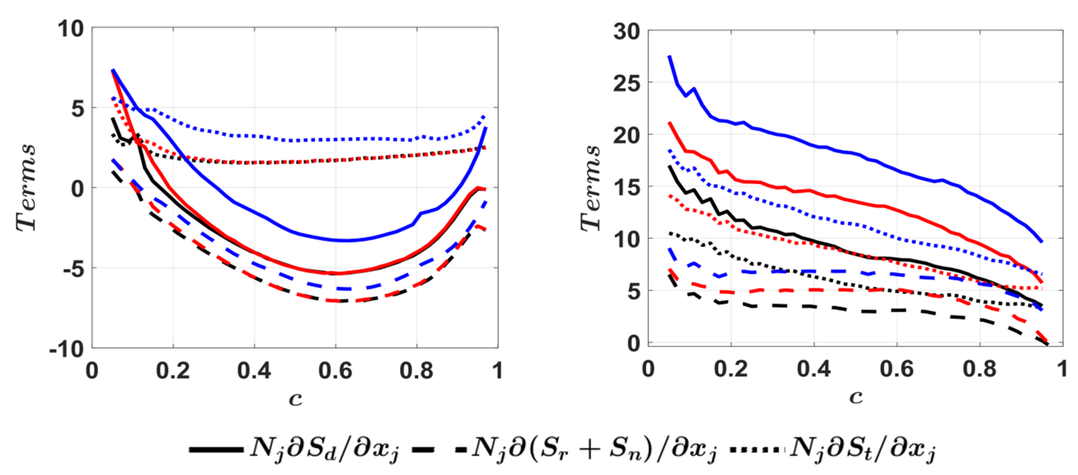
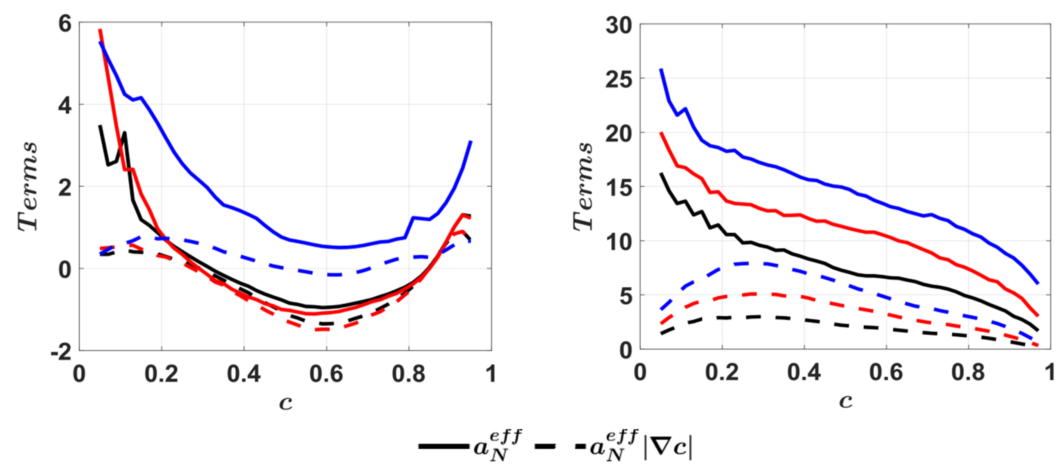
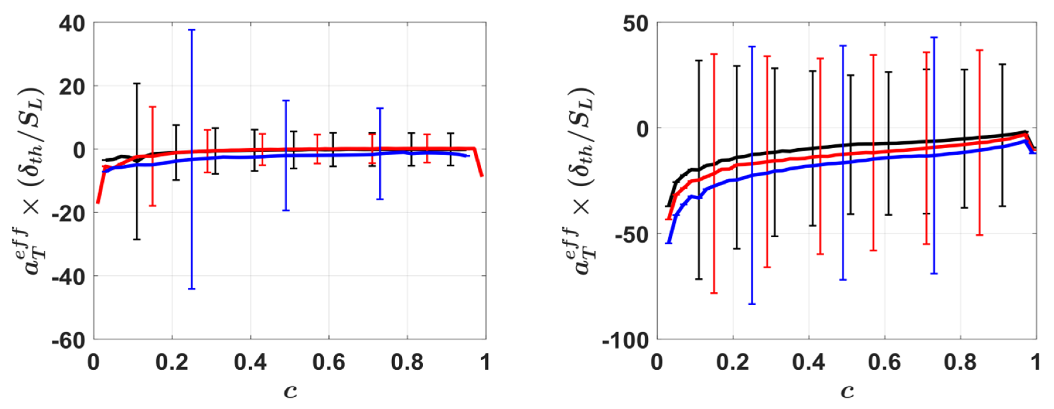
4.6. Mean Behaviour of Effective Strain Rates

The profiles of the normalised mean values of the effective normal rate $a_N^{eff}\times {\delta }_{th}/S_L$ conditioned upon $c$ are shown in Figure 12. According to Equation (9), a positive value of $a_N^{eff}$ at low values of $c$ indicates that there is a propensity for a decrease in $\left|\nabla c\right|$, while a negative effective normal strain rate at high values of $c$ gives rise to an increase in $\left|\nabla c\right|$. For the premixed flames considered here, the mean values of $a_N^{eff}$ remain negative for $0.3<c<0.9$for initial $u^{\prime }/S_L=4.0$ and 6.0, whereas, in the case of initial $u^{\prime }/S_L=8.0$, the mean value of $a_N^{eff}$ remains mostly positive, but its magnitude decreases in the region where ${\dot{\omega }}_c$ assumes high values (see Figure 9 and Figure 12). An increase in $u^{\prime }/S_L$ increases the positive mean value of $a_N^{eff}$ towards the preheat zone for the premixed flame cases, which acts to reduce the SDF in this region (see Figure 5) and therefore acts to thicken the preheat zone in comparison with the unstretched laminar flame. The positive mean values of $a_N^{eff}$, in the premixed flame cases, are the consequence of the mean value of $a_N$ dominating over the negative mean values of $N_j\partial S_d/\partial x_j$. The smaller magnitudes of negative mean values of $N_j\partial S_d/\partial x_j$, for the initial $u^{\prime }/S_L=8.0$ premixed flame case, dominates over the smaller positive mean values of $a_N$ to yield higher mean values of $a_N^{eff}$ than in the premixed flames with initial $u^{\prime }/S_L=4.0$ and 6.0.

The mean values of $a_N^{eff}$ for the MILD combustion cases remain positive throughout the flame and its value increases with increasing $u^{\prime }/S_L$. The high mean positive value of $a_N^{eff}$ is indicative of flame thickening under turbulence in comparison to the corresponding laminar flame in the MILD combustion cases, as shown in Figure 5. It is useful to consider that the left-hand side of Equation (9) indicates the fractional change in the SDF Equation (9) can be rewritten as: $d\left|\nabla c\right|/dt=-a_N^{eff}\left|\nabla c\right|$. The mean values of $a_N^{eff}\left|\nabla c\right|$ conditional upon $c$ for both the premixed flame and MILD combustion cases considered here are also presented in Figure 12. It can be seen from Figure 12 that the mean values of $a_N^{eff}\left|\nabla c\right|$ mildly increases with increasing $u^{\prime }/S_L$ for turbulent premixed flames considered here, whereas MILD combustion cases the mean values of $a_N^{eff}\left|\nabla c\right|$ increases more clearly with increasing $u^{\prime }/S_L$. As ${\delta }_{th}/S_L$ in the MILD combustion cases is smaller than that in the premixed cases considered here, Figure 12 indicates that the mean values of $a_N^{eff}$ are higher in magnitude in the MILD combustion cases than in the premixed combustion cases. The higher magnitude of $N_j\partial S_d/\partial x_j$, in the MILD combustion cases contribute to the larger mean values of $a_N^{eff}$ in these cases than those in the premixed flame cases. By the same token, the mean values of $a_N^{eff}\left|\nabla c\right|$ in the MILD combustion cases are greater than those for turbulent premixed flames considered in this analysis because ${\delta }_{th}$ values are comparable for both MILD combustion and premixed flame cases [21].

The total derivative ${\left|\nabla c\right|}^{-1}d\left|\nabla c\right|/dt={\left|\nabla c\right|}^{-1}[\partial \left|\nabla c\right|/\partial t+(u_j+S_d{N}_j)\partial \left|\nabla c\right|/\partial x_j]$ provides the temporal change of the SDF in a reference frame attached to the flame. However, the flames considered here are not stationary in an instantaneous sense (i.e., $(u_j+S_d{N}_j)\ne 0$) and thus $d\left|\nabla c\right|/dt\ne \partial \left|\nabla c\right|/\partial t$. This can be substantiated from the non-zero mean values of ${\left|\nabla c\right|}^{-1}(u_j+S_d{N}_j)\partial \left|\nabla c\right|/\partial x_j$ conditioned upon $c$, which are presented for both premixed and MILD combustion cases in Figure 13. Figure 13 shows that the mean value of ${\left|\nabla c\right|}^{-1}(u_j+S_d{N}_j)\partial \left|\nabla c\right|/\partial x_j$ remains negative towards the unburned gas side but becomes positive towards the burned gas side of the flame front for all the premixed flame cases considered here. The magnitudes of the mean value of ${\left|\nabla c\right|}^{-1}(u_j+S_d{N}_j)\partial \left|\nabla c\right|/\partial x_j$ remain comparable for all turbulence intensities for the premixed combustion cases. By contrast, the mean value of ${\left|\nabla c\right|}^{-1}(u_j+S_d{N}_j)\partial \left|\nabla c\right|/\partial x_j$ remains negative throughout the flame front but the magnitude increases with increasing $u^{\prime }/S_L$. It has been demonstrated by Dopazo et al. [42] that the relative magnitudes of ${\left|\nabla c\right|}^{-1}(u_j+S_d{N}_j)\partial \left|\nabla c\right|/\partial x_j$ and $a_N^{eff}$ determine the behaviour of ${\left|\nabla c\right|}^{-1}\partial \left|\nabla c\right|/\partial t=-{\left|\nabla c\right|}^{-1}(u_j+S_d{N}_j)\partial \left|\nabla c\right|/\partial x_j-a_N^{eff}$. The mean and standard deviations of ${\left|\nabla c\right|}^{-1}\partial \left|\nabla c\right|/\partial t\times {\delta }_{th}/S_L$ conditioned upon $c$ are shown in Figure 14 for both premixed flame and MILD combustion cases. It can be seen from Figure 14 that the magnitude of the mean value of ${\left|\nabla c\right|}^{-1}\partial \left|\nabla c\right|/\partial t$ remains much smaller than the magnitudes of mean values of ${\left|\nabla c\right|}^{-1}(u_j+S_d{N}_j)\partial \left|\nabla c\right|/\partial x_j$ and $a_N^{eff}$ for both conventional premixed combustion and MILD combustion cases. Moreover, the standard deviations of ${\left|\nabla c\right|}^{-1}\partial \left|\nabla c\right|/\partial t$ remain much greater than the differences in the mean values for different turbulence intensities. Furthermore, it has been found that the mean value of ${\left|\nabla c\right|}^{-1}\partial \left|\nabla c\right|/\partial t$ vanishes at the value of $c$ where the peak value of ${⟨\left|\nabla c\right|⟩}_c$ is obtained for both conventional premixed flame and MILD combustion cases for all turbulence intensities considered here. This is consistent with the findings from Figure 5, which suggest that the peak value of ${⟨\left|\nabla c\right|⟩}_c$ is not significantly affected by the variation of $u^{\prime }/S_L$ for both conventional turbulent premixed flame and turbulent MILD combustion cases.

The mean and standard deviations of $\partial \left|\nabla c\right|/\partial t\times {\delta }_{th}^2/S_L$ conditioned upon $c$ are also shown in Figure 14 for both premixed flame and MILD combustion cases, which reveal that the mean value of $\partial \left|\nabla c\right|/\partial t$ remains negative for the MILD combustion cases, whereas the mean value of this quantity remains weakly positive for the major part of the flame front before assuming negative values towards the burned gas side for the premixed flame cases. Once again it has been found that the standard deviations of $\partial \left|\nabla c\right|/\partial t$ remained much greater than the differences in the mean values for different turbulence intensities and, thus, the change in turbulence intensity does not alter the mean behaviour of $\partial \left|\nabla c\right|/\partial t$ significantly for the range of $u^{\prime }/S_L$ considered here. However, the standard deviation of $\partial \left|\nabla c\right|/\partial t$ increases with increasing $u^{\prime }/S_L$ but the negative mean value of $\partial \left|\nabla c\right|/\partial t$ in the turbulent MILD combustion cases are consistent with the reduction in the peak mean value of $\left|\nabla c\right|$ in these cases in comparison with the 1D unstretched laminar flame results. It is worth noting that the normalization factor ${\delta }_{th}^2/S_L$ for $\partial \left|\nabla c\right|/\partial t$ for the MILD cases is 0.1 times of that of the conventional premixed flame cases and therefore the magnitudes of $\partial \left|\nabla c\right|/\partial t$ in the premixed flame cases are smaller than in the corresponding MILD combustion cases. These small magnitudes of $\partial \left|\nabla c\right|/\partial t$, in the premixed flame cases, are consistent with the finding that the peak value of ${⟨\left|\nabla c\right|⟩}_c$ for turbulent premixed flames is comparable to the corresponding 1D unstretched laminar premixed flame solution.

The profiles of the normalised mean values of the effective tangential rate $a_T^{eff}\times {\delta }_{th}/S_L$ conditioned upon $c$ are shown in Figure 15. It can be seen from Figure 15 that the mean value of $a_T^{eff}$ remains negative throughout the flame for both premixed flames and MILD combustion cases considered here because the negative mean value of $2S_d{\kappa }_m$ overcomes the positive mean value of $a_T$ in all these cases. The magnitude of the standard deviations of $a_T^{eff}$ remain much greater than the differences in mean values for different initial $u^{\prime }/S_L$, but the magnitude of the standard deviation increases with an increase in $u^{\prime }/S_L$. The negative mean values of $a_T^{eff}$ is indicative of the fractional reduction in flame surface area which occurs due to strong curvature dependence of displacement speed [53] and flame-self interactions under $Ka\gg 1$ and $Da<1$combustion [19,20,21,22,23,53,73], as in the cases considered here.

It has already been mentioned that ${\delta }_{th}/S_L$, in the MILD combustion cases, is smaller than that in the premixed cases considered here, and thus the mean values of $a_T^{eff}\times {\delta }_{th}/S_L$ presented in Figure 15 imply that the mean values of $a_T^{eff}$ assume negative values of larger magnitude in the MILD combustion cases than in the premixed combustion cases. This is a consequence of a larger mean contribution of $2S_t{\kappa }_m=-4D_c{\kappa }_m^2$ in the MILD combustion cases than in the premixed cases considered here (see Figure 11). It can also be seen from Figure 15 that the standard deviations of $a_T^{eff}$ are much greater than the differences in mean values for different initial $u^{\prime }/S_L$, but the magnitude of the standard deviation increases with an increase in $u^{\prime }/S_L$. However, the negative mean values of $a_T^{eff}$imply that the flame area destruction due to flame self-interaction is more prevalent in the MILD combustion cases than in the premixed flame cases.

4.7. Modelling Implications

In order to explain the relevance of the strain rate statistics discussed in previous sections on turbulent combustion modelling, it is useful to write the transport equation of $\left|\nabla c\right|$ by expanding Equation (9) in the following manner:

$$\frac{\partial \left|\nabla c\right|}{\partial t}+u_j\frac{\partial \left|\nabla c\right|}{\partial x_j}=-a_N\left|\nabla c\right|-N_j\frac{\partial S_d}{\partial x_j}\left|\nabla c\right|-S_d{N}_j\frac{\partial \left|\nabla c\right|}{\partial x_j}$$

(13a)

$$\frac{\partial \left|\nabla c\right|}{\partial t}+u_j\frac{\partial \left|\nabla c\right|}{\partial x_j}=-a_N^{\mathit{eff}}\left|\nabla c\right|-S_d{N}_j\frac{\partial \left|\nabla c\right|}{\partial x_j}$$

(13b)

which can alternatively be written as:

$$\frac{\partial \left|\nabla c\right|}{\partial t}+\frac{\partial (u_j\left|\nabla c\right|)}{\partial x_j}=a_T^{\mathit{eff}}\left|\nabla c\right|-\frac{\partial (S_d{N}_j\left|\nabla c\right|)}{\partial x_j}$$

(14)

The transport equation of the generalised FSD (i.e., ${\Sigma }_{\mathrm{gen}}=\overline{\left|\nabla c\right|}$) can be obtained by Reynolds averaging/LES filtering Equation (14).

Multiplying Equation (13a) by $2 \left|\nabla c\right|$ yields [39,41,42]:

$$\frac{\partial {\left|\nabla c\right|}^2}{\partial t}+u_j\frac{\partial {\left|\nabla c\right|}^2}{\partial x_j}=-2a_N{\left|\nabla c\right|}^2-2N_j\frac{\partial S_d}{\partial x_j}{\left|\nabla c\right|}^2-S_d{N}_j\frac{\partial {\left|\nabla c\right|}^2}{\partial x_j}$$

(15)

Algebraic manipulation of Equation (15) provides the transport equation of scalar dissipation rate (SDR) $N_c=D_c{\left|\nabla c\right|}^2$ [41,43,44]:

$$\frac{\partial (\rho N_c)}{\partial t}+\frac{\partial (\rho u_j{N}_c)}{\partial x_j}=-2\rho a_N{N}_c-2\rho N_j\frac{\partial S_d}{\partial x_j}{N}_c-\rho S_d{N}_j\frac{\partial N_c}{\partial x_j}+\rho S_d{N}_j{N}_c\frac{1}{D_c}\frac{\partial D_c}{\partial x_j}+\frac{\rho N_c}{D_c}\left(\frac{\partial D_c}{\partial t}+u_j\frac{\partial D_c}{\partial x_j}\right)$$

(16a)

$$\frac{\partial (\rho N_c)}{\partial t}+\frac{\partial (\rho u_j{N}_c)}{\partial x_j}=-2\rho a_N^{eff}{N}_c-\rho S_d{N}_j\frac{\partial N_c}{\partial x_j}+\rho S_d{N}_j{N}_c\frac{1}{D_c}\frac{\partial D_c}{\partial x_j}+\frac{\rho N_c}{D_c}\left(\frac{\partial D_c}{\partial t}+u_j\frac{\partial D_c}{\partial x_j}\right)$$

(16b)

Equations (13), (14) and (16) show that $a_N$, $a_T$, $N_j\partial S_d/\partial x_j$, $2S_d{\kappa }_m$, $a_N^{eff}$ and $a_T^{eff}$ play key roles in both the FSD and SDR evolutions. The correlation coefficients of $\left|\nabla c\right|$ and $S_d$ with tangential strain rate $a_T$ and curvature ${\kappa }_m$ are listed in

Table 3. Correlation coefficients of $\left|\nabla c\right|$ and $S_d$ with $a_T$and ${\kappa }_m$for $c=0.1, 0.3,0.5,0.7$ and 0.9 isosurfaces. The $u^{\prime }/S_L$ values in this table are the initial values.

${\mathit{u}}^{\mathbf{\prime }}\mathsf{/}{\mathit{S}}_{\mathit{L}}$	Case	$\mathsf{\left|}\mathsf{\nabla }\mathit{c}\mathsf{\right|}$and${\mathit{a}}_{\mathit{T}}$	$\mathsf{\left|}\mathsf{\nabla }\mathit{c}\mathsf{\right|}$and${\mathbf{\kappa }}_{\mathit{m}}$	${\mathit{S}}_{\mathit{d}}$and${\mathit{a}}_{\mathit{T}}$	${\mathit{S}}_{\mathit{d}}$and${\mathbf{\kappa }}_{\mathit{m}}$
$c=0.1$
4.0	Premixed	0.53	−0.32	0.31	−0.82
	MILD	0.13	0.23	−0.07	−0.53
6.0	Premixed	0.51	−0.32	0.26	−0.84
	MILD	0.03	−0.53	−0.04	−0.61
8.0	Premixed	0.52	−0.24	0.26	−0.84
	MILD	0.07	−0.63	0.03	−0.60
$c=0.3$
4.0	Premixed	0.70	−0.45	0.60	−0.95
	MILD	0.22	0.24	−0.02	−0.72
6.0	Premixed	0.71	−0.51	0.55	−0.94
	MILD	0.18	−0.19	0.03	−0.70
8.0	Premixed	0.62	−0.32	0.51	−0.89
	MILD	0.13	−0.34	0.005	−0.69
$c=0.5$
4.0	Premixed	0.72	−0.61	0.67	−0.98
	MILD	0.32	0.23	−0.08	−0.71
6.0	Premixed	0.75	−0.65	0.59	−0.97
	MILD	0.21	0.14	−0.03	−0.74
8.0	Premixed	0.66	−0.44	0.56	−0.96
	MILD	0.19	0.02	0.01	−0.74
$c=0.7$
4.0	Premixed	0.74	−0.73	0.69	−0.96
	MILD	0.34	0.08	−0.15	−0.74
6.0	Premixed	0.77	−0.77	0.57	−0.94
	MILD	0.29	0.11	−0.09	−0.77
8.0	Premixed	0.59	−0.50	0.56	−0.92
	MILD	0.23	0.12	−0.08	−0.73
$c=0.9$
4.0	Premixed	0.76	−0.80	0.64	−0.91
	MILD	0.41	−0.11	−0.23	−0.63
6.0	Premixed	0.77	−0.83	0.48	−0.87
	MILD	0.32	−0.05	−0.20	−0.62
8.0	Premixed	0.55	−0.62	0.48	−0.79
	MILD	0.22	0.13	−0.22	−0.70

for both conventional premixed flame and MILD combustion cases considered here. It can be seen from Table 3 that the correlation coefficients between $\left|\nabla c\right|$ and $a_T$, and between $S_d$ and ${\kappa }_m$ have the same sign for both conventional premixed flame and MILD combustion cases but the correlations are weaker for the MILD combustion cases. Moreover, the correlations between $S_d$ and $a_T$, and between $\left|\nabla c\right|$ and ${\kappa }_m$ in the MILD combustion cases are significantly weaker than the corresponding values obtained for the premixed flame cases. Although on some occasions, the signs of $S_d-a_T$ and $\left|\nabla c\right|-{\kappa }_m$ in the MILD combustion cases are different to the premixed flame cases, these correlation coefficient magnitudes are so small for the MILD combustion cases that these differences in signs of correlation coefficients are of limited significance. The qualitative similarities in the SDF statistics and the strain rates affecting its evolution, and local curvature and strain rate dependences of $S_d$ and $\left|\nabla c\right|$, respectively between premixed flame and MILD combustion cases indicate that the models for FSD [74,75,76] and SDR [29,77,78,79,80] transports, which were proposed for the thin-reaction-zones regime combustion, may have the potential to be extended for the modelling of EGR-type MILD combustion of homogeneous-mixtures.

5. Conclusions

The statistical behaviours of the magnitude of the reaction progress variable gradient, known as the surface density function (SDF), between premixed flame and EGR-type homogeneous-mixture MILD methane–air combustion cases under different turbulence intensities have been compared using three-dimensional DNS, employing a skeletal chemical mechanism consisting of 16 species and 25 reactions proposed by Smooke and Giovangigli [45]. The turbulent MILD combustion cases showed significantly smaller mean values of the SDF than that in the corresponding unstretched laminar flame condition, whereas the mean SDF values for turbulent premixed flames were found to be comparable to the corresponding unstretched 1D laminar flame values. It was observed that the peak mean value of the SDF did not change significantly in response to the changes in turbulence intensity for both MILD and premixed flame cases in the range considered in this study. This behaviour has been explained in terms of the strain rates induced by fluid motion and the ones arising from flame propagation. It was found that the effects of dilatation rate were relatively weaker under MILD combustion conditions and $\nabla c$ exhibited greater propensity to align with the most compressive principal strain rate eigendirection, whereas, in the case of the premixed flames, $\nabla c$ tended to align with the most extensive strain rate eigenvector in the regions of high dilatation rate caused by intense heat release. As a consequence of the variations in the alignment of $\nabla c$ with the strain rate eigenvectors, a predominantly positive mean value of normal strain rate was observed in the premixed flames, which decreased in magnitude with increasing turbulence intensity. By contrast, the mean normal strain rate remained negative in the case of MILD combustion, and its magnitude increased with increasing turbulence intensity.

The mean behaviour of the displacement speed and its components have been investigated in detail, and it was found that the reaction contribution assumes non-negligible values in MILD combustion cases for a broader range of $c$ compared with the conventional premixed flames. Moreover, the mean displacement speed increased from the unburned gas side to the burned gas side in conventional premixed flames, whereas, in the MILD cases, the mean displacement speed was found to decrease from the unburned gas side to the middle of the flame before increasing weakly towards the burned gas side. These differences in the mean displacement speed and its components between the premixed flames and MILD combustion cases gave rise to significant differences in the mean behaviour of the normal strain rate induced by the flame propagation and the effective normal strain rate. The aforementioned statistics have been utilized to explain the observed behaviour in the SDF evolution and its response to the variation of turbulence intensity in conventional premixed flames and MILD combustion cases. It was found that the tangential fluid-dynamic strain rate assumed positive mean values but was overcome by the negative mean values of curvature stretch rate for both the premixed flames and MILD combustion cases considered here. This yielded negative mean values of stretch rate (or effective tangential strain rate) for both the premixed flame and MILD combustion cases and its magnitude increased with increasing turbulence intensity. This behaviour is explained in terms of the variation in the displacement speed and its dependence on curvature. The local curvature and strain rate dependences of the SDF and displacement speed were found to be mostly qualitatively similar for both the premixed and MILD combustion cases. Overall, the findings from this work suggest that the curvature dependence of displacement speed and the scalar gradient alignment with local principal strain rate eigendirections are important in controlling the behaviour of SDF which need to be explicitly accounted for in the extended FSD/SDR based modelling methodology for the EGR-type homogeneous-mixture MILD combustion.

References

1. Leach, F.; Kalghatgi, G.; Stone, R.; Miles, P. The scope for improving the efficiency and environmental impact of internal combustion engines. Transp. Eng. 2020, 1, 100005. [Google Scholar] [CrossRef]
2. Wünning, J.A.; Wünning, J.G. Flameless oxidation to reduce thermal NO-formation. Prog. Energy Combust. Sci. 1997, 23, 81–94. [Google Scholar] [CrossRef]
3. Dally, B.B.; Karpetis, A.N.; Barlow, R.S. Structure of turbulent non-premixed jet flames in a diluted hot coflow. Proc. Combust. Inst. 2002, 29, 1147–1154. [Google Scholar] [CrossRef]
4. Cavaliere, A.; De Joannon, M. Mild Combustion. Prog. Energy Combust. Sci. 2004, 30, 329–366. [Google Scholar] [CrossRef]
5. Tsuji, H.; Gupta, A.K.; Hasegawa, T.; Katsuki, M. High Temperature Air Combustion: From Energy Conservation to Pollution Reduction; CRC Press: Boca Raton, FL, USA, 2003. [Google Scholar]
6. Plessing, T.; Peters, N.; Wünning, J.G. Laser optical investigation of highly preheated combustion with strong exhaust gas recirculation. Proc. Combust. Inst. 1998, 27, 3197–3204. [Google Scholar] [CrossRef]
7. de Joannon, M.; Saponaro, A.; Cavaliere, A. Zero-dimensional analysis of diluted oxidation of methane in rich conditions. Proc. Combust. Inst. 2000, 28, 1639–1646. [Google Scholar] [CrossRef]
8. Aminian, J.; Galletti, C.; Shahhosseini, S.; Tognotti, L. Key modeling issues in prediction of minor species in diluted-preheated combustion conditions. Appl. Therm. Eng. 2011, 31, 3287–3300. [Google Scholar] [CrossRef]
9. Coelho, P.J.; Peters, N. Numerical simulation of a mild combustion burner. Combust. Flame 2001, 124, 503–518. [Google Scholar] [CrossRef]
10. Özdemir, I.B.; Peters, N. Characteristics of the reaction zone in a combustor operating at mild combustion. Exp. Fluids 2001, 30, 683–695. [Google Scholar] [CrossRef]
11. Dally, B.B.; Riesmeier, E.; Peters, N. Effect of fuel mixture on moderate and intense low oxygen dilution combustion. Combust. Flame 2004, 137, 418–431. [Google Scholar] [CrossRef]
12. Christo, F.C.; Dally, B.B. Modeling turbulent reacting jets issuing into a hot and diluted coflow. Combust. Flame 2005, 142, 117–129. [Google Scholar] [CrossRef]
13. Krishnamurthy, N.; Paul, P.J.; Blasiak, W. Studies on low-intensity oxy-fuel burner. Proc. Combust. Inst. 2009, 32, 3139–3146. [Google Scholar] [CrossRef]
14. Medwell, P.R.; Kalt, P.A.; Dally, B.B. Simultaneous imaging of OH, formaldehyde, and temperature of turbulent nonpremixed jet flames in a heated and diluted coflow. Combust. Flame 2007, 148, 48–61. [Google Scholar] [CrossRef]
15. Duwig, C.; Li, B.; Li, Z.S.; Aldén, M. High resolution imaging of flameless and distributed turbulent combustion. Combust. Flame 2012, 159, 306–316. [Google Scholar] [CrossRef]
16. Göktolga, M.U.; van Oijen, J.A.; de Goey, L.P.H. Modeling MILD combustion using a novel multistage FGM method. Proc. Combust. Inst. 2017, 36, 4269–4277. [Google Scholar] [CrossRef] [Green Version]
17. Lewandowski, M.T.; Parente, A.; Pozorski, J. Generalised Eddy Dissipation Concept for MILD combustion regime at low local Reynolds and Damköhler numbers, Part 1: Model framework development. Fuel 2020, 278, 117743. [Google Scholar] [CrossRef]
18. van Oijen, J.A. Direct numerical simulation of autoigniting mixing layers in MILD combustion. Proc. Combust. Inst. 2013, 34, 1163–1171. [Google Scholar] [CrossRef] [Green Version]
19. Minamoto, Y.; Swaminathan, N.; Cant, S.R.; Leung, T. Reaction zones and their structure in MILD combustion. Combust. Sci. Technol. 2014, 186, 1075–1096. [Google Scholar] [CrossRef] [Green Version]
20. Minamoto, Y.; Dunstan, T.D.; Swaminathan, N.; Cant, R.S. DNS of EGR-type turbulent flame in MILD condition. Proc. Combust. Inst. 2013, 34, 3231–3238. [Google Scholar] [CrossRef]
21. Minamoto, Y.; Swaminathan, N.; Cant, R.S.; Leung, T. Morphological and statistical features of reaction zones in MILD and premixed combustion. Combust. Flame 2014, 161, 2801–2814. [Google Scholar] [CrossRef] [Green Version]
22. Minamoto, Y.; Swaminathan, N. Scalar gradient behavior in MILD combustion. Combust. Flame 2014, 161, 1063–1075. [Google Scholar] [CrossRef] [Green Version]
23. Minamoto, Y.; Swaminathan, N. Subgrid scale modelling for MILD combustion. Proc. Combust. Inst. 2015, 35, 3529–3536. [Google Scholar] [CrossRef] [Green Version]
24. Doan, N.A.K.; Swaminathan, N.; Minamoto, Y. DNS of MILD combustion with mixture fraction variations. Combust. Flame 2018, 189, 173–189. [Google Scholar] [CrossRef]
25. Doan, N.A.K.; Swaminathan, N. Role of radicals on MILD combustion inception. Proc. Combust. Inst. 2019, 37, 4539–4546. [Google Scholar] [CrossRef]
26. Doan, N.A.K.; Swaminathan, N. Analysis of markers for combustion mode and heat release in MILD combustion using DNS data. Combust. Sci. Technol. 2019, 191, 1059–1078. [Google Scholar] [CrossRef]
27. Swaminathan, N. Physical insights on MILD combustion from DNS. Front. Mech. Eng. 2019, 5, 549. [Google Scholar] [CrossRef]
28. Mantel, T.; Borghi, R. A new model of premixed wrinkled flame propagation based on a scalar dissipation equation. Combust. Flame 1994, 96, 443–457. [Google Scholar] [CrossRef]
29. Chakraborty, N.; Champion, M.; Mura, A.; Swaminathan, N. Scalar dissipation rate approach to reaction rate closure. In Turbulent Premixed Flame, 1st Ed.; Swaminathan, N., Bray, K.N.C., Eds.; Cambridge University Press: Cambridge, UK, 2011; pp. 74–102. [Google Scholar]
30. Boger, M.; Veynante, D.; Boughanem, H.; Trouvé, A. Direct Numerical Simulation analysis of flame surface density concept for Large Eddy Simulation of turbulent premixed combustion. Proc. Combust. Inst. 1998, 27, 917–925. [Google Scholar] [CrossRef]
31. Kollmann, W.; Chen, J.H. Pocket formation and the flame surface density equation. Proc. Combust. Inst. 1998, 27, 927–934. [Google Scholar] [CrossRef] [Green Version]
32. Chakraborty, N.; Cant, R.S. Effects of strain rate and curvature on Surface Density Function transport in turbulent premixed flames in the thin reaction zones regime. Phys. Fluids 2005, 17, 065108. [Google Scholar] [CrossRef]
33. Sankaran, R.; Hawkes, E.R.; Chen, J.H.; Lu, T.; Law, C.K. Structure of a spatially developing turbulent lean methane–air Bunsen flame. Proc. Combust. Inst. 2007, 31, 1291–1298. [Google Scholar] [CrossRef]
34. Chakraborty, N.; Hawkes, E.R.; Chen, J.H.; Cant, R.S. Effects of strain rate and curvature on Surface Density Function transport in turbulent premixed CH4-air and H2-air flames: A comparative study. Combust. Flame 2008, 154, 259–280. [Google Scholar] [CrossRef]
35. Chakraborty, N.; Klein, M. Influence of Lewis number on the Surface Density Function transport in the thin reaction zone regime for turbulent premixed flames. Phys. Fluids 2008, 20, 065102. [Google Scholar] [CrossRef]
36. Chakraborty, N.; Klein, M. Effects of global flame curvature on Surface Density Function transport in turbulent premixed flame kernels in the thin reaction zones regime. Proc. Combust. Inst. 2009, 32, 1435–1443. [Google Scholar] [CrossRef]
37. Dopazo, C.; Cifuentes, L.; Martin, J.; Jimenez, C. Strain rates normal to approaching isoscalar surfaces in a turbulent premixed flame. Combust. Flame 2015, 162, 1729–1736. [Google Scholar] [CrossRef]
38. Dopazo, C.; Cifuentes, L.; Hierro, J.; Martin, J. Micro-scale mixing in turbulent constant density reacting flows and premixed combustion. Flow Turbul. Combust. 2015, 96, 547–571. [Google Scholar] [CrossRef]
39. Dopazo, C.; Cifuentes, L. The physics of scalar gradients in turbulent premixed combustion and its relevance to modeling. Combust. Sci. Technol. 2016, 188, 1376–1397. [Google Scholar] [CrossRef]
40. Wang, H.; Hawkes, E.R.; Chen, J.H.; Zhou, B.; Li, Z.; Alden, M. Direct numerical simulations of a high Karlovitz number laboratory premixed jet flame—An analysis of flame stretch and flame thickening. J. Fluid Mech. 2017, 815, 511–536. [Google Scholar] [CrossRef]
41. Sandeep, A.; Proch, F.; Kempf, A.M.; Chakraborty, N. Statistics of strain rates and Surface Density Function in a flame-resolved high-fidelity simulation of a turbulent premixed bluff body burner. Phys. Fluids 2018, 30, 065101. [Google Scholar] [CrossRef]
42. Dopazo, C.; Cifuentes, L.; Alwazzan, D.; Chakraborty, N. Influence of the Lewis number on effective strain rates in weakly turbulent premixed combustion. Combust. Sci. Technol. 2018, 190, 591–614. [Google Scholar] [CrossRef] [Green Version]
43. Klein, M.; Alwazzan, D.; Chakraborty, N. A Direct Numerical Simulation analysis of pressure variation in turbulent premixed Bunsen burner flames-Part 1: Scalar gradient and strain rate statistics. Comput. Fluids 2018, 173, 178–188. [Google Scholar] [CrossRef] [Green Version]
44. Klein, M.; Alwazzan, D.; Chakraborty, N. A Direct Numerical Simulation analysis of pressure variation in turbulent premixed Bunsen burner flames-Part 2: Surface Density Function transport statistics. Comput. Fluids 2018, 173, 147–156. [Google Scholar] [CrossRef] [Green Version]
45. Smooke, M.D.; Giovangigli, V. Premixed and Nonpremixed Test Flame Results, Reduced Kinetic Mechanisms and Asymptotic Approximations for Methane-Air Flames; Springer: Berlin/Heidelberg, Germany, 1991; pp. 29–47. [Google Scholar]
46. Malkeson, S.P.; Chakraborty, N. Statistical analysis of displacement speed in turbulent stratified flames: A direct numerical simulation study. Combust. Sci. Technol. 2010, 182, 1841–1883. [Google Scholar] [CrossRef]
47. Peters, N.; Terhoeven, P.; Chen, J.H.; Echekki, T. Statistics of Flame Displacement Speeds from Computations of 2-D Unsteady Methane-Air Flames. Proc. Combust. Inst. 1998, 27, 833–839. [Google Scholar] [CrossRef] [Green Version]
48. Echekki, T.; Chen, J.H. Analysis of the contribution of curvature to premixed flame propagation. Combust. Flame 1999, 118, 308–311. [Google Scholar] [CrossRef]
49. Pope, S.B. The evolution of surfaces in turbulence. Int. J. Eng. Sci. 1998, 26, 445–469. [Google Scholar] [CrossRef]
50. Candel, S.M.; Poinsot, T.J. Flame stretch and the balance equation for the flame area. Combust. Sci. Technol. 1990, 70, 1–15. [Google Scholar] [CrossRef]
51. Cant, R.S. Technical Report CUED/A–THERMO/TR67; Cambridge University Engineering Department: Cambridge, UK, 2012. [Google Scholar]
52. Poinsot, T.J.; Lele, S.K. Boundary conditions for direct simulations of compressible viscous flows. J. Comput. Phys. 1992, 101, 104–129. [Google Scholar] [CrossRef]
53. Peters, N. Turbulent Combustion. In Cambridge Monograph on Mechanics; Cambridge University Press: Cambridge, UK, 2000. [Google Scholar]
54. Rogallo, R.S. Numerical experiments in homogeneous turbulence. In NASA Technical Memorandum 81315; NASA Ames Research Center: Mountain View, CA, USA, 1981. [Google Scholar]
55. Batchelor, G.K.; Townsend, A.A. Decay of turbulence in the final period. Proc. R. Soc. Lond. Ser. A Math. Phys. Sci. 1948, 194, 527–543. [Google Scholar]
56. Eswaran, V.; Pope, S.B. Direct numerical simulations of the turbulent mixing of a passive scalar. Phys. Fluids 1988, 31, 506–520. [Google Scholar] [CrossRef]
57. Paul, P.H.; Najm, H.N. Planar laser-induced fluorescence imaging of flame heat release rate. Proc. Combust. Inst. 1998, 27, 43–50. [Google Scholar] [CrossRef] [Green Version]
58. Najm, H.N.; Paul, P.H.; Mueller, C.J.; Wyckoff, P.S. On the adequacy of certain experimental observables as measurements of flame burning rate. Combust. Flame 1998, 113, 312–332. [Google Scholar] [CrossRef]
59. Puri, R.; Moser, M.; Santoro, R.J.; Smyth, K.C. Laser-induced fluorescence measurements of OH concentrations in the oxidation region of laminar, hydrocarbon diffusion flames. Proc. Combust. Inst. 1992, 24, 1015–1022. [Google Scholar] [CrossRef]
60. Cessou, A.; Stepowski, D. Planar Laser Induced Fluorescence Measurement of [OH] in the Stabilization Stage of a Spray Jet Flame. Combust. Sci. Technol. 1996, 118, 361–381. [Google Scholar]
61. Schiessl, R.; Maas, U.; Hoffmann, A.; Wolfrum, J.; Schulz, C. Method for absolute OH-concentration measurements in premixed flames by LIF and numerical simulations. Appl. Phys. B 2004, 79, 759–766. [Google Scholar] [CrossRef] [Green Version]
62. Chakraborty, N.; Swaminathan, N. Influence of the Damköhler number on turbulence-scalar interaction in premixed flames. I. Physical insight. Phys. Fluids 2007, 19, 045103. [Google Scholar] [CrossRef]
63. Batchelor, G.K. The effect of homogeneous turbulence on material lines and surfaces. Proc. R. Soc. Lond. Ser. A Math. Phys. Sci. 1952, 231, 349–366. [Google Scholar]
64. Batchelor, G.K. Small-scale variation of convected quantities like temperature in turbulent fluid Part 1. General discussion and the case of small conductivity. J. Fluid Mech. 1959, 5, 113–133. [Google Scholar] [CrossRef]
65. Gibson, C. Fine structure of scalar fields mixed by turbulence. I. Zero gradient points and minimal gradient surfaces. Phys. Fluids 1968, 11, 2305–2315. [Google Scholar] [CrossRef]
66. Clay, J.P. Turbulent Mixing of Temperature in Water, Air and Mercury. Ph.D. Thesis, University of California, San Diego, CA, USA, 1973. [Google Scholar]
67. Kerr, R.M. Higher-order derivative correlations and the alignment of small-scale structures in isotropic numerical turbulence. J. Fluid Mech. 1985, 153, 31–58. [Google Scholar] [CrossRef] [Green Version]
68. Ruetsch, G.; Maxey, M. Small-scale features of vorticity and passive scalar fields in homogeneous isotropic turbulence. Phys. Fluids A Fluid Dyn. 1991, 3, 1587–1597. [Google Scholar] [CrossRef]
69. Nomura, K.; Elghobashi, S. Mixing characteristics of an inhomogeneous scalar in isotropic and homogeneous sheared turbulence. Phys. Fluids A Fluid Dyn. 1992, 4, 606–625. [Google Scholar] [CrossRef] [Green Version]
70. Leonard, A.D.; Hill, J.C. Scalar dissipation and mixing in turbulent reacting flows. Phys. Fluids A Fluid Dyn. 1991, 3, 1286–1299. [Google Scholar] [CrossRef]
71. Ashurst, W.T.; Kerstein, A.; Kerr, R.; Gibson, C. Alignment of vorticity and scalar gradient with strain rate in simulated Navier–Stokes turbulence. Phys. Fluids 1987, 30, 2343. [Google Scholar] [CrossRef]
72. Malkeson, S.P.; Chakraborty, N. Alignment statistics of active and passive scalar gradients in turbulent stratified flames. Phys. Rev. E 2011, 86, 046308. [Google Scholar] [CrossRef]
73. Griffiths, R.A.C.; Chen, J.H.; Kolla, H.; Cant, R.S.; Kollmann, W. Three-dimensional topology of turbulent premixed flame interaction. Proc. Combust. Inst. 2015, 35, 1341–1348. [Google Scholar] [CrossRef] [Green Version]
74. Chakraborty, N.; Cant, R.S. A Priori Analysis of the curvature and propagation terms of the Flame Surface Density transport equation for Large Eddy Simulation. Phys. Fluids 2007, 19, 105101. [Google Scholar] [CrossRef]
75. Chakraborty, N.; Cant, R.S. Direct Numerical Simulation analysis of the Flame Surface Density transport equation in the context of Large Eddy Simulation. Proc. Combust. Inst. 2009, 32, 1445–1453. [Google Scholar] [CrossRef]
76. Suillaud, E. Large-Eddy Simulation and Modelling of Highly Diluted Combustion in Spark-Ignition Engines. Ph.D. Thesis, Université Paris-Saclay, Orsay, France, 2021. [Google Scholar]
77. Chakraborty, N.; Swaminathan, N. Influence of Damköhler number on turbulence-scalar interaction in premixed flames, Part II: Model Development. Phys. Fluids 2007, 19, 045104. [Google Scholar] [CrossRef]
78. Gao, Y.; Chakraborty, N.; Swaminathan, N. Scalar dissipation rate transport and its modeling for Large Eddy Simulations of turbulent premixed combustion. Combust. Sci. Technol. 2015, 187, 362–383. [Google Scholar] [CrossRef]
79. Gao, Y.; Chakraborty, N. Modeling of Lewis Number dependence of Scalar dissipation rate transport for Large Eddy Simulations of turbulent premixed combustion. Numer. Heat Transf. Part A Appl. 2016, 69, 1201–1222. [Google Scholar] [CrossRef] [Green Version]
80. Gao, Y.; Minamoto, Y.; Tanahashi, M.; Chakraborty, N. A priori assessment of scalar dissipation rate closure for Large Eddy Simulations of turbulent premixed combustion using a detailed chemistry Direct Numerical Simulation database. Combust. Sci. Technol. 2016, 188, 1398–1423. [Google Scholar] [CrossRef] [Green Version]
Figure 1. Schematic illustration of the two stages in the MILD combustion simulation.
Energies 14 07677 g001
Figure 2. Instantaneous views of the c = 0.8 isosurface for statistically planar turbulent premixed flames (first column) and homogeneous MILD combustion cases (second column) for initial u / S L = 4.0 , 6.0 and 8.0 (1st–3rd rows).
Energies 14 07677 g002aEnergies 14 07677 g002b
Figure 3. Contours of temperature, T , in the central midplane for statistically planar turbulent premixed flames (first column) and homogeneous MILD combustion cases (second column) for initial u / S L = 4.0 ,   6.0 and 8.0 (first–third rows).
Energies 14 07677 g003aEnergies 14 07677 g003b
Figure 4. Contours of a normalised OH-PLIF signal S O H / [ S O H ] m a x ,   L in the central midplane for statistically planar turbulent premixed flames (first column) and homogeneous MILD combustion cases (second column) for initial u / S L = 4.0 ,   6.0 and 8.0 (first–third rows).
Energies 14 07677 g004aEnergies 14 07677 g004b
Figure 5. Profiles of the mean values of | c | × δ th   conditioned upon c   for u / S L = 4.0 (black) 6.0 (red) and 8.0 (blue) for statistically planar turbulent premixed flames (first column) and homogeneous MILD combustion cases (second column). The standard deviations of | c | × δ th conditioned upon c are shown by vertical bars. The laminar profile is shown by dashed purple line.
Energies 14 07677 g005
Figure 6. Profiles of the mean values of { a N ,   a T   and · u } × δ t h / S L conditioned upon c for u / S L = 4.0 (black) 6.0 (red) and 8.0 (blue) for statistically planar turbulent premixed flames (first column) and homogeneous MILD combustion cases (second column).
Energies 14 07677 g006
Figure 7. PDFs of | cos θ α | ,   | cos θ β | and | cos θ γ | (1st–3rd row) for c = 0.1 ,   0.3 ,   0.5 ,   0.7 ,   0.9 isolevels across the flame for u / S L = 4.0 (black) 6.0 (red) and 8.0 (blue) for statistically planar turbulent premixed flames (first column) and homogeneous MILD cases (second column).
Energies 14 07677 g007aEnergies 14 07677 g007b
Figure 8. Profiles of the mean values of S d / S L and its components (i.e., S r / S L ,   S n / S L and S t / S L ) conditioned upon c for u / S L = 4.0 (solid line) 6.0 (broken line) and 8.0 (cross marker) for statistically planar turbulent premixed flames (first column) and homogeneous MILD combustion cases (second column). Note the difference in scales between premixed flame and MILD combustion cases.
Energies 14 07677 g008
Figure 9. Profiles of the mean values of { ω ˙ c ,   N · ( ρ D N · c ) ,   · ( ρ D   c ) , 2 ρ D κ m | c | } × δ t h / ρ u S L conditioned upon c for u / S L = 4.0 (solid line) 6.0 (broken line) and 8.0 (cross marker) for statistically planar turbulent premixed flames (first column) and homogeneous MILD combustion cases (second column). Note the difference in scales between premixed flame and MILD combustion cases.
Energies 14 07677 g009
Figure 10. Profiles of the normalised mean values of the additional flame normal strain rate due to flame propagation ( N j S d / x j × δ t h /   S L ) and its components (i.e., N j ( S r + S n ) / x j × δ t h /   S L and N j S t / x j × δ t h /   S L ) conditioned upon c for u / S L = 4.0 (black) 6.0 (red) and 8.0 (blue) for statistically planar turbulent premixed flames (first column) and homogeneous MILD combustion cases (second column). Note the difference in scales between premixed flame and MILD combustion cases.
Energies 14 07677 g010
Figure 11. Profiles of the normalised mean values of the additional flame tangential strain rate due to flame propagation ( 2 S d κ m × δ t h /   S L ) and its components (i.e., 2 ( S r + S n ) κ m × δ t h /   S L and 2 S t κ m × δ t h /   S L ) conditioned upon c for u / S L = 4.0 (black) 6.0 (red) and 8.0   (blue) for statistically planar turbulent premixed flames (first column) and homogeneous MILD combustion cases (second column).
Energies 14 07677 g011
Figure 12. Profiles of the normalised mean values of the effective normal strain rate ( a N e f f × δ t h /   S L ) and a N e f f | c | × δ t h 2 /   S L conditioned upon c for u / S L = 4.0 (black) 6.0 (red) and 8.0 (blue) for statistically planar turbulent premixed flames (first column) and homogeneous MILD combustion cases (second column). Note the difference in scales between the premixed flame and MILD combustion cases.
Energies 14 07677 g012
Figure 13. Profiles of the normalised mean values of | c | 1 ( u j + S d N j ) | c | / x j × δ t h /   S L conditioned upon c for u / S L = 4.0 (black) 6.0 (red) and 8.0 (blue) for statistically planar turbulent premixed flames (first column) and homogeneous MILD combustion cases (second column). Note the difference in scales between the premixed flame and MILD combustion cases.
Energies 14 07677 g013
Figure 14. Profiles of the normalised mean values and standard deviations of ( | c | 1 | c | / t × δ t h /   S L ) (top row) and | c | / t × δ t h 2 /   S L (bottom row) conditioned upon c for u / S L = 4.0 (black) 6.0 (red) and 8.0 (blue) for statistically planar turbulent premixed flames (first column) and homogeneous MILD combustion cases (second column). Note the difference in scales between the premixed flame and MILD combustion cases. The standard deviations of the MILD combustion cases are scaled by a factor of 0.1.
Energies 14 07677 g014aEnergies 14 07677 g014b
Figure 15. Profiles of the normalised mean values and standard deviations of the effective tangential strain rate ( a T e f f × δ t h /   S L ) conditioned upon c for u / S L = 4.0 (black) 6.0 (red) and 8.0 (blue) for statistically planar turbulent premixed flames (first column) and homogeneous MILD combustion cases (second column). Note the difference in scales between the premixed flame and MILD combustion cases.
Energies 14 07677 g015