Analysis of the Wind Turbine Selection for the Given Wind Conditions

Abstract

The aim of the current paper is to present an approach to a wind turbine selection based on an annual wind measurements. The proposed approach led to a choice of an optimal device for the given wind conditions. The research was conducted for two potential wind farm locations, situated on the north of Poland. The wind measurements pointed out a suitability of the considered localizations for a wind farm development. Six types of wind turbines were investigated in each localization. The power of the wind turbines were in the range of 2.0 to 2.5 MW and with a medium size of the rotor being in the range of 82 to 100 m. The purpose of the research was to indicate a wind turbine with the lowest sensitivity to the variation of wind speed and simultaneously being most effective energetically. The Weibull density distribution was used in the analyses for three values of a shape coefficients k. The energy efficiency of the considered turbines were also assessed. In terms of the hourly distribution of the particular wind speeds, the most effective wind turbines were those with a nominal power of 2 MW, whereas the least effective were those with the nominal power of 2.3–2.5 MW. The novelty of the proposed approach is to analyze the productivity for many types of wind turbines in order to select the one which is the most effective energy producer. The analyses conducted in the paper allowed to indicate a wind turbine which generates the highest amount of energy independently on the wind speed variation.

1. Introduction

Optimum usage of energy sources has become the priority for the majority of countries and regions. Considering that many countries have withdrawn from using raw fossil materials, the contribution of renewable energy generation forms will continue to grow stronger [1]. Research shows that the use of fossil fuels to obtain energy results in harmful air emissions, which impact global warming [2,3]. Authors of numerous forecasts state that the use of energy will continue to grow, and in the year 2050 it will reach a 50% higher level than the present one [4]. Production of energy based on fossil fuels will increase, but its growth will be considerably slower than the energy production from renewable sources. Renewable energy sources include wind, solar radiation, biomass, precipitation, marine tides, sea waves and geothermal energy. The most extensively used renewable source of energy is the gravitational energy of water. In 2018 it corresponded to 62.8% of energy from renewable sources. Other sources include wind (19.0%), solar energy (8.8%), biofuels (6.3%) and geothermal energy [5].

In the last two decades, wind energy has faced the greatest growth of resource use. It is also characterized by a rapid return on investment [6]. The popularity of wind energy around the world is linked to the general availability of the energy source, which is wind. The wind energy is generated without harmful emission of pollutants to the atmosphere, therefore it has minor impact on ecosystems [7,8,9]. A potential impact on the avian fauna [10] and excessive noise generation exist [11,12,13,14]. However, the areas occupied by wind farms can still be used for agricultural and other purposes. It is also important that the wind farm can work as a part of a power system as well as working autonomously. The whole investment process lasts for about 2 years and gives the opportunity to select the farm output adapted to the needs and financial resources of the investor.

While choosing the land for wind farm construction it is crucial to find the one with the highest wind potential. The most desirable location is where the annual mean of the wind speed is more than 5 m/s [15,16]. Taken into consideration while deciding on the construction of the future wind farms are: topographic maps, identification of the land roughness and solid barriers, assumptions on wind conditions, selection of the height and power of the wind turbines.

The data below provides the average of the multi-annual (often 60-year) wind speed and demonstrates fluctuations of this speed over a long period of time (Figure 1).

In order to identify an area with the highest wind potential, the wind atlas can be used. It contains the long-term data about the wind characteristics e.g., speed, distribution and direction, that can be used for the further detailed analyses. These data are typically collected from local meteorological stations. Before the site of the future wind farm is chosen, the measurement campaign has to take place [18,19,20]. The measurement campaign consists of the wind study including measurements of wind speed, direction and air pressure, temperature and humidity measured at several heights above the ground, which last at least one year [21]. The most preferable site of these measurements is the height where the future impeller boss of the wind turbine will be situated. Obtaining the maximum energy performance of the future wind farm requires conducting of the reliable measurements of the wind speed in the selected locality. The reliable measurement results are obtained by using approved measurement procedures and certified measuring equipment [18,19]. The document, describing the proper measurement methodology for the purposes of financial analysis required by the bank, is issued by the International Electrotechnical Commission (IEC Switzerland-Geneva). The guidelines for the measurements are included in the IEC 61400-12-1 standard: Wind turbines: Part 21-1: Power performance of the electricity producing wind turbines [22]. Appendix G of the above norm contains guidelines for the correct installation of measurement equipment on a tube or truss-type meteorological tower. The guidelines included in the IEC 61400-12-1 [22] standard are said to be international practice for wind measurements. Only the measurements performed with a tall measurement tower can be classified as reliable and therefore can be used in the further stages of the project in order to obtain full or partial project financing. The above is measured to the level of the rotor axis. For currently installing wind turbines this level is in the range of 120 to 160 m. Taking into consideration various aspects of the wind measurement procedure has an impact on reducing the risk of error or uncertainty in the subsequent stages of wind turbine’s location design [19]. The measurements of the wind resources in the given location take into account the land form, natural and infrastructural barriers, land inclination and other factors affecting the wind. The wind analysis results in a histogram of the wind speed distribution at one meter/second intervals.

In order to increase the productivity of the wind farm it is crucial not only to install the most productive wind turbine but also to gain the precise knowledge about the characteristics of the wind in a particular location. A lot of experiments were carried out in order to analyze the potential of wind energy usage, considering different perspectives like localization and type of the wind turbine [23,24,25,26]. A significant part of scientific research is aimed at finding the optimal location of the wind farm for one type of wind turbine [27,28]. Other experiments are trying to find out the impact of turbines blades’ shape [29] and environmental conditions on the productivity of wind farms [30]. The articles of DTU groups [31] present a wide scope of scientific research elaborating not only on case studies but also on the other solutions being commonly used in a field of wind energy.

It is already stated that it is possible to adjust the proper wind turbine for wide variations of wind conditions [32]. It is also known that the highest turbine with the biggest diameter does not have to be the most energetically productive in every kind of localization. This article also aims to adjust the most productive turbine to precise wind conditions. Two different localizations of wind farm were taken into consideration for the proper analysis as well as the six types of turbines, which are most commonly used in Europe, with their power ranging from 2.0 to 2.5 MW. The aim of the research was to find the turbine which is less sensitive to the variation of a wind speed distribution. That is why the density of Weibull’s distribution was analyzed for three values of a shape factor k.

2. Problem Description

The objective of the conducted study was to select the wind turbine allowing obtaining the maximum economic result for the investment based on available annual wind measurements. Two locations for the wind farms were taken into consideration by the study, referred to as farm A and farm B, each with 120 m high wind turbine. Considering the available wind results at heights lower than the designed height of wind towers, the analyses were carried out in variants. The wind speed increases with height [33]. On the bases of the available data, the mean of the wind speed at 120 m height above the ground was calculated. The wind distribution was determined according to the Weibull probability density function [16] for three values of the k shape coefficient. Value of the A scale parameter was calculated on the basis of the mean of the wind speed and the selected k shape coefficient. Turbines with horizontal axis of rotation and nominal power of 2.0, 2.3 or 2.5 MW were selected.

Table 1. Parameters of investigated types of turbines.

Vendor/Model	Vestas/V100	Vestas/V90	Gamesa/G97	Enercon/E82	General Electric/GE2.5	Wind to Energy/W2E-100/2.55
Power, [MW]	2.0	2.0	2.0	2.3	2.5	2.5
Impeller diameter, [m]	100	90	97	82	88	100

lists wind turbines selected for the analysis.

The choice of the proper equipment is made on the bases of the measurement results and the characteristics of the wind turbine productivity. The device manufacturer demonstrates the relationship between the turbine power output and wind speed. However, data for different air density values are rarely presented. The device characteristics further includes information on the start speed of the turbine, nominal power output and maximum wind speed resulting in device shutdown. The selected turbines have similar starting wind speed of 3.5 m/s. All of them shut down when the wind speed exceeds 25 m/s. The wind speed did not exceed 24 m/s in the selected locations, therefore turbine shutdown did not influence outcomes of the presented analyses. The P_{we_i} for wind speed $v_i$, being the middle of subsequent class ranges, can be estimated based on the characteristics of wind farm performance. Then, the E_{we_i} energy can be calculated, generated by the wind farm for one year in i-th class range [23]:

$$E_{we\_i}=P_{we\_i}·t_i=P_{we\_i}·f_i·T$$

(1)

By summing up the component energy from all ranges, the total energy generated for one year by the wind farm will be obtained $E_{we}$:

$$E_{we}={\sum }_{i=1}^k{E}_{we\_i}$$

(2)

3. Energy Analysis of Selected Wind Turbines

The main parameter that impacts selection of type of the wind turbine is not only the wind power available but also the distribution of the wind speeds in the tested location. These parameters determine the amount of energy generated, and thus income from investment.

3.1. Wind Power

The wind power, modelled as a gas, can be expressed with the following formula [23]:

$$P_w=\frac{\rho ·A·v^3}{2}$$

(3)

The air density for the normal conditions (at temperature t = 273 K and pressure p = 105 Pa) equals ρ = 1.2759 kg/m³. In the wind power sector, the assumed temperature is t = 15 °C and the pressure p = 1013 hPa [34] for which the air density equals to ρ = 1.225 kg/m³. Assuming the unit flow area A = 1 m², the unit wind power obtained in the i-th speed range $P_{we\_i}$ can be expressed using the following formula:

$$P_{we\_i}=0.6125·v_i^3$$

(4)

Based on Equations (1)–(4), wind power and energy resources can be calculated for the tested location. The annual average wind speed for farm A is v_av = 6.61 m/s, for farm B v_av = 6.72 m/s. A preliminary assessment of the result shows that every year in the tested locations a stream of wind passes through the surface area of 1 m² carrying a maximum energy of 2053 kW/m² for farm A and 2169 kW/m² for farm B. Despite the fact that in both locations the values of average wind speed are similar, they differ in the distribution of the individual wind speed classes.

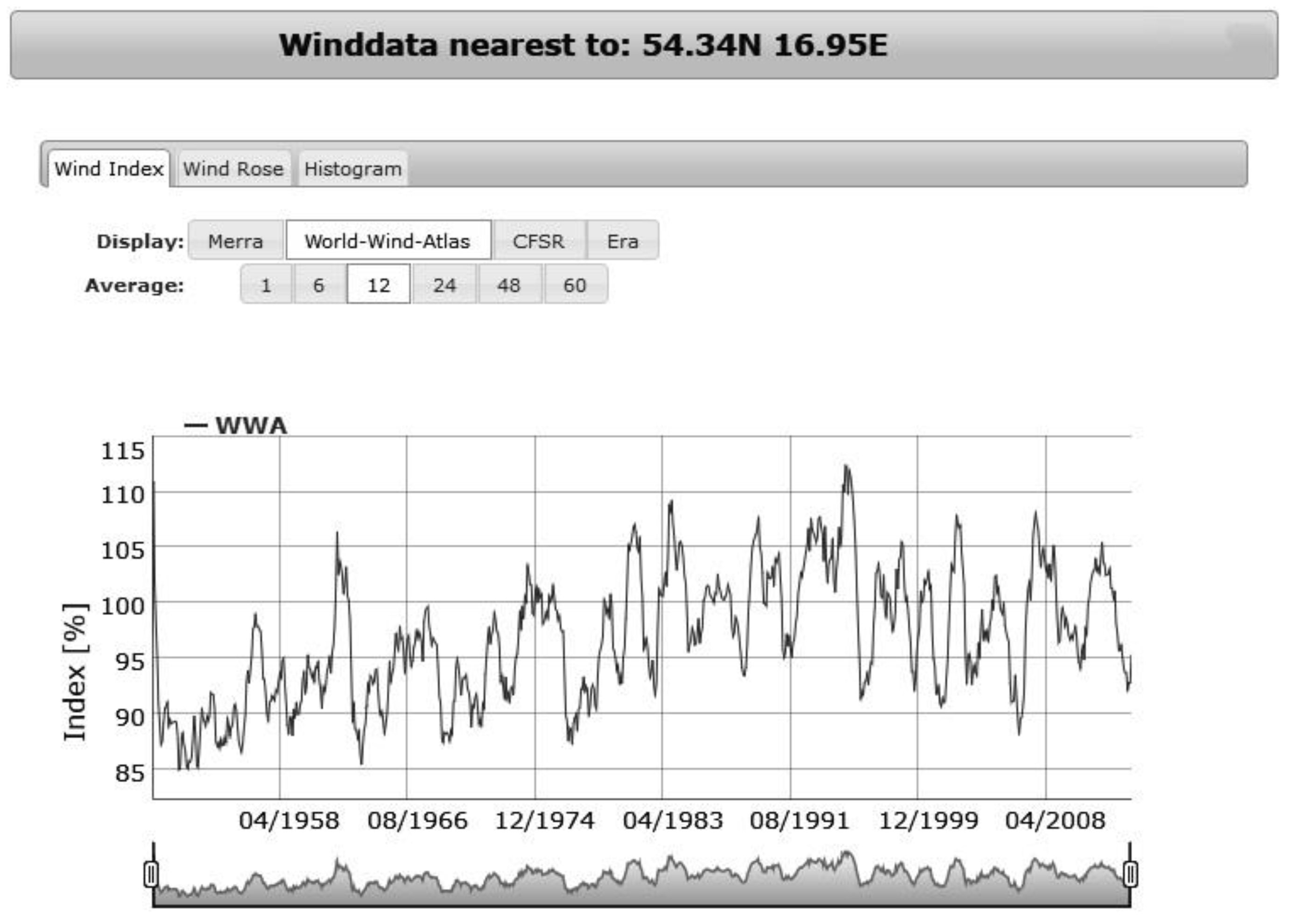
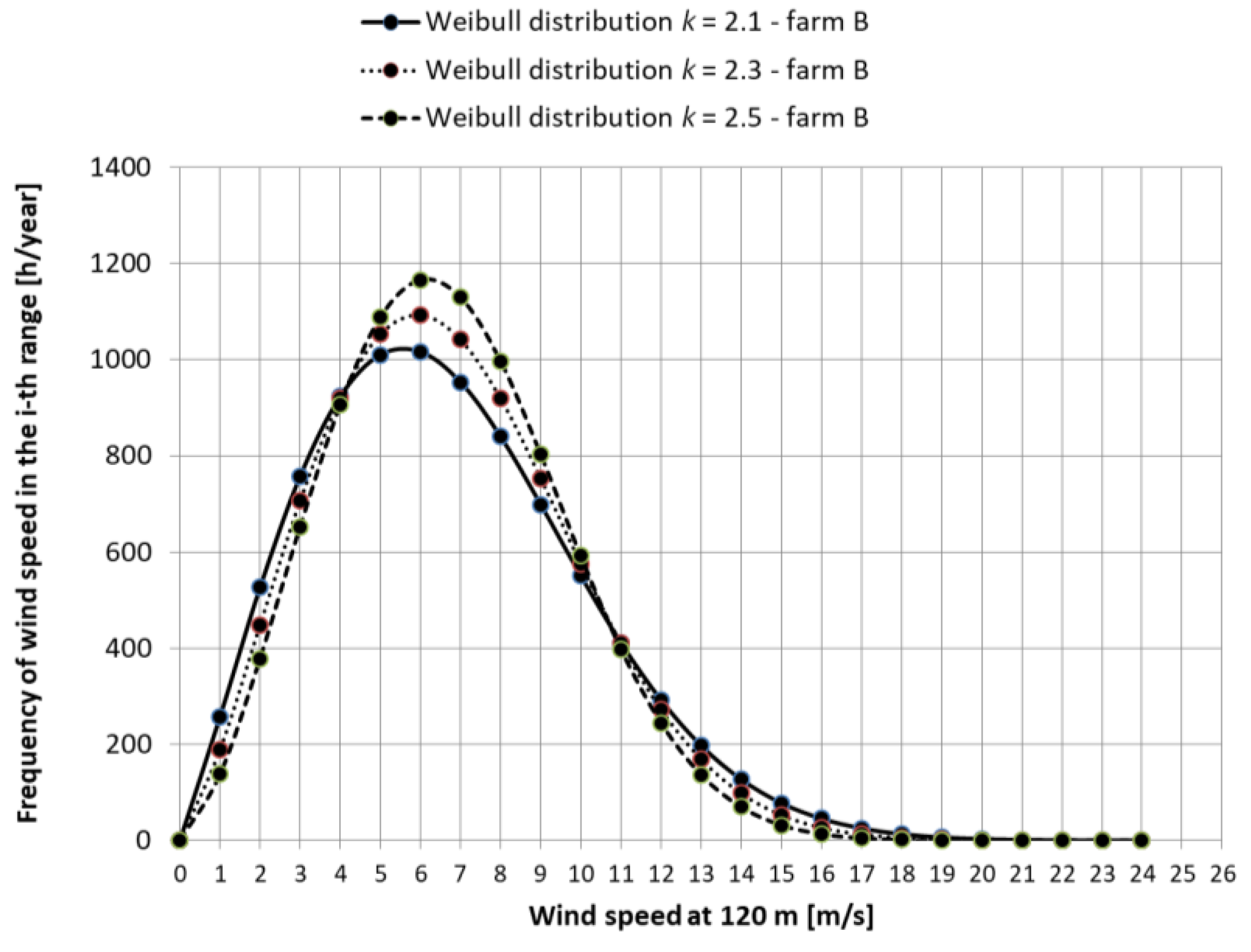
3.2. Wind Speed Distribution in Selected Locations

The following analysis used the results of the wind measurements performed in future locations for two wind farms in northern Poland. The two future farms are separated by a distance of over 100 km. Accuracy and correctness for the validation and analysis of measurement data are key determinants for the applicability of the given location in terms of its wind potential. The basic objective of the final report from wind measurements is the summary of the period of measurement and presentation of the results in graphic or tabular form. Construction of wind turbines with the tower height of 120 m above the ground was assumed. As a result of the performed measurement campaign, average wind speeds were obtained, listed in

Table 2. Wind speed results obtained from measurements.

Farm A		Farm B
Measuring Height, m	Wind Speed, m/s	Measuring Height, m	Wind Speed, m/s
35	495	30	493
65	579	58	576
98	644	60	583
100	658	-	-

.

Interaction between the terrain surface and air movement results in wind speed values varying with height. The vertical profile of wind speed is strongly linked to the land type. Flat areas produce lower wind disturbance than built-up areas [35,36,37]. In wind energy, the wind profile is typically explained according to the Equation (5) or (6):

$$\frac{v_1}{v_{ref}}={\left(\frac{h}{h_{ref}}\right)}^{\alpha }$$

(5)

$$\frac{v_1}{v_{ref}}=\frac{ln\left(\frac{h}{z_0}\right)}{ln\left(\frac{h_{ref}}{z_0}\right)}$$

(6)

After the Equation (5) was transformed, the α time exponent was calculated. After substitution of measurement data listed in Table 2, its mean value was determined

$$\alpha =\frac{log\frac{v}{v_{ref}}}{log\frac{h}{h_{ref}}}$$

(7)

for both locations. For farm A, α = 0.256 was obtained, whereas for farm B α = 0.237. Subsequently, average wind speed at h = 120 m was calculated with the use of Equation (5) for both locations. For farm A the average wind speed was v_1A = 6.79 m/s and v_1B = 6.87 m/s for farm B. The values of α exponent described for rural areas in the literature [35,38] range from 0.17 to 0.25. Value 0.25 concerns areas with low number of trees, suburbs of large cities, neighboring villages and undulating areas, which is in line with the actual state of both locations. By determining the mean wind speed with the use of Equation (6), we assumed z₀ = 0.25 m, which corresponds to a location near a village, rows of trees, scattered buildings and high cultivation areas [38]. The obtained average wind speed values at the height of 120 m were v_1A = 6.43 m/s for farm A and v_1B = 6.57 m/s for farm B. For further analyses average values from both estimations were assumed and the final average values were established at v_1A = 6.61 m/s and v_1B = 6.72 m/s.

Maximum heights of the wind measurements for both farms were lower than the planned height of wind turbine towers. Knowing the average wind speed at the desired height (120 m), the wind speed distribution was generated using two-parameter Weibull function. It must be noted that the provided parameters are a mathematical result. Though different wind speed distribution models are applied to fit the wind speed over a time period, the two-parameter Weibull function is accepted as the most popular technique [38].

The two-parameter Weibull probability density function is expressed by:

$$p\left(v\right)=\left(\frac{k}{A}\right){\left(\frac{v}{A}\right)}^{k-1}{e}^{-{\left(\frac{v}{A}\right)}^k}$$

(8)

where v, k, A > 0.

Dimensionless factor k determines the shape of the curve and is called a shape factor. Parameter A is the scale parameter. The distributions take different shapes with different values of k and A. Parameter k specifies the shape of a Weibull distribution and takes on a value of between 1 and 3. A small value for k signifies very variable winds, while constant winds are characterized by a larger k. Parameter A was calculated on the basis of the following relationship:

$$A=\frac{v}{\Gamma \left(1+\frac{1}{k}\right)}$$

(9)

With the wind speed distributions at the measured height (Table 2) being available, the Weibull distribution was adjusted to them. It was established that the k parameter shape ranges in both locations from 2.1 to 2.5. Further analysis was conducted for three k parameter values, that is: 2.1, 2.3 and 2.5. Figure 2 and Figure 3 show Weibull probability density function results for both locations.

Percentage results obtained from the probability density function were multiplied by 8760 (total number of hours per year) in each wind speed class. Thus, the number of hours per year for each speed class were obtained.

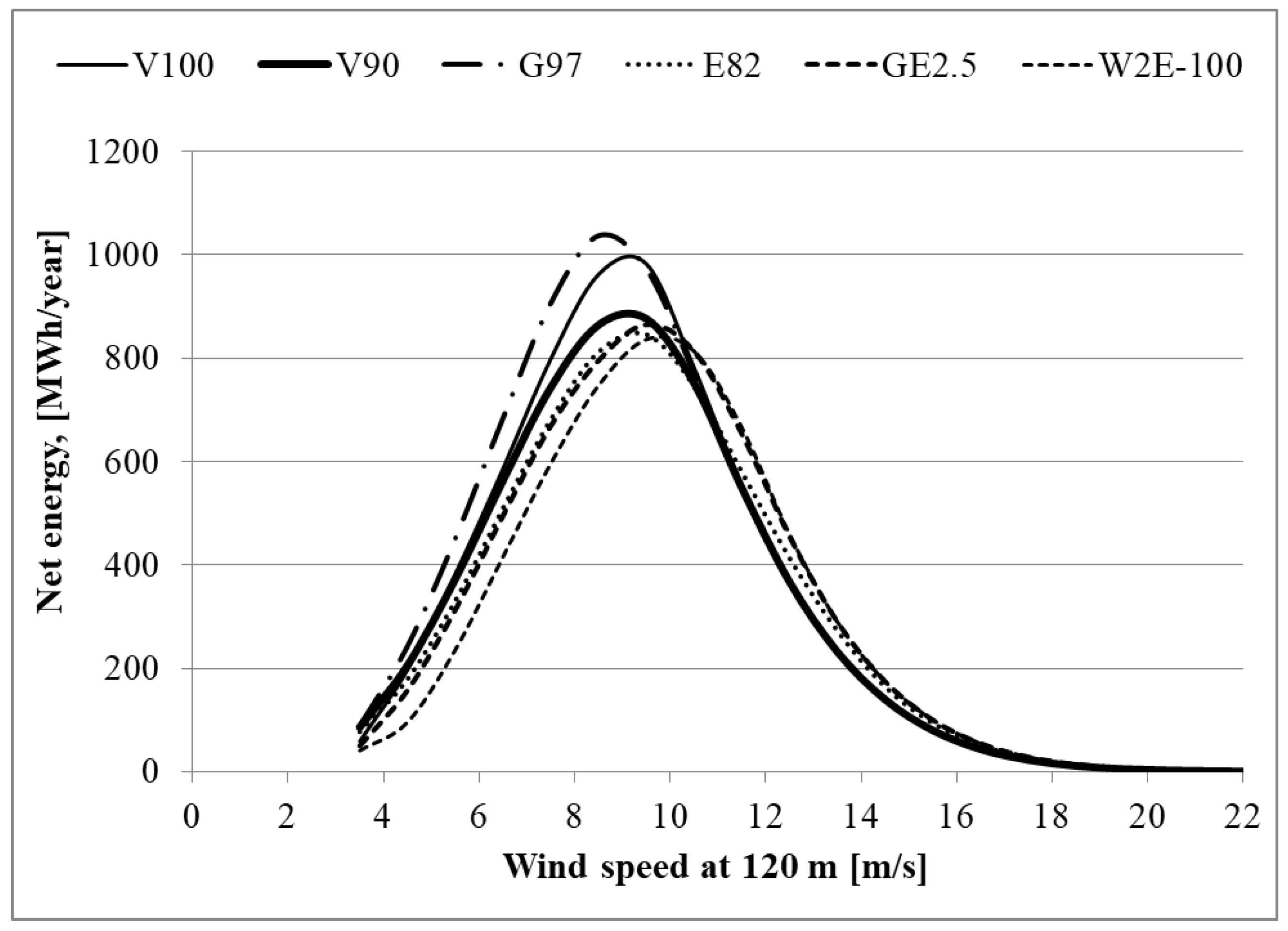
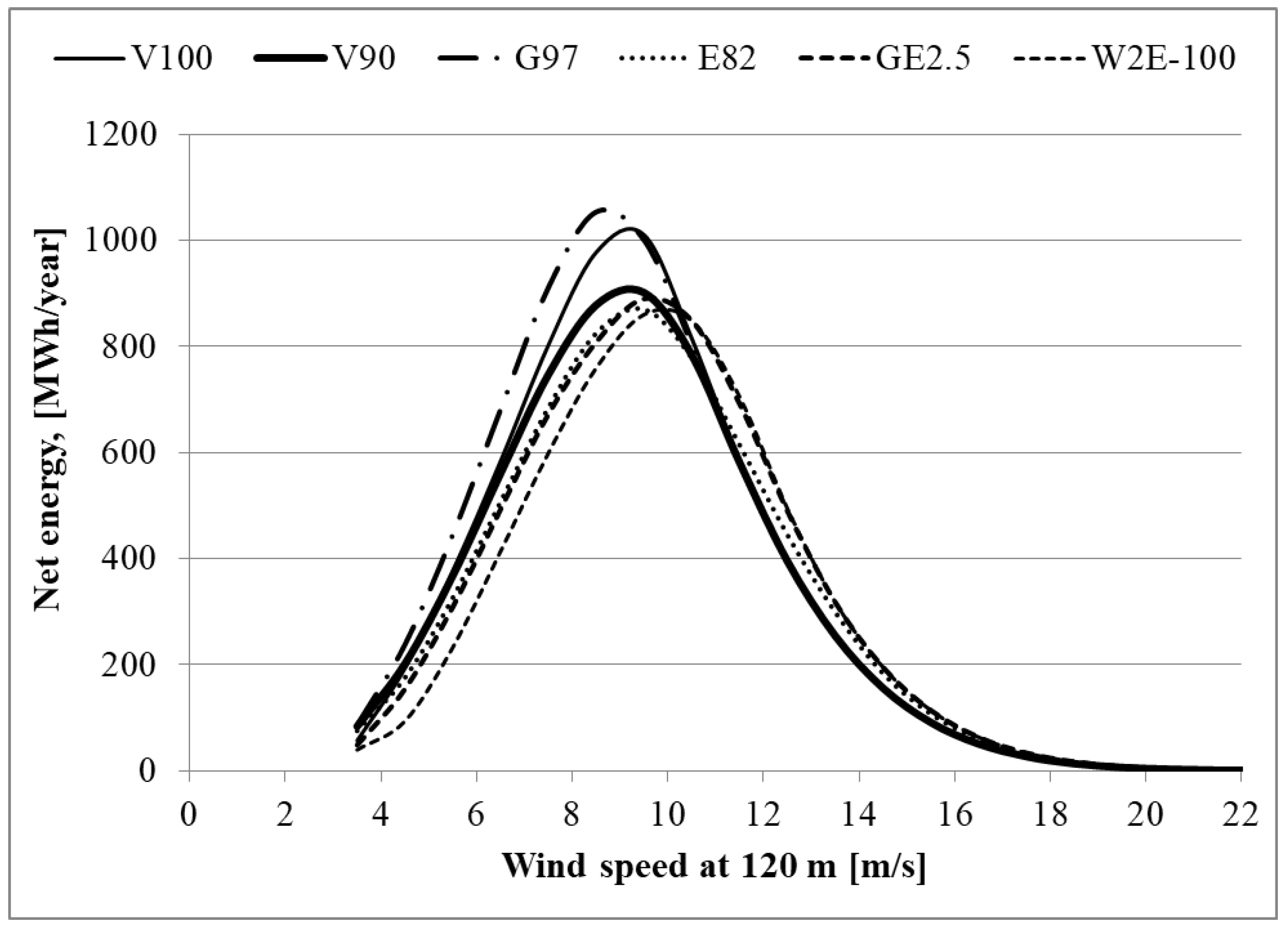
3.3. Wind Turbine Selection

Selection of wind turbine type and estimation of its energy performance for both locations was obtained based on the wind speed distribution histogram—Figure 2 and Figure 3. The calculations were performed considering the wind turbine characteristics provided by manufacturer, presenting the relationship between turbine power and wind speed—

Table 3. Wind turbines specifications.

Wind Speed, [m/s]	Power, [kW]
	V100	V90	G97	E82	GE2.5	W2E-100/2.55
0.50	-	-	-	-	-	-
1.50	-	-	-	-	-	-
2.50	-	-	-	-	-	-
3.50	62	91	94	82	53	43
4.50	192	200	236	174	153	93
5.50	371	362	438	321	304	229
6.50	612	588	714	532	517	434
7.50	955	889	1084	815	800	713
8.50	1398	1256	1507	1180	1156	1086
9.50	1835	1637	1817	1580	1616	1562
10.50	1980	1904	1951	1890	2061	2061
11.50	1999	1988	1990	2100	2366	2411
12.50	2000	1999	1998	2250	2477	2500
13.50	2000	2000	2000	2350	2498	2500
14.50	2000	2000	2000	2350	2500	2500
15.50	2000	2000	2000	2350	2500	2500
16.50	2000	2000	2000	2350	2500	2500
17.50	2000	2000	2000	2350	2500	2500
18.50	2000	2000	2000	2350	2500	2500
19.50	2000	2000	2000	2350	2500	2500
20.50	2000	2000	2000	2350	2500	2500
21.50	2000	2000	1906	2350	2500	2500
22.50	2000	2000	1681	2350	2500	2500

.

The available wind turbines power depends, among others, on the air density [38,39], which is a function of pressure and temperature—Equation (10).

$$\rho =\frac{p}{R T}$$

(10)

Change in the pressure with altitude can be presented with Equation (11).

$$p=101.29-0.011837\times h+4.793\times {10}^{-7}\times h^2$$

(11)

Based on the measurement data, it was determined that the temperature gradient in the studied locations is 0.5 K every 100 m, whereas air density in these locations is approximately ρ = 1.24 kg/m³. Unfortunately, wind turbine manufacturers rarely provide the performance of their devices for different air density values. Out of the selected range of turbines, only half were provided with such information. In the majority of devices, the power curve for air density ρ = 1.225 kg/m³ is presented. Not willing to restrict the analysis to three devices, further calculations were conducted for air density of ρ = 1.225 kg/m³.

Considering the Weibull distributions (Figure 2 and Figure 3) and the power curves of the selected turbines listed in Table 3, Figure 4, Figure 5, Figure 6, Figure 7, Figure 8 and Figure 9 show the distribution of the wind turbine performance in the studied locations for the different k parameters.

Figure 10 and Figure 11 list annual turbine performance for each location depending on k parameter value.

4. Results and Discussion

Analyses discussed in the Section 3 allowed obtaining data concerning the performance of the selected wind turbines. The G97 turbine turned out to be a clear leader in the studied locations. It generated the highest amount of energy that was supplied to the power grid, independently of the shape parameter k. The lowest productivity in the tested locations was demonstrated by the W2E-100 turbine. Figure 12 and Figure 13 demonstrate Weibull distribution and power production distribution, as well as power curves for the G97 and W2E-100 turbine. Data analysis indicates that the W2E-100 turbine attains its maximum power output at 13 m/s wind speed. This is considerably beyond the maximum power production capacity in the selected locations. The G97 attains the maximum power output for the wind speed of 11 m/s, which enables it to achieve higher performance.

Table 4. Energy performance coefficients.

Location	Performance Coefficient, [%]
	V100	V90	G97	E82	GE2.5	W2E-100/2.55
k = 2.1
Farm A	39.5	34.1	38.3	28.7	27.1	25.5
Farm B	40.4	35.0	39.2	29.5	28.2	26.5
k = 2.3
Farm A	39.6	33.9	38.3	28.1	26.5	24.7
Farm B	40.8	35.0	39.4	29.2	27.5	25.7
k = 2.5
Farm A	39.6	33.5	38.2	27.6	25.7	23.8
Farm B	40.8	34.7	39.4	28.6	26.9	25.0

lists performance coefficients of the analyzed wind turbines depending on the assumed k shape coefficient. The energy performance coefficient is the quotient of the actual annual production and the technically possible maximum energy production of a wind turbine. It should be noted that the wind turbines are not designed to maximize the energy performance coefficient, but rather to generate the highest possible power at determined wind speeds. Performance coefficients of 30–40% are considered very high in coastal areas.

The average cost of energy production for land wind turbines in 2017 was 60 $/MWh [2].

Table 5. Income generated by wind turbines.

Location	Income, [Thousand $]
	V100	V90	G97	E82	GE2.5	W2E-100/2.55
k = 2.1
Farm A	372	355	397	349	356	335
Farm B	384	367	408	348	370	348
k = 2.3
Farm A	371	352	397	342	348	324
Farm B	383	364	409	355	362	338
k = 2.5
Farm A	367	348	395	334	338	313
Farm B	381	361	409	348	353	328

lists annual income from energy production of the presented turbines depending on the assumed k shape coefficient.

The maximum difference between financial profit from G97, and W2E-100 amounted to 82,000$ per year. The difference in financial profit gained from energy production by these two wind turbines will reach 1,640,000$, while 20 years of their functioning.

And the maximum difference between financial profit from G97 and V100 is 28,000$ per year. In the period of 20 years, the income from the G97 turbine will increase by 560,000$. In this case, the winner is not as obvious. Purchase cost as well as service costs may be of significance when selecting the device.

The necessary specifications of the analyzed wind turbines were obtained from manufacturer technical specifications [40,41,42,43,44,45].

5. Conclusions

The present study demonstrated the manner in which wind turbine is selected on the basis of recorded annual wind measurements, with the emphasis on the obtaining the maximum financial benefits. The wind measurements demonstrated applicability of the tested locations in terms of their use as the construction site of a wind farm. Six types of wind turbines with different power outputs were tested. Turbines ensuring best usage of the wind energy resources in the studied locations have been indicated. Considering the hourly distribution of individual wind speeds, 2 MW turbines turned out to be the most energy efficient. The turbines with nominal power output of 2.3–2.5 MW demonstrated poorest performance in the tested locations.

The wind characteristics shall be analyzed for the site, where the wind turbine is to be located. Possible errors of performance estimation may stem from inaccurate prediction of the processed energy. In general, the wind measurements are performed at several heights, but typically below the height of the wind turbine boss. The calculation of the average wind speed value to a different height requires a precise analysis of the land topography. An incorrect assumption of the roughness index may result in overestimation or underestimation of the future wind farm performance.

The k Weibull shape coefficient has less pronounced impact on the distribution of individual wind speeds. At the same time, it has been demonstrated that a well selected wind turbine can be less sensitive to changes of the k coefficient. The analysis was performed on the basis of a one-year distribution of wind speed. It is a known fact that wind distribution will vary in time of wind turbines operation, and that it will oscillate around the multi-annual average value.

References

1. ECA. Wind and Solar Power for Electricity Generation: Significant Action Needed If EU Targets to be Met. Special Report No 08/2019; Publications Office of the European Union: Luxembourg, 2019. [Google Scholar]
2. Kuang, Y.; Zhang, Y.; Zhou, B.; Li, C.; Cao, Y.; Li, L.; Zeng, L. A review of renewable energy utilization in islands. Renew. Sustain. Energy Rev. 2016, 59, 504–513. [Google Scholar] [CrossRef]
3. Boczar, T. Wind Power. Current Potential; Measurement Automation and Monitoring: Gliwice, Poland, 2008. [Google Scholar]
4. U.S. EIA. International Energy Outlook 2019 with Projections to 2050; Office of Energy Analysis U.S. Department of Energy: Washington, DC, USA, 2019.
5. BP. BP Statistical Review of World Energy 2019, 68th ed.; Pureprint Group Limited: London, UK, 2019. [Google Scholar]
6. GWEC. Global Wind Statistics 2017; Global Wind Energy Council: Brussels, Belgium, 2018. [Google Scholar]
7. Kurpas, D.; Mroczek, B.; Karakiewicz, B.; Kassolik, K.; Andrzejewski, W. Health impact of wind farms. Ann. Agric. Environ. Med. 2013, 20, 595–605. [Google Scholar]
8. Letcher, T.M. Wind Energy Engineering: A Handbook for Onshore and Offshore Wind Turbines, 1st ed.; Academic Press: Cambridge, MA, USA; Elsevier: Amsterdam, The Netherlands, 2017. [Google Scholar]
9. Ehrlich, R.; Geller, H.A. Renewable Energy: A First Course, 2nd ed.; CRC Press: Boca Raton, FL, USA, 2018. [Google Scholar]
10. Drewitt, A.L.; Langston, R.H.W. Assessing the impact of wind farms on birds. Int. J. Avian Sci. 2006, 148, 29–42. [Google Scholar] [CrossRef]
11. Zagubień, A.; Ingielewicz, R. The analysis of similarity of calculation results and local measurements of wind farm noise. Measurement 2017, 106, 211–220. [Google Scholar] [CrossRef]
12. Zagubień, A.; Wolniewicz, K. The impact of supporting tower on wind turbine noise emission. Appl. Acoust. 2019, 5, 260–270. [Google Scholar] [CrossRef]
13. Liu, W.Y. A review on wind turbine noise mechanism and de-noising techniques. Renew. Energy 2017, 108, 311–320. [Google Scholar] [CrossRef]
14. Zagubień, A. Analysis of acoustic pressure fluctuation around wind farms. Pol. J. Environ. Stud. 2018, 27, 2843–2849. [Google Scholar] [CrossRef]
15. Celik, A. Energy output estimation for small scale wind power generators using Weibull representative wind data. J. Wind Eng. Ind. Aerodyn. 2003, 91, 693–707. [Google Scholar] [CrossRef]
16. Wais, P. Two and three-parameter Weibull distribution in available wind power analysis. Renew. Energy 2017, 103, 15–29. [Google Scholar] [CrossRef]
17. World-Wind-Atlas: 60+ Years Wind Data. Available online: https://sander-partner.com/en/products/wwa.html (accessed on 20 May 2021).
18. Jakubowski, M.; Mech, Ł.; Wolniewicz, K. A methodology of wind turbines selection for the given wind conditions. J. Mech. Energy Eng. 2017, 1, 171–178. [Google Scholar]
19. Emeksiz, C.; Cetin, T. In case study: Investigation of tower shadow disturbance and wind shear variations effects on energy production, wind speed and power characteristics. Sustain. Energy Technol. Assess. 2019, 35, 148–159. [Google Scholar] [CrossRef]
20. Wolniewicz, K.; Kuczyński, W.; Zagubień, A. Method for wind turbine selection basing on in-field measurements. J. Mech. Energy Eng. 2019, 3, 77–84. [Google Scholar] [CrossRef] [Green Version]
21. Wharton, S.; Lundquist, J.K. Assessing atmospheric stability and its impacts on rotor-disk wind characteristics at an onshore wind farm. Wind Energy 2012, 15, 525–546. [Google Scholar] [CrossRef]
22. IEC 61400-12-1:2005. Wind Turbines: Part 21-1: Power Performance of Electricity Producing Wind Turbines; IEC: Geneva, Switzerland, 2005. [Google Scholar]
23. Sanchez Gomez, M.; Lundquist, J. The effect of wind direction shear on turbine performance in a wind farm in central Iowa. Wind Energy Sci. Discuss. 2020, 5, 125–139. [Google Scholar] [CrossRef] [Green Version]
24. Jimoh, A.G.; Munda, J.L.; Agee, J. Wind distribution and capacity factor estimation for wind turbines in the coastal region of South Africa. Energy Convers. Manag. 2012, 64, 614–625. [Google Scholar] [CrossRef]
25. Adaramola, M.S.; Agelin-Chaab, M.; Paul, S.S. Assessment of wind power generation along the coast of Ghana. Energy Convers. Manag. 2014, 77, 61–69. [Google Scholar] [CrossRef]
26. Quan, P.; Thananchai, L. Assessment of wind energy potential for selecting wind turbines: An application to Thailand. Sustain. Energy Technol. Assess. 2015, 11, 17–26. [Google Scholar] [CrossRef]
27. Solangi, Y.; Tan, Q.; Waris, M.; Mirjat, N.; Ahmad, I. The Selection of Wind Power Project Location in the Southeastern Corridor of Pakistan: A Factor Analysis, AHP, and Fuzzy-TOPSIS Application. Energies 2018, 11, 1940. [Google Scholar] [CrossRef] [Green Version]
28. Zalewska, J.; Damaziak, K.; Malachowski, J. An Energy Efficiency Estimation Procedure for Small Wind Turbines at Chosen Locations in Poland. Energies 2021, 14, 3706. [Google Scholar] [CrossRef]
29. Yang, K. Geometry Design Optimization of a Wind Turbine Blade Considering Effects on Aerodynamic Performance by Linearization. Energies 2020, 13, 2320. [Google Scholar] [CrossRef]
30. Wolniewicz, K.; Zagubień, A.; Wesolowski, M. Energy and Acoustic Environmental Effective Approach for a Wind Farm Location. Energies 2021, 14, 7290. [Google Scholar] [CrossRef]
31. WWW.dtu.dk. Available online: https://windenergy.dtu.dk/english/research/publicationslist?dtulistcode=ISTLIST46&fr=1&mr=100&ptype=all&qt=DtuPublicationQuery (accessed on 27 October 2021).
32. Sedaghat, A.; Alkhatib, F.; Eilaghi, A.; Sabati, M.; Borvayeh, L.; Mostafaeipour, A. A new strategy for wind turbine selection using optimization based on rated wind speed. Energy Procedia 2019, 160, 582–589. [Google Scholar] [CrossRef]
33. Burton, T.; Sharoe, D.; Jenkins, N.; Bossanyi, E. Wind Energy Handbook; John Wiley & Sons Ltd.: Hoboken, NJ, USA, 2001. [Google Scholar] [CrossRef]
34. Manwell, J.F.; McGowan, J.G.; Rogers, A.L. Wind Energy Explained: Theory, Design and Application; Wiley: Hoboken, NJ, USA, 2009. [Google Scholar]
35. Wais, P. Wind Energy and Wind Turbine Selection. In Energy Science and Technology; Wind Energy; Studium Press LLC: Houston, TX, USA, 2015; Volume 8, pp. 168–193. [Google Scholar]
36. Bianchi, F.D.; de Battista, H.; Mantz, R.J. Wind Turbine Control Systems: Principles, Modelling and Gain Scheduling Design; Springer: London, UK, 2007. [Google Scholar]
37. Wu, X.; Hu, W.; Huang, Q.; Chen, C.; Chen, Z.; Blaabjerg, F. Optimized Placement of Onshore Wind Farms Considering Topography. Energies 2019, 12, 2944. [Google Scholar] [CrossRef] [Green Version]
38. Wais, P. A review of Weibull functions in wind sector. Renew. Sustain. Energy Rev. 2017, 70, 1099–1107. [Google Scholar] [CrossRef]
39. Jain, P. Wind Energy Engineering; McGraw-Hill: New York, NY, USA, 2010. [Google Scholar]
40. Vestas. Document No. 0062-4192 V01; VESTAS: Copenhagen, Denmark, 2018. [Google Scholar]
41. Vestas. Document No. 0062-4191 V04; VESTAS: Copenhagen, Denmark, 2017. [Google Scholar]
42. GE. Commercial Documentation Wind Turbine Generator Systems GE 2.5–100 m rotor 50 Hz & 60 Hz; GE: Fairfield, CT, USA, 2010. [Google Scholar]
43. W2E. General Description W2E-100/2.5; W2E: Rostock, German, 2008. [Google Scholar]
44. Enercon. Document No. SIAS-04-SPL E-82 E2 OM I 2.3 MW; Enercon: Berlin, German, 2010. [Google Scholar]
45. Gamesa. Document No. GD086484; Gamesa: Zamudio, Spain, 2010. [Google Scholar]
Figure 1. Multi-annual fluctuations of the mean of the wind speed (Farm A) [17].
Energies 14 07740 g001
Figure 2. The Weibull distribution for high at 120 m above ground level—farm A.
Energies 14 07740 g002
Figure 3. The Weibull distribution for high at 120 m above ground level—farm B.
Energies 14 07740 g003
Figure 4. Amount of the energy supplied to the power grid by the wind turbines as a function of the wind speed k = 2.1—farm A.
Energies 14 07740 g004
Figure 5. Amount of energy supplied to the power grid by the wind turbines as a function of the wind speed k = 2.3—farm A.
Energies 14 07740 g005
Figure 6. Amount of energy supplied to the power grid by the wind turbines as a function of the wind speed k = 2.5—farm A.
Energies 14 07740 g006
Figure 7. Amount of energy supplied to the power grid by the wind turbines as a function of the wind speed k = 2.1—farm B.
Energies 14 07740 g007
Figure 8. Amount of energy supplied to the power grid by the wind turbines as a function of the wind speed k = 2.3—farm B.
Energies 14 07740 g008
Figure 9. Amount of energy supplied to the power grid by the wind turbines as a function of the wind speed k = 2.5—farm B.
Energies 14 07740 g009
Figure 10. Amount of energy supplied to the power grid by the wind turbine—farm A.
Energies 14 07740 g010
Figure 11. Amount of energy supplied to the power grid by the wind turbine—farm B.
Energies 14 07740 g011
Figure 12. The power production distribution and the wind turbine power curves—farm A.
Energies 14 07740 g012
Figure 13. Power production distribution and wind turbine power curves—farm B.
Energies 14 07740 g013