A Study on a Floating Solar Energy System Applied in an Intertidal Zone

Abstract

This study was aimed at investigating a floating solar photovoltaic (FPV) system by numerical and experimental simulations under wave and wind loads to analyze the motion characteristics of the platform, the tension of the mooring line, and the pressure and uplift coefficient of panels at 2.5 m/5 m water depth conditions. The floating platform was installed with four rows of solar panels, each row with five panels, attached with four catenary types of mooring lines at the corner of the platform. The numerical model was based on ANSYS AQWA and ANSYS FLUENT (ANSYS Inc., Canonsburg, PA, USA). The experiment model was a scaled FPV platform with four rows of panels scaled in the 1:4 scale ratio. The results obtained from the experiment and numerical simulation achieved a good agreement. The results show that under normal sea conditions, the FPV system may resonate in a high frequency of wave condition, and a larger lift force occurred at the windward surface. Under extreme sea conditions, the pitch motion of the floating platform changed about ±6° without overturning; however, the wind will cause a large drift of the floating platform and the vortex area formed, which will cause damage to the solar panel.

1. Introduction

Renewable energy sources (RESs) have been increasing rapidly in recent years [1]. Globally RESs have registered an 8% yearly increase in installed power in the last 10 years [2]. This increase is being driven by the sensational development of the photovoltaic (PV) sector, which has registered a rate of growth of 45% [3]. The total solar PV installation capacity has reached 713 GW in 2020 [4]. As the available land area decreases, the market for land-based solar energy installations is gradually reaching saturation [5]. Floating solar photovoltaic (FPV) systems are now the mainstream form of electricity generation [6]. Most FPV systems are installed in enclosed water, such as lakes, ponds, reservoirs, etc. [7]. With the increase in energy demand, the concept of FPV systems established in near/offshore areas is proposed [1,7,8]. Therefore, floating solar energy has been the focus of many engineers and researchers these days [9,10]. There are several sites around the world with these systems installed, including in northern Europe, Latin America, China, Korea, Japan, etc. [11,12,13,14,15].

Unlike building in closed areas, installing an FPV system near shore encounters more technical difficulties [16]. Wave and wind effects, as well as water level changes, need to be considered [4]. Therefore, it is important to ensure the stability and safety of FPV systems under extreme sea conditions [17].

1.1. The Concepts of Different FPV Types

An FPV system consists of solar panels, floats, walkways, and float connections [4]. There is no unified standard for the type of floats. There are different designs from the manufacturing companies. The materials typically used for FPV systems are high-density polyethylene (HDPE), aluminum, carbon steel, and fiberglass with epoxy or polyester resin [4]. Various arrangements are designed for corresponding functional configurations. The most common FPV systems are classified into three types [3]. The first type uses HDPE pipes and steel or aluminum components to build rafts of large-scale systems, such as the Koine Multimedia by Terra Moretti. The second type is full HDPE rafts of mono-modules interconnected by suitable hooks, proposed by Ciel & Terre. The third type is floating pontoons interconnected, which is able to support the PV modules, and a typical example is the one developed by NRG Energy company (Houston, TX, USA).

1.2. Different Types of Mooring Systems

The mooring system used in the FPV system is divided into three categories—submerged mooring, shore mooring, and a hybrid of submerged and shore mooring [3]. The submerged mooring is divided into catenary mooring and taut leg mooring. The choice of mooring type depends on different environmental conditions, such as topography, soil condition, bathymetry, water space, and water level variation.

1.3. Environmental Condition in Intertidal Zone

Taiwan is located in the subtropical region and has plenty of sunshine, which is very suitable for developing solar energy sources. In order to effectively increase the use of solar energy, the government has promoted the Million Rooftop PVs Project since 2012 and listed the green energy industry as one of the five innovative industries. Most of the FPV system has been built in inland waters in Taiwan since 2016. The target site of this study is the 180 MW FPV plant, which is located in the intertidal zone water area (Figure 1). Normally, the wave is induced by local wind force, and the wave height range is about 0.1 to 0.4 m. The current factor was not considered in this study, as the embankment blocked the passage of current. In normal sea conditions, the water depth varies from 1.5 to 4 m due to the tide level variation. However, the water depth could reach 5 m under 50 return period consideration.

2. Materials and Methods

2.1. Numerical Simulation

First, we conducted a free decay and time response of FPV motion under wave and wind combined effect in AQWA [18]. Then, the floating platform angle motion of FPV investigated from AQWA was input in FLUENT [19] and analyzed the surface pressure of solar panels.

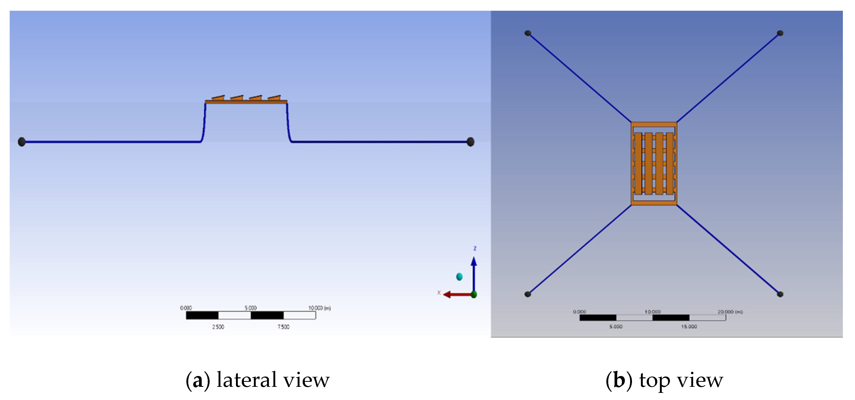
2.1.1. Numerical Setup

Herein, AQWA analyzes the diffraction and radiation effects of a floating system when subjected to wave loads. The hydrodynamic loads of AQWA are based on potential theory, which supposes that fluid is incompressible, inviscid, and irrotational flow. Under the assumptions of the open boundary water and the potential flow theory, the general equation of motion is

$$F\left(\omega \right)=M_s·\ddot{x}+M_a\left(\omega \right)·\ddot{x}+B\left(\omega \right)·\dot{x}+C·x,$$

(1)

where $M_s$ is structure mass, and $M_a$ is added mass (frequency dependent), $B$ is damping (frequency dependent), $C$ is hydrostatic stiffness, $F$ is wave force (incident and diffracting force), and $\dot{x}$ and $x$ are the velocity and displacement of the body.

For slender cylindrical elements whose element diameter divided by wavelength is less than 2, the hydrodynamic load can be calculated using the Morison equation as follows:

$$\begin{gathered} dF=\frac{1}{2}{\rho }_{w}D{C}_d\left|u_f-u_s\right|\left(u_f-u_s\right)+{\rho }_{w}A{C}_m{\dot{u}}_f-{\rho }_{w}A\left(C_m-1\right){\dot{u}}_s \\ =\frac{1}{2}{\rho }_{w}D{C}_d\left|u_f-u_s\right|\left(u_f-u_s\right)+{\rho }_{w}A\left(1+C_a\right){\dot{u}}_f-{\rho }_{w}A{C}_a{\dot{u}}_s, \end{gathered}$$

(2)

where ${\rho }_w$ is the density of water, $C_d$ is the drag coefficient, $D$ is the characteristic drag diameter, $u_{f },{\dot{u}}_f$ are the transverse directional fluid particle velocity and acceleration, $u_s,{\dot{u}}_s$ are the transverse directional structure velocity and acceleration, $C_m=C_a+1$ is the inertia coefficient, and $A$ is the cross-sectional area.

FLUENT is a computational fluid dynamics (CFD) software. It is used to simulate the surface pressure patterns of the solar panel under the action of wind. The 3D Reynolds-averaged Navier–Stokes simulations use a finite volume solver with a steady velocity inlet condition. The parameter of a reliable k-epsilon model with a first grid point of y⁺ ~30 was used herein [20,21]. The model with flows involving boundary layers under strong adverse pressure gradients, separation, and recirculation exhibits superior performance to the SST k-omega model [22]. The relationship between pressure and velocity was solved by a semi-implicit method for the pressure-linked equation (SIMPLE). The conservation equations were solved.

$$\frac{\partial {\rho }_a}{\partial t}+\nabla ·\left({\rho }_a\stackrel{\rightharpoonup }{u}\right)=0$$

(3)

$${\rho }_a\left(\frac{\partial \stackrel{\rightharpoonup }{u}}{\partial t}+\left(\stackrel{\rightharpoonup }{u}·\nabla \right)\stackrel{\rightharpoonup }{u}\right)=-\nabla p+\mu {\nabla }^2\stackrel{\rightharpoonup }{u}+f,$$

(4)

where ${\rho }_a$, u, p, μ, and f are the air density, the velocity component, the pressure, the dynamic viscosity, and other factors, respectively.

The realizable k-epsilon equations are shown as follows:

$$\frac{\partial \left({\rho }_{a}k\right)}{\partial t}+\frac{\partial \left({\rho }_{a}k{u}_j\right)}{\partial x_j}=\frac{\partial }{\partial x_j}\left[\left(\mu +\frac{{\mu }_t}{{\sigma }_k}\right)\frac{\partial k}{\partial x_j}\right]+G_k+G_b-{\rho }_a\epsilon -Y_M-S_k$$

(5)

$$\begin{gathered} \frac{\partial \left({\rho }_a\epsilon \right)}{\partial t}+\frac{\partial \left({\rho }_a\epsilon u_j\right)}{\partial x_j}=\frac{\partial }{\partial x_j}\left[\left(\mu +\frac{{\mu }_t}{{\sigma }_{\epsilon }}\right)\frac{\partial \epsilon }{\partial x_j}\right]+{\rho }_a{C}_l{S}_{\epsilon }-{\rho }_a{C}_2\frac{{\epsilon }^2}{k+\sqrt{\nu \epsilon }} \\ +C_{1\epsilon }\frac{\epsilon }{k}{C}_{3\epsilon }{G}_b+S_{\epsilon }, \end{gathered}$$

(6)

where

$$C_1=max\left(0.43\frac{\eta }{\eta +5}\right)$$

$$\eta =S\frac{k}{\epsilon }$$

$$S=\sqrt{{2S}_{ij}{S}_{ij}},$$

where G_k and G_b represent the generation of turbulence kinetic energy due to mean velocity gradients and buoyancy, respectively. Y_M is the contribution of the fluctuation dilatation in the compressible turbulence to the overall dissipation rate. σ_k and σ_ε are the turbulent Prandtl numbers for k and ε, while C₂ and C_1ε are constants. S_k and S_ε are user-defined source terms. The constants are σ_k = 1.0, σ_ε = 1.2, C_1ε = 1.44, and C₂ = 1.9.

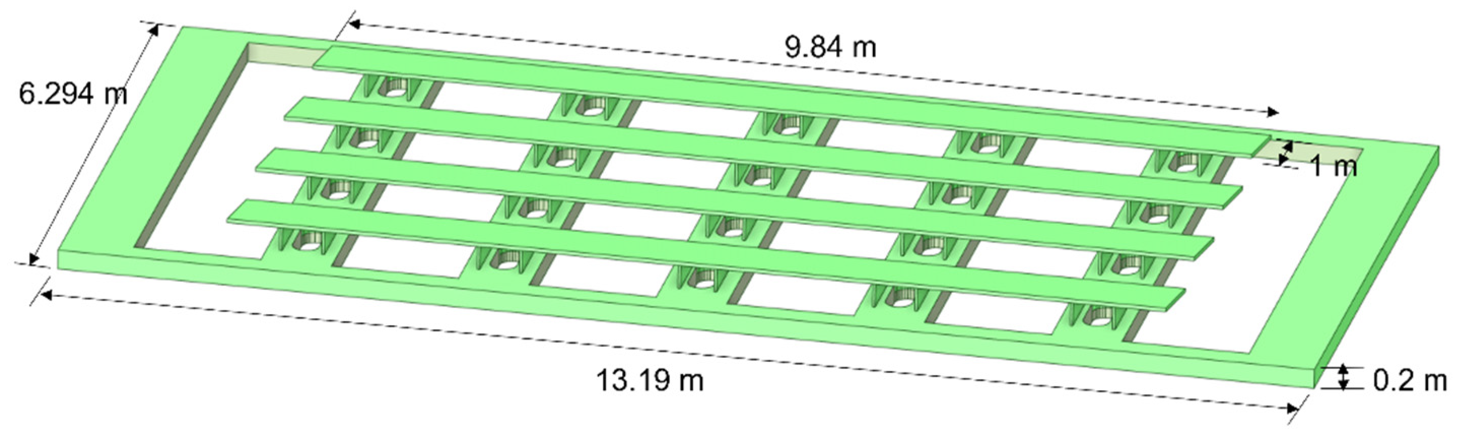
2.1.2. Model of the FPV System

The FPV model used in this study has 5 solar panels of 4 rows as an array module, as shown in Figure 2. The solar panel is 9.84 m long, 1 m wide, and 0.04 m thick. The floating platform is 13 m long, 6 m wide, and the tilt angle of the solar panel is 10°. Owing to the gap between adjacent panels being prone to eddy existing, each row of photovoltaic panels was combined into a complete long panel [23] in order to simplify the difficulty of numerical simulation. The detailed parameters are listed in

Table 1. Properties of FPV system.

FPV System Properties
Mass (kg)	3639.4
XCG (m)	0
YCG (m)	0
ZCG below sea level (m)	0
Roll inertia (kg·m2)	15,452
Pitch inertia (kg·m2)	65,646
Yaw inertia (kg·m2)	80,873
platform size (L × W × H) (m)	13.19 × 6.294 × 0.2
Panel size (L × w) (m)	9.84 × 0.992
Tilt angle (°)	10

. The XCG, YCG, and ZCG are the gravity center coordination related to the water surface.

A mooring system was used to keep the floating platform within a specified range, and it would provide the floating platform stability. The catenary type of mooring line was adopted in this study (Figure 3), and the main consideration was the change of water level in the intertidal zone. The reference site is located in the intertidal zone within water depth from 2.5 m to 5 m due to tidal variation in midwestern Taiwan. The floating platform’s range of motion with the wave motion can be determined by the suspended mooring type. Furthermore, the mooring line cannot easily break due to the snap load that causes the cable to generate great tension [24]. According to these considerations, the mooring line material was designed as the R4 chain, and the length of the chain was 22 m. The weight per unit length in the air was chosen as 27.88 kg/m, and the chain diameter was 0.04 m. The detailed information is shown in

Table 2. Properties of mooring system.

Mooring Properties of FPV System
Diameter (m)	0.04
Unit weight (kg/m)	27.88
Number of mooring lines	4
Unstretched mooring line length (m)	22
Breaking load (kN)	1788.67
Stiffness (kN)	136,640

.

Figure 4 shows the computational domain and grid built by Mesh, which is a function used in FLUENT. The location of the FPV model was in a computational domain with a spatial dimension of 15 L (length) × 5 L (width) × 10 L (height), with an upstream fetch of 5 L and a downstream length of 10 L. L is the characteristic length of the floating platform. The wind velocity at the inlet was 6 m/s above water level, with 1.0 m in height. There were stationary, no-slip, non-penetrating, and adiabatic sidewalls. Moving upper and lower walls, corresponding to variation in the tilt angle of the solar panel, were used by moving grids. The numerical meshes were determined by using a grid sensitivity study for grids of 10 million cells.

2.2. Experimental Setup

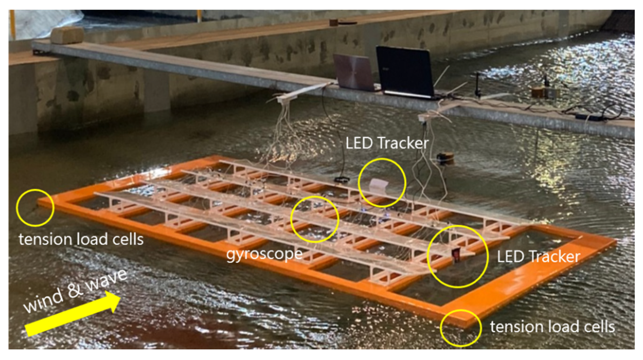
2.2.1. Experiment Model

The 1/4 scaled model was made of integral skin-foam sheets, the bracket and the photoelectric panel frame were made of acrylic material, and the photoelectric panel was a transparent plastic soft board (Figure 5).

With an aim to achieve the same restoring force to numerical simulation in the experiment, the mooring system was scaled with chain and spring, and the stiffness must be in accordance with the catenary equation (Figure 6). The chain nominal diameter of the designed mooring system was 7 mm. A Grade R4 stud-less chain was chosen as the mooring component. The unstretched mooring line length was 2 m.

2.2.2. Wave/Wind/Current Basin and Instrumentation

The experiment was conducted in wave/wind/current basin in Tainan Hydraulics Laboratory (THL) in National Cheng Kung University (NCKU) (Figure 7). The basin is 60 m long, 7 m wide, and 1.2 m deep, and equipped with long crest wave generators operating through an electro control system producing irregular waves up to 0.32 m high at T_peak of 1.6 to 2.5 s. Figure 8 shows the location of the sensors on the FPV model system. Three capacitance wave gauges were used to measure the wave elevations during the model test. LED system was installed to track the heave and surge motion of the platform. The gyroscope, which was manufactured by XSENS, Enschede, Netherlands, was used to measure the accelerations and rotations of the 3 axes of the platform. Two tension load cells, which were manufactured by SSK, Japan, were installed on the fairlead of the platform to measure the mooring line tension.

In the hydraulic model test and the wind tunnel test, the Froude number and the Reynolds number had to be considered. Due to the scale effect between Reynolds number and Froude number, the scaled model could not satisfy the similarity of the two parameters at the same time. The lift coefficient and Reynolds number of solar photovoltaic panels are independent [25], which means that changes in wind speed do not affect the wind pressure coefficient (C_p) of photovoltaic panels. Therefore, in this study, a larger scale (1:4) model based on Reynolds number was used to reduce the difference of scale effect caused by the scale model’s extremely small size.

2.2.3. Irregular Wave Test

The numerical and experimental tests included the free decay and irregular wave and wind coupling tests. By the free decay test, we obtained the natural period of the FPV system. Then, the natural period was set as wave period in normal conditions with wave height in 0.2 m, and the wind speed was 6 m/s. The extreme case for intertidal zone wave condition under typhoon attack was determined from the result of the harbor sheltering model test by THL (2006). Thus, the wave height was 0.75 m, and the wave period was 8 s with the JONSWAP spectrum (peak ratio is 2.08), and the wind speed was 25 m/s.

Table 3. Test conditions of irregular waves and wind directions.

Case Name	Water Depth (m)	Wave Condition			Wind Condition
		Wave Height (m)	Wave Period (s)	Wave Direction (°)	Wind Speed (m/s)	Wind Direction (°)
JH020T1.4W6 (normal conditions)	2.5	0.20	1.4	0	6	0
				45		45
				90		90
				135		135
				180		180
JH075T8W25 (extreme conditions)	5	0.75	8	0	25	0
						90
						180

shows the irregular wave and wind conditions. The experiment was conducted only under the case of 0° for wave and wind directions under normal sea conditions due to the limited space of the basin.

Figure 9 is a schematic diagram of different wave directions (γ) and wind directions (β) under normal sea conditions and extreme sea conditions. In normal sea conditions, the waves and winds act in the same direction, while in extreme sea conditions, the wave direction is fixed, and the wind directions are 0°, 90°, and 180°.

3. Results and Discussion

The dynamic of wave and wind effect was fully investigated by ANSYS AQWA/FLUENT. The numerical results include the response of platform motion, mooring tensions, and the surface pressure/uplift coefficients of solar panels under wave and wind combined effect. Furthermore, the numerical result of platform motion and mooring force were compared with experimental results.

3.1. Free Decay Test

Figure 10 shows the free decay results of the numerical and experiment of the platform in heave, roll, and pitch without a mooring system.

Table 4. The comparison of natural period results between experiment and AQWA.

Natural Period	Heave	Roll	Pitch
Experiment	1.1 s	2.0 s	0.5 (1.4) s
AQWA	1.0 s	1.0 s	1.4 s

shows the comparison of the natural period results between the experiment and AQWA. In the numerical test, the natural period corresponding to the direction of heave, roll, and pitch were 1.0 s, 1.0 s, and 1.4 s, respectively. In the experiment’s test, the natural period corresponding to the direction of heave, roll, and pitch were 1.1 s, 2 s, and 0.5 s, respectively. However, there was another peak that occurred in 1.4 s (0.7 Hz) in the pitch direction. The reason was that the water in the damping pool of the floating platform also had a resonance period when the floating platform was in pitch/roll motion, which cannot be investigated by AQWA. However, the experimental result was similar to that of the experiment of Chuang et al. (2021). It is worth noting that three degrees of freedom of natural period are high-frequency wave conditions, which means that the FPV system has resonance in high-frequency ocean environments.

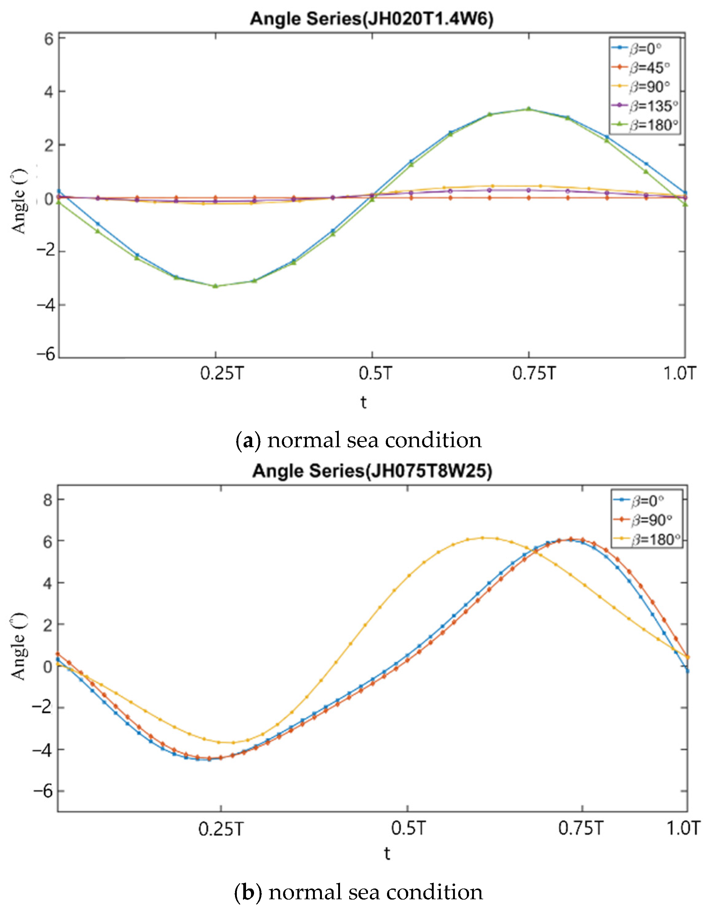
3.2. Irregular Wave Analysis from AQWA

Figure 11 shows the motion trajectory of the floating platform under normal sea conditions and extreme sea conditions. It was concentrated in a single direction when the wave and wind directions were 0°, 90°, and 180°. When the wave and wind directions were 45° and 135°, the moving area of the floating platform was about 2 m². When the wave wind angle was 90°, the platform moved close to the y-direction about 0.2 m, and the moving area was about 0.9 m². There was a maximum moving range of about 4.1 m when the wave and wind directions were 0°.

Figure 12, Figure 13 and Figure 14 are time series of the surge, heave, and pitch motions of the floating platform under normal sea conditions and extreme sea conditions. In normal sea conditions, the average response amplitude in the surge was almost the same, but different phases were presented with the change in wave and wind directions. There was a maximum response amplitude in heave and pitch when wave and wind directions were 0°, and it decreased as the wind direction changed from 0° to 180°. In normal sea conditions, the platform in different wave directions was about 1 m for surge amplitude, ±0.03 m for heave motion, and ±2° for pitch motion.

In extreme sea conditions, the wave direction was fixed, and the wind direction changed. There was a maximum response amplitude in the surge when wave and wind directions were 0°. However, the heave and pitch motions were the same despite the change in wind direction. In extreme sea conditions, the platform in different wind directions was up to 2 m for surge amplitude, ±0.5 m for heave motion on average, and ±5° for pitch motion on average.

Figure 15, Figure 16 and Figure 17 and

Table 5. The statistics of surge, heave, and pitch motions of platform in different cases.

	Normal Sea Condition			Extreme Sea Condition
	Surge	Heave	Pitch	Surge	Heave	Pitch
Mean	1.31 m	0 m	−0.04°	0.1 m	0 m	−0.04°
Standard deviation	0.38 m	0 m	0.64°	0.62 m	0.18 m	1.82°

show the statistical distributions of the platform in normal sea conditions and extreme sea conditions. In order to find the motion characteristics of the platform, we transferred the time series data into statistical distribution for surge, heave, and pitch data. It can be observed that the concentration ranges of FPV motion under normal sea conditions were within 0.93–1.68 m in the surge motion, ±0.01 m in heave, and ±0.6° for the pitch angle. However, the concentration ranges of FPV motion under extreme sea conditions were within −0.6–0.7 m in the surge motion, ±0.17 m in heave, and ±1.8° for the pitch angle. The results show that the distribution of motion under normal sea conditions was more concentrated than in extreme sea conditions. Under extreme sea conditions, the standard deviations of motion of floating platform in the surge, heave, and pitch directions were all greater than that of normal sea conditions. This indicates that the floating platform had greater motion behavior under extreme sea conditions, and the average value in the surge motion shows that the floating platform was concentrated at a position far from the origin under normal sea conditions, and it was a periodic motion through the origin under extreme sea conditions.

3.3. Tension Analysis from AQWA

Figure 18 and Figure 19 show the time series of the mooring line tension of the floating platform under normal sea conditions. It was found that the average tension of the mooring line in different wave directions ranged from 0.45 to 0.77 kN. It was interesting that the peak tension reached 9.81 kN, near computational time 1250 s. At the same time, the floating platform also had a high peak in surge and pitch motions. From this, it can be inferred that the instantaneous value of tension occurred because the wave condition was the resonance frequency of the floating platform. Therefore, the floating platform had a large response of surge and pitch motions that caused the mooring line to pull the floating platform instantaneously. The average tension of different wind directions ranged from 2.34 to 2.36 kN, indicating that the change in wind direction did not affect the mooring line tension, and there was no instantaneous extreme tension in extreme sea conditions.

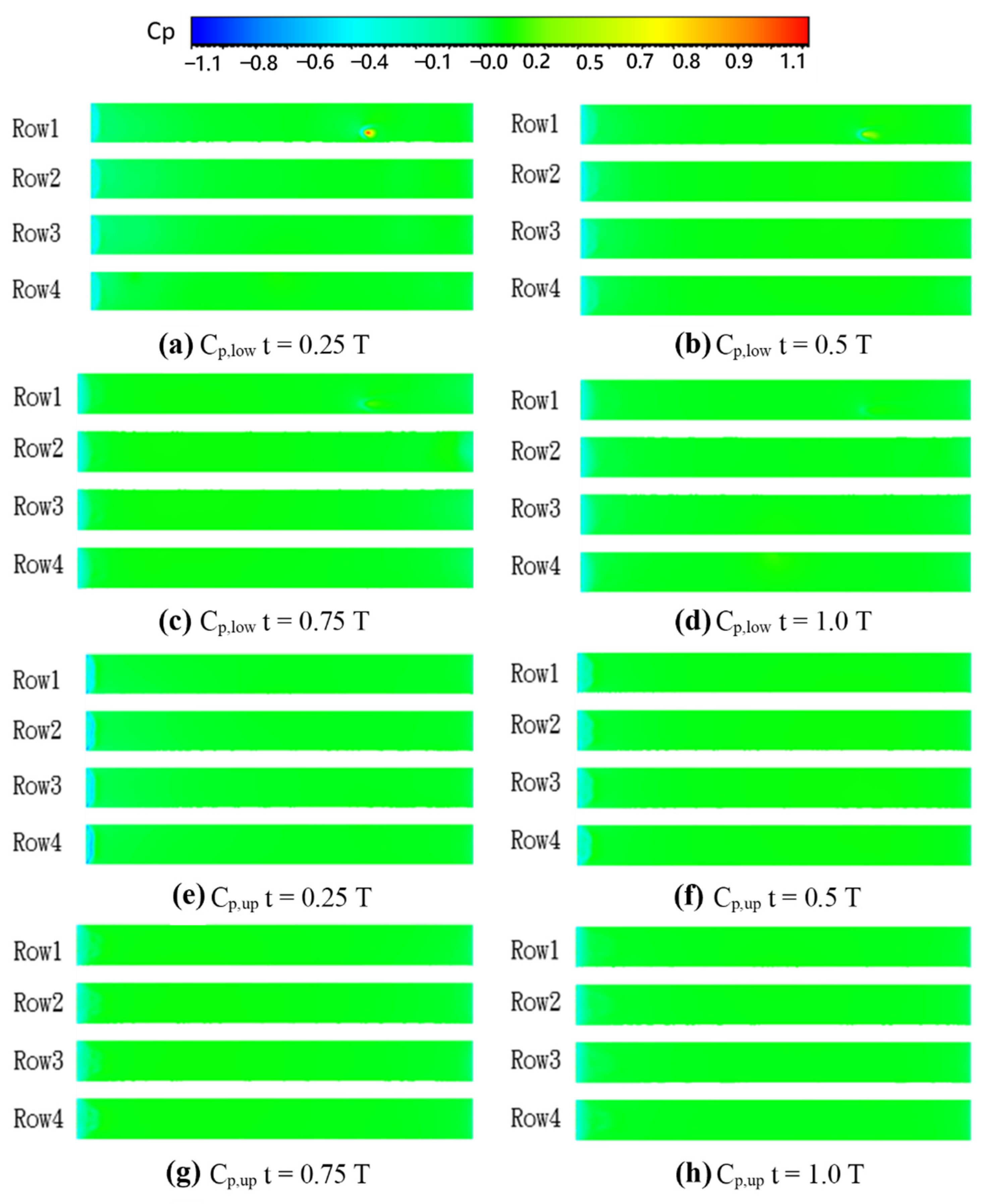
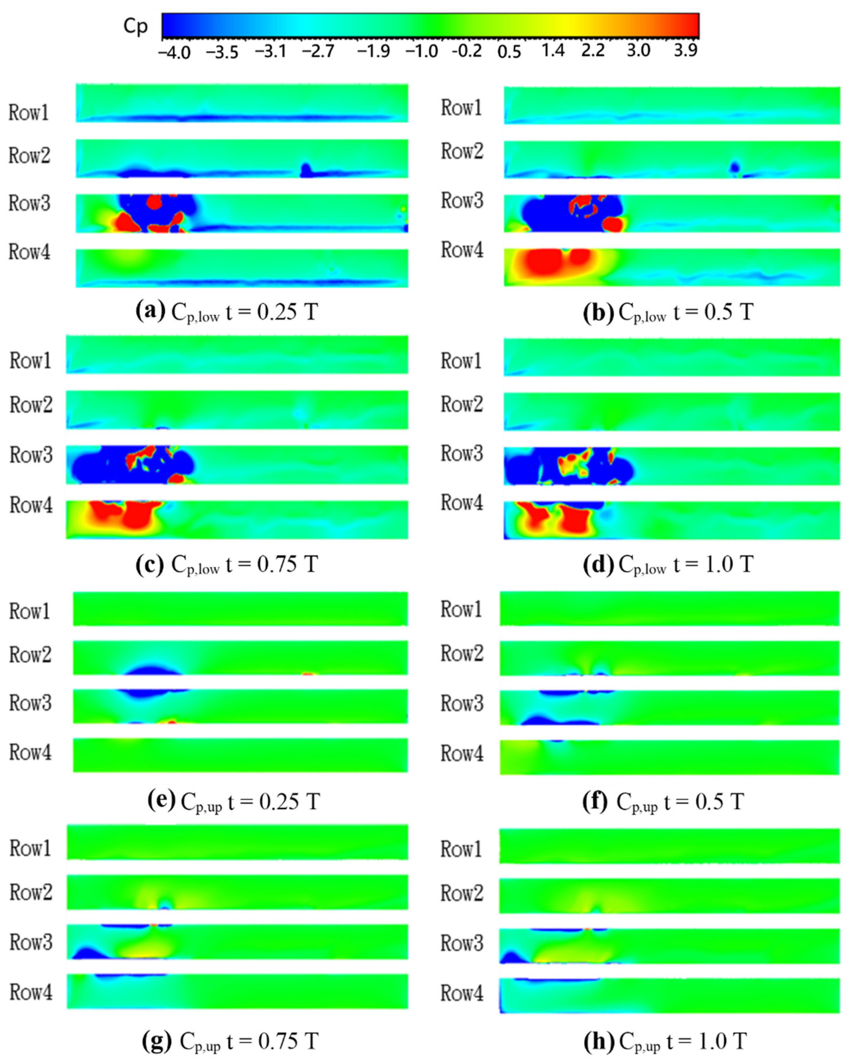
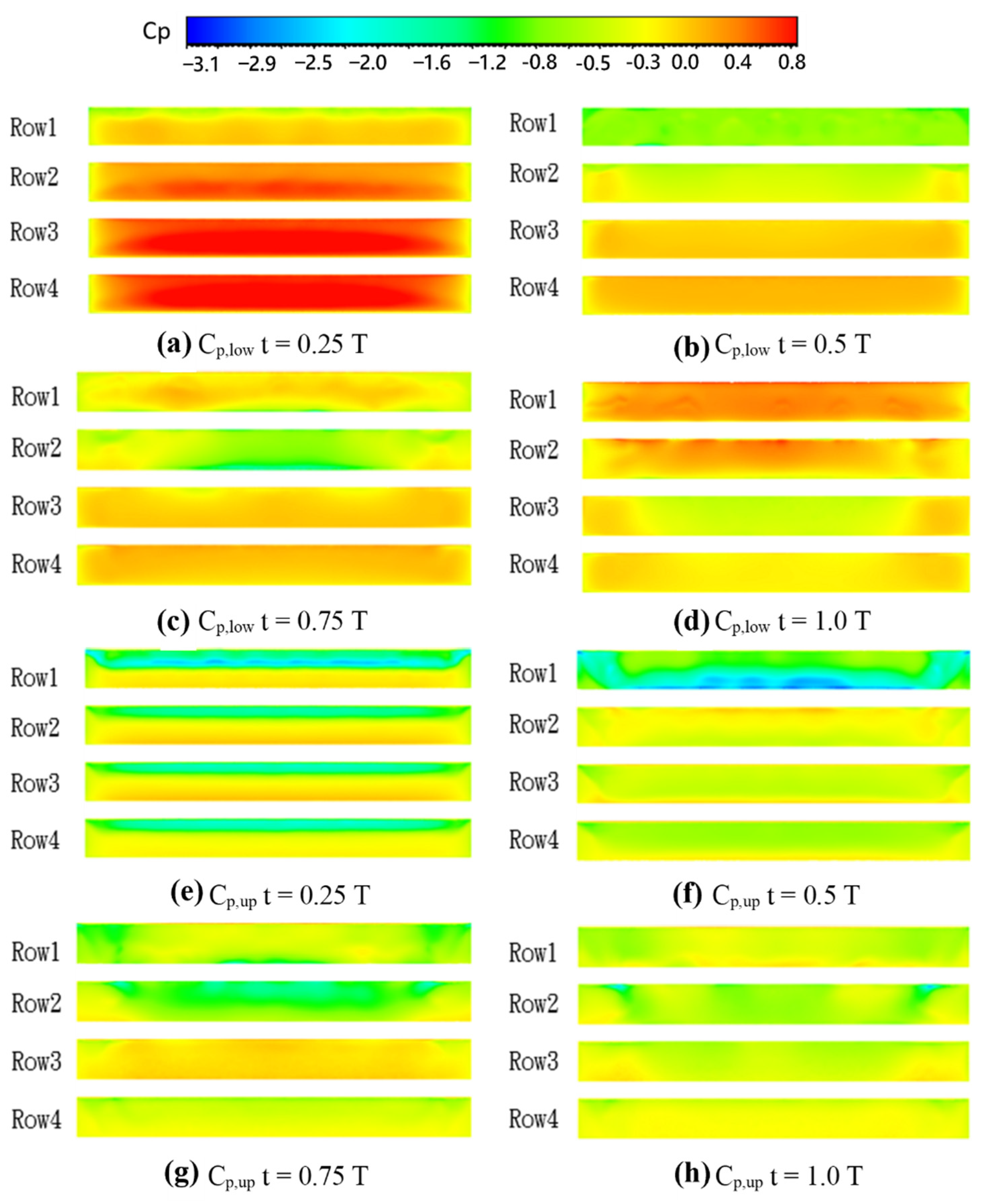
3.4. Pressure Coefficient from FLUENT

Figure 20 shows the maximum angle changes diagram of each case under the different stages of wave period (0.25T, 0.5T, 0.75T, 1.0T). According to this condition, the pressure coefficient, C_p on the upper and lower panels was analyzed, using Equation (7) as follows:

$$C_p=\frac{p-p_{\infty }}{q},$$

(7)

where $p_{\infty }$ is freestream static pressure; q is dynamic pressure.

Figure 21, Figure 22, Figure 23, Figure 24 and Figure 25 are the pressure coefficient patterns of the upper and lower surfaces with γ and β from 0° to 180° under normal sea conditions. When γ = 0° and β = 0°, the lower surface of row 1 was the windward surface. C_p in the middle of the lower surface was positive value, and the left and right sides were negative value due to the side-edge vortices form. The value of C_p was negative near the front edge on the upper surface because of the suction from flow separation. When the period stage changed, the positive value of C_p on the lower surfaces gradually decreased. It can be observed that the difference of pressure distribution on row 2 to row 4 of panels was not obvious due to the shadowing effect. When γ = 45° and β = 45°, C_p distribution slightly shifted near the windward corner with the wind direction.

When γ = 90° and β = 90°, there was almost no pressure on all surfaces under different period stages because the panel was parallel to the wind direction. When γ = 135° and β = 135°, row 3 and row 4 were the windward panels. There was a greater corner vortex near the lower and upper surfaces on row 3 and row 4. When γ = 180° and β = 180°, the upper surface of row 4 was the windward surface. As the angle variation of the panel was small, the value of C_p on the upper surface was not obvious when the period stage changed. There were negative values of C_p near the front edge of the lower surface of each row.

Figure 26, Figure 27 and Figure 28 are the pressure coefficient patterns of the upper and lower surfaces with γ = 0° and β = 0°, 90°, and 180° under extreme sea conditions. The result of pressure distribution under extreme sea conditions was similar to that of normal sea conditions.

3.5. Lift Coefficient from Fluent

The lift coefficient of the solar panel was calculated by integrating the differential pressure between upper and lower surfaces, using Equation (8) as follows:

$$C_L={\displaystyle \int }\left(C_{p,up}-C_{p,low}\right)cos\alpha dA,$$

(8)

where α is the tilt angle of the solar panel, and A is the area of the panel.

Figure 29, Figure 30, Figure 31, Figure 32 and Figure 33 depict the lift coefficient diagrams of the array solar panels under normal sea conditions. The results reveal that the solar panel had the maximum lift force at t = 0.25T, and the lift coefficient gradually increased with the increase in the period stage. Figure 29 shows that when β = 0°, γ = 0° and the period stage was at 0.25T, each row had the largest lift force. Row 4 had a higher lift force than the rest, and the lift force gradually decreased with the period stage. When the wind direction increased, the lift coefficient gradually increased, and the lift force gradually decreased, until the lift force of each row of panels was almost zero when β = 90°. When β > 90°, the surface of each row would gradually turn to bear downward pressure load. It is worth noting that when β = 135°, there was a recirculation zone between row 3 and row 4 of the lower surface, which caused the lift coefficient to change greatly. When β = 180°, the lift coefficient of each row of the panel was positive. Meanwhile, the panel was under clearly downward pressure, and the lift coefficient was greater than the value of the other wave period at 0.25T. Generally speaking, the simulation results show that the lift coefficient decreased when the wave and wind directions increased under normal sea conditions, and the maximum lift force occurred when β = 0° and γ = 0°, and the period stage was at 0.25T.

Figure 34, Figure 35 and Figure 36 display the graphs of the lift coefficients of solar panel arrays under extreme sea conditions. The distribution of lift coefficients had the same trend as that of normal sea conditions. When γ = 0° and β = 0°, the pitch angle of the solar panels was larger than those of normal sea conditions. In general, the lift coefficient increased as the period stage increased. When γ = 0°, β = 90°, the panel was parallel to the wind direction, and the value of C_L was almost zero of each row of surfaces. When γ = 0°, β = 180°, there was a large lift coefficient changed with row 4, while the remaining rows of panels had no obvious changes due to the shielding effect. At this time, each row of panels had a downward pressure at different stages of wave period.

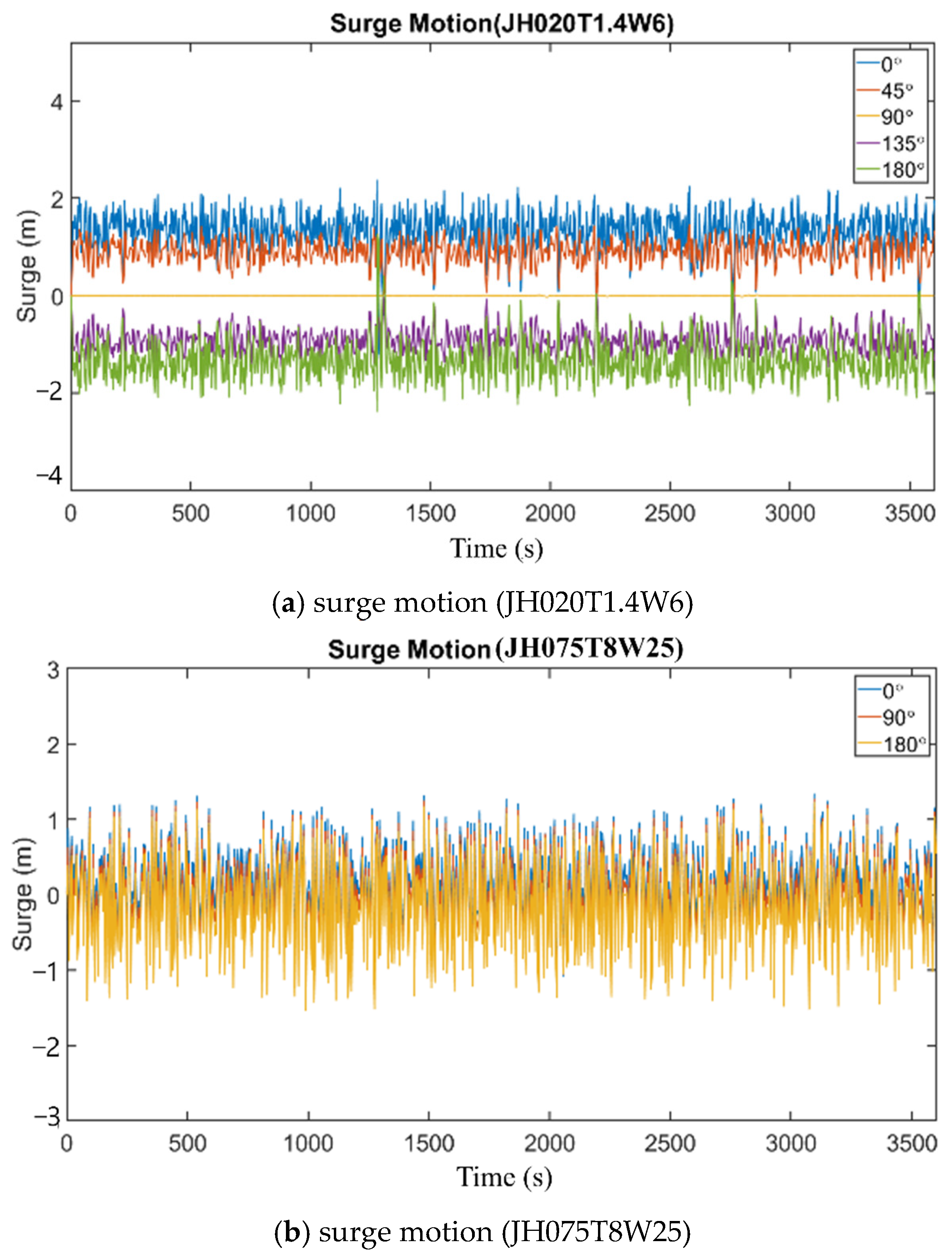
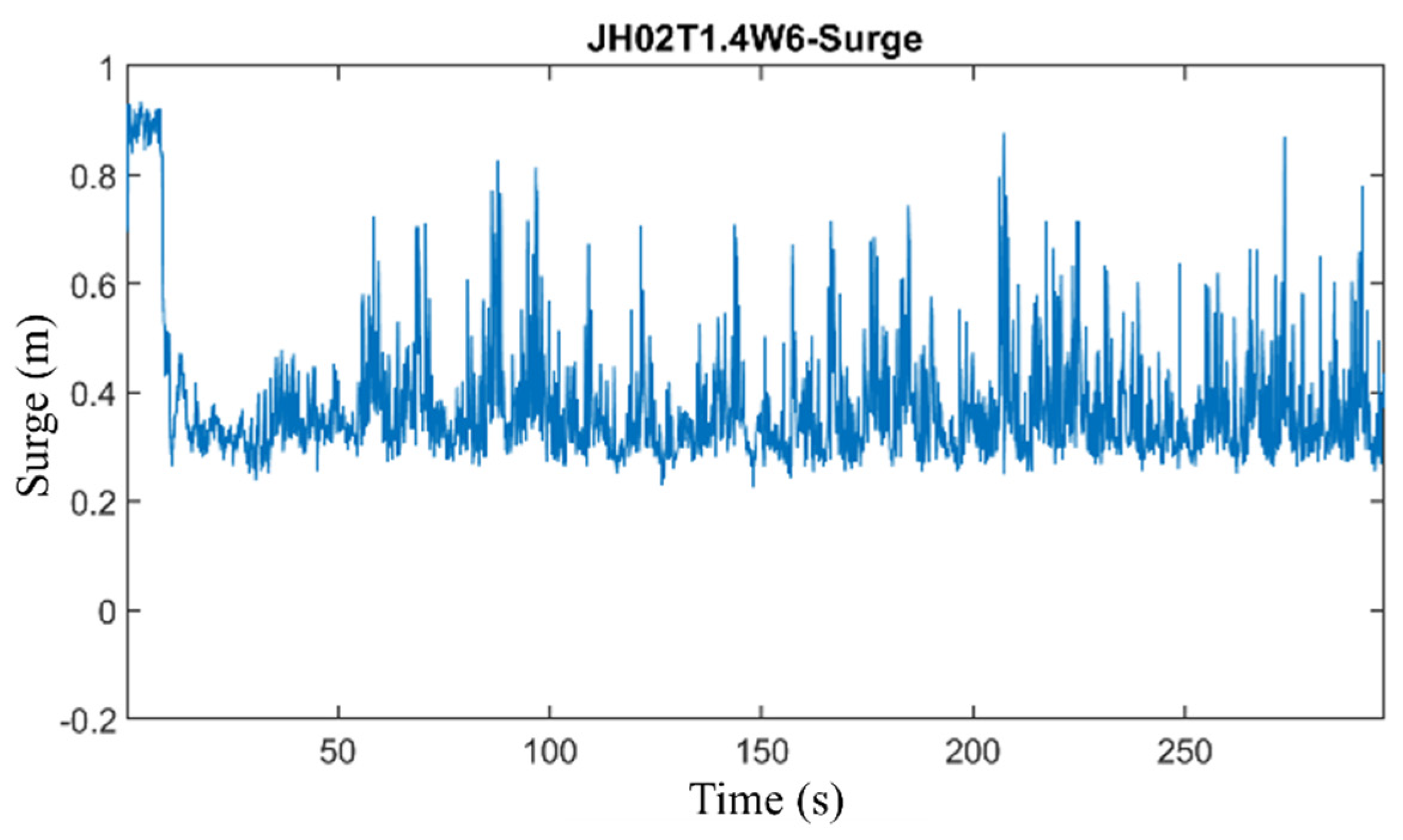
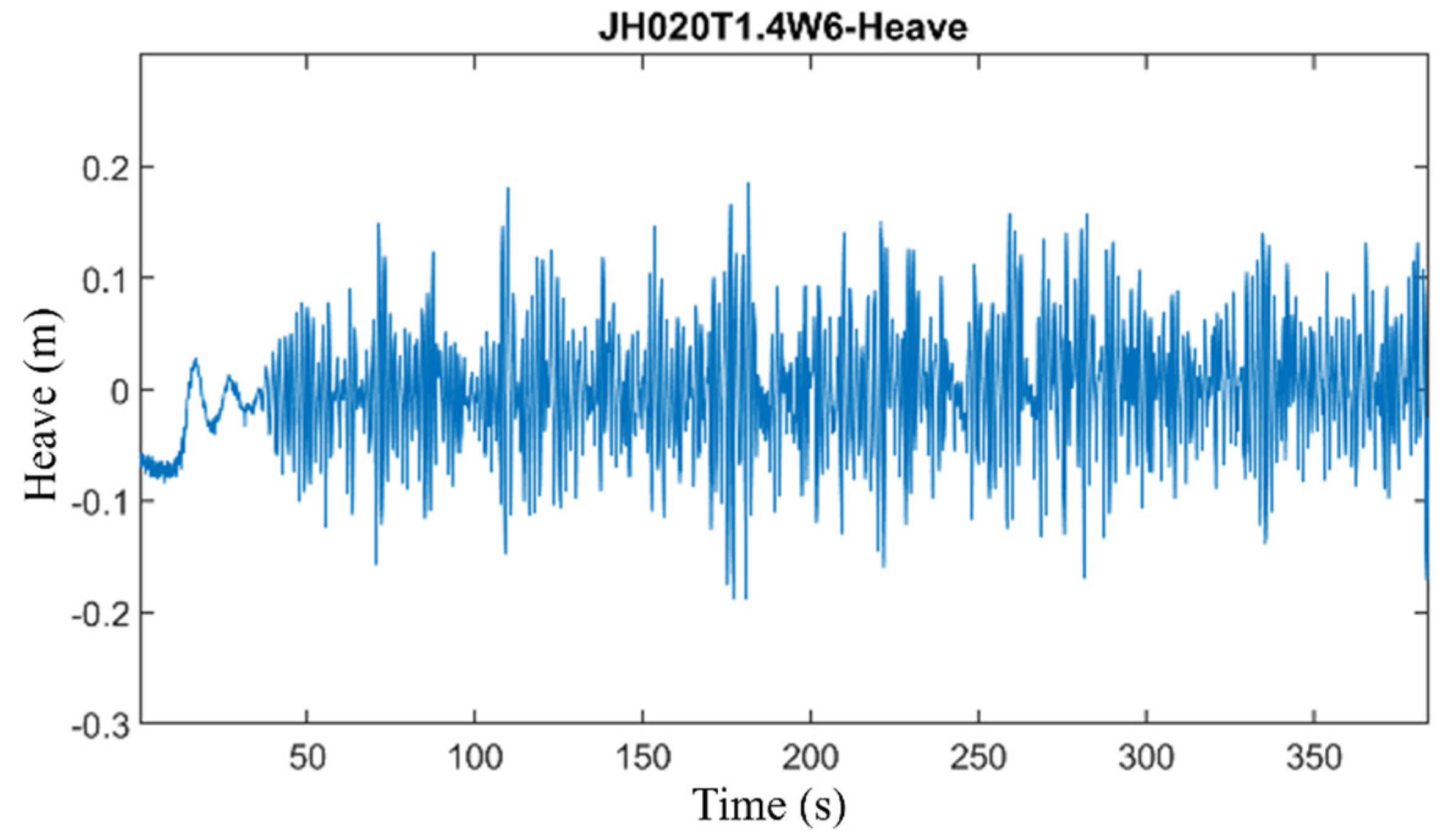
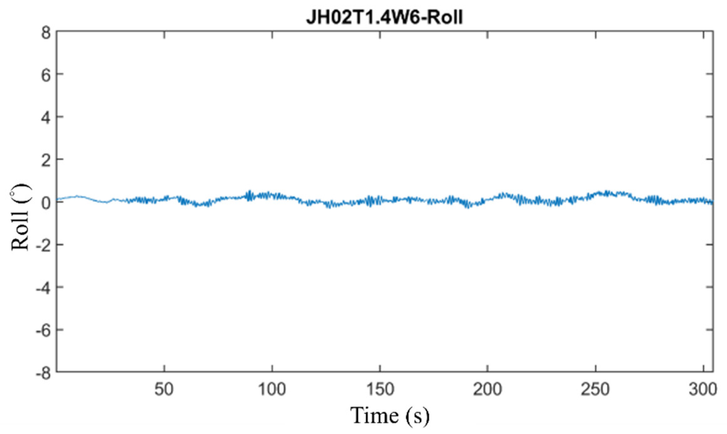
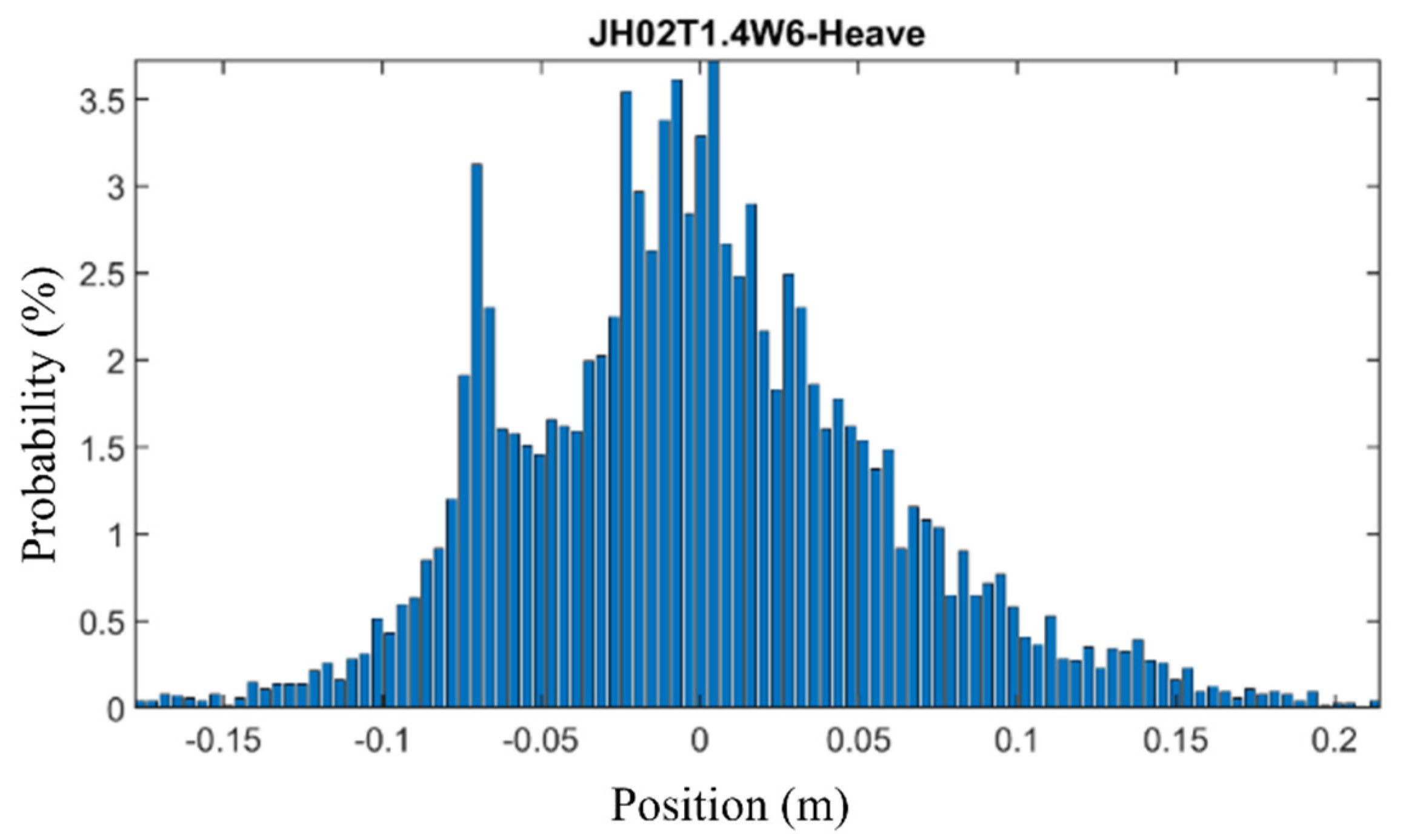
3.6. Motion and Tension Results from Experiment

Figure 37, Figure 38, Figure 39, Figure 40 and Figure 41 show the motion of the floating platform under the combined effect of irregular waves and wind directions in normal sea conditions. In normal sea conditions, the displacement of the floating platform in the surge direction was about 0.5 m, the response amplitude of the floating platform in the heave direction was about ±0.2 m, the pitch angle changed within ±2°. There was no obvious motion response in the roll and yaw.

Figure 42, Figure 43, Figure 44 and Figure 45 show the probability distribution of the floating platform in the surge, heave, and pitch motions under wave and wind directions in normal sea conditions. Regarding the surge motion, it can be seen that the displacement distance of the floating platform was concentrated within the range of 0.28 m–0.35 m. The motion amplitude in the heave motion was concentrated within the range of ±0.05 m, and the pitch motion was in the range of −0.5–0.8°. Figure 42 shows the time series of tension in normal sea conditions. Under wave–wind combined conditions, the average tension was 145 N, and the instantaneous maximum tension was 319 N. For normal sea conditions, wind force had a significant effect on the average tension and instantaneous extreme tension of the mooring line. The reason was that the structure of the FPV system was nearly above the water surface, so the effect of wind thrust was much more dominant than local wind waves. However, the cable tension was still much smaller than the breaking load of the chain of R4, at 58,320 N under normal conditions.

By comparing the AQWA and experiment results, the motion responses of FPV are listed in

Table 6. The motion response comparison between AQWA and experiment.

	Motion Response of FPV
	Surge	Heave	Pitch
AQWA	1.0 m	±0.03 m	±2°
Experiment	0.5 m	±0.2 m	±2°

. The results were almost the same in the pitch motion but much more different in surge and heave motions. The main difference between AQWA and the experiment was in the viscosity factor. It can be observed that the heave motion of FPV was affected by the water in the damping pool, which caused the FPV platform vibration in the experiment. In general, the simulation of FPV in normal sea conditions and extreme sea conditions by AQWA is a more prudent choice for the design of the FPV system.

4. Conclusions

This study focused on the motion characteristic of an FPV platform and the pressure distribution of solar panels under normal sea conditions and extreme sea conditions, respectively. Through the numerical simulation and experimental results, several conclusions are summarized as follows:

• Based on the results of free decay test simulation and fast Fourier transform, it is revealed that the natural period of the FPV platform was within 2 seconds in the heave and pitch directions, which indicates that the floating platform was prone to resonance in high-frequency wave conditions. Hence, careful consideration should be given to the stability of the FPV structure.
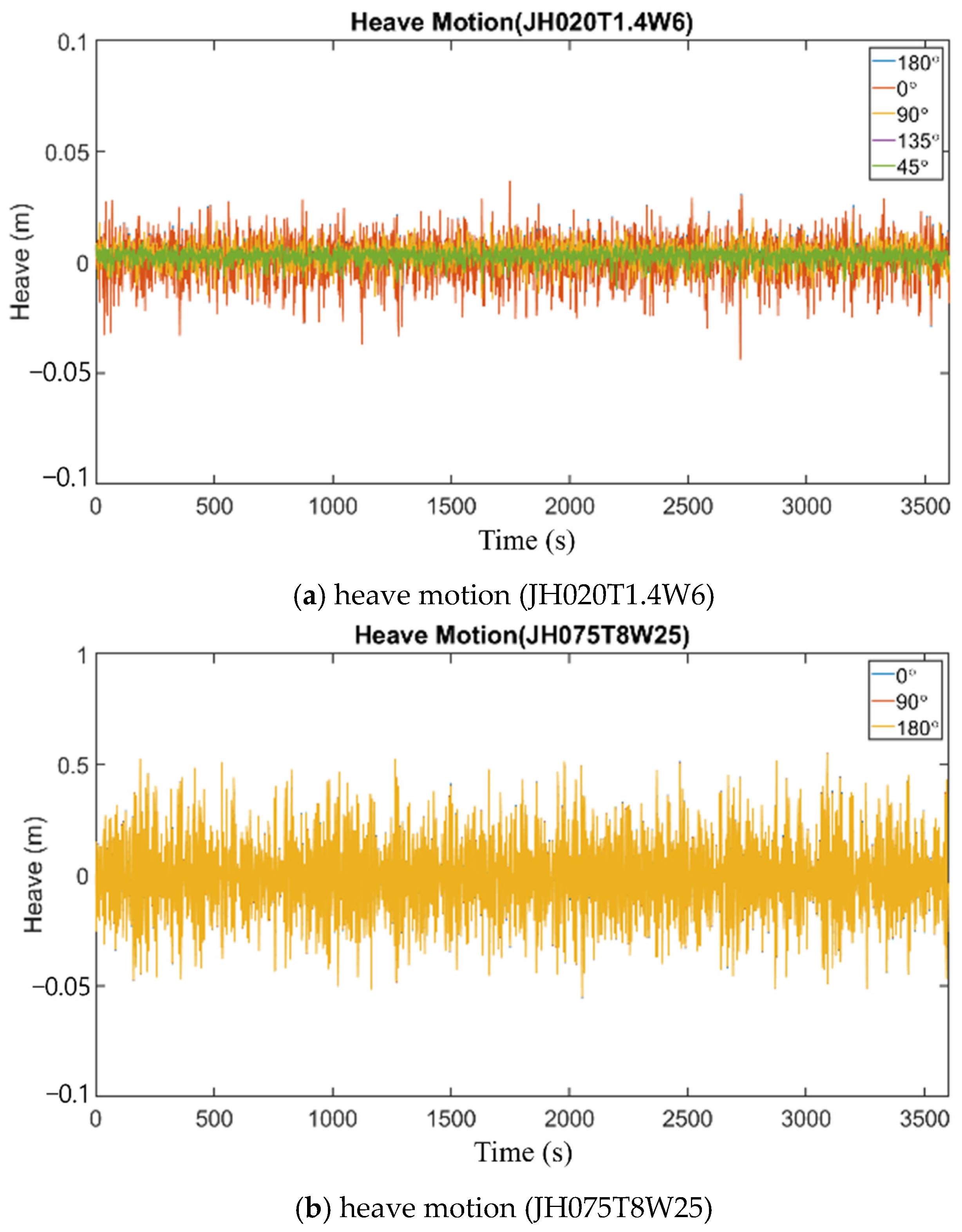
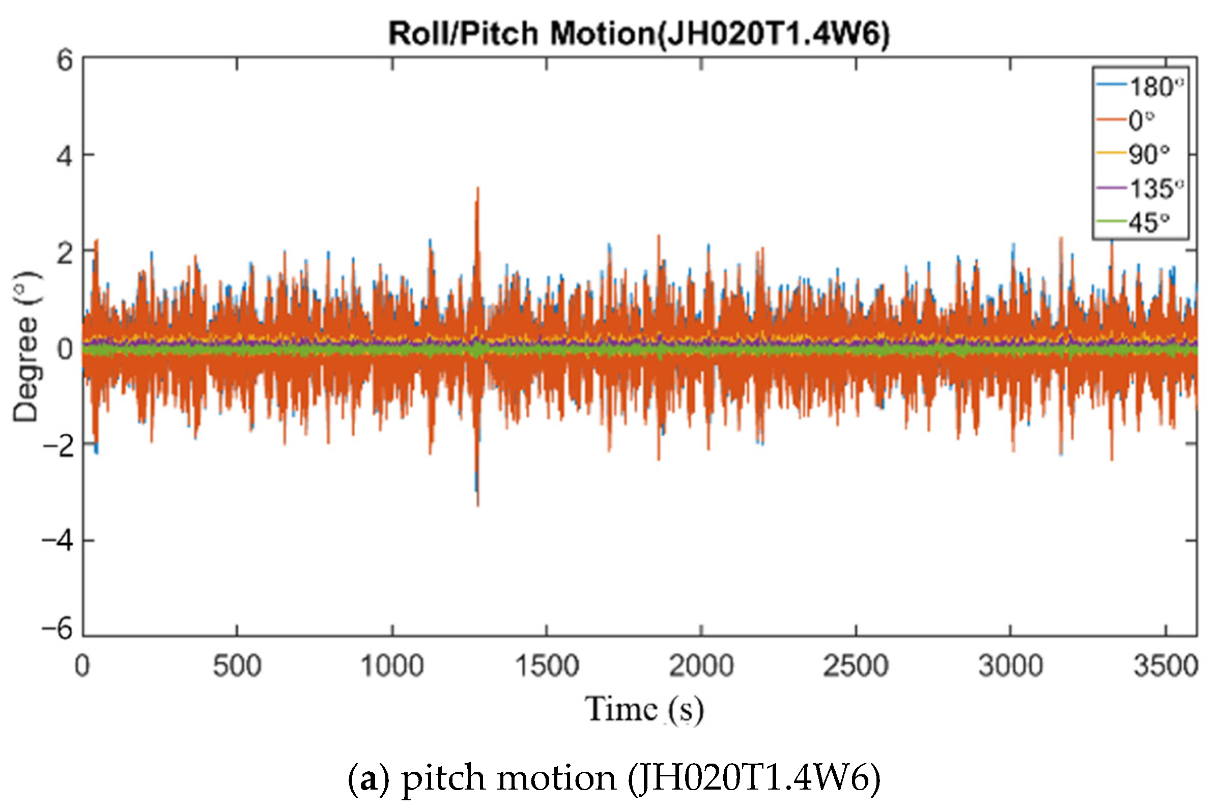
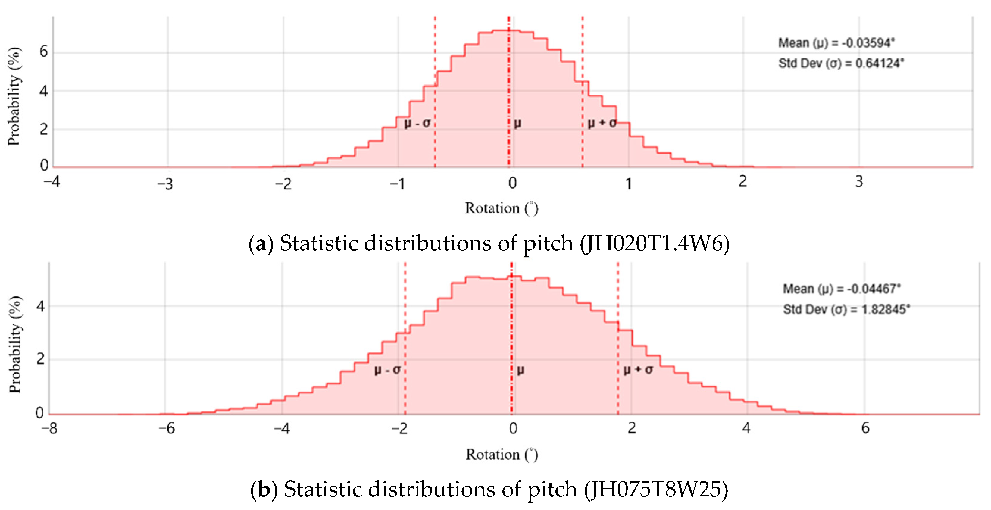
• According to the simulation results of extreme sea conditions in this study, the pitch motion of the floating platform changed about ±6° without overturning; however, the stability of the FPV system should still be monitored in field applications. Meanwhile, under normal sea conditions, the angle of the FPV platform varied within ±2°, which shows that the power generation efficiency can be ensured.
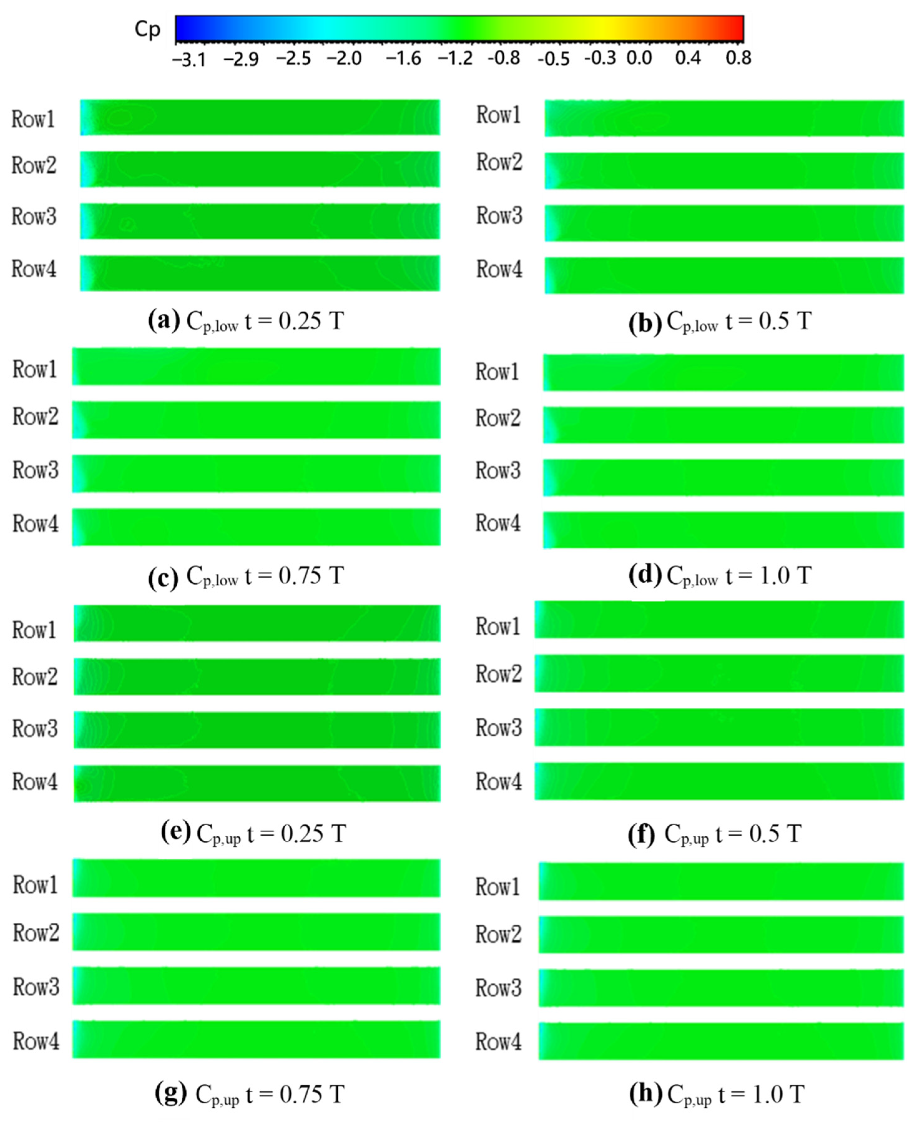
• For the distribution of the surface pressure coefficient of the solar panel, the cases of different wave and wind directions were investigated in this study. It was observed that once the front edge of the solar photovoltaic panel was in contact with the incoming wind, a separated flow would be generated, and then the circulation airflow would be generated upstream of the solar photovoltaic panel to form a negative pressure area. At the two edges of the short sides, angular vortices were formed at the relative positions due to the downward air curling up on the upper surface, indicating that the front edge and side edges of the solar photovoltaic panel were easily affected by the wind flow, thus affecting its stability.
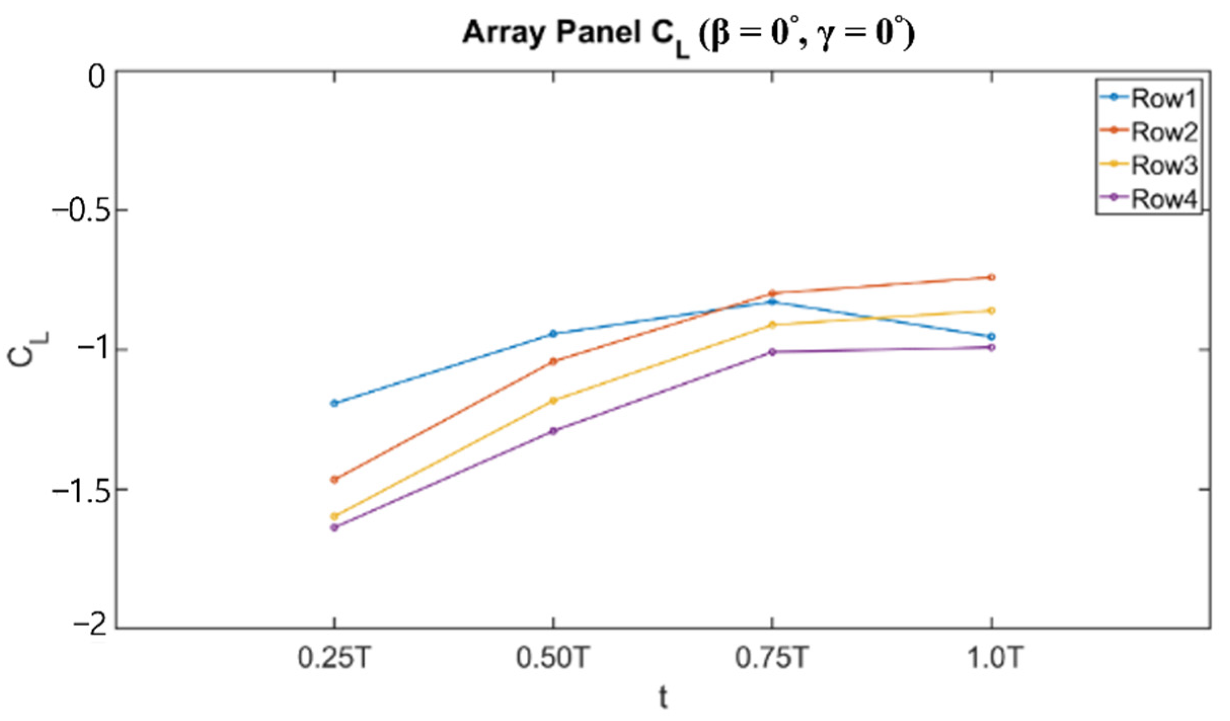
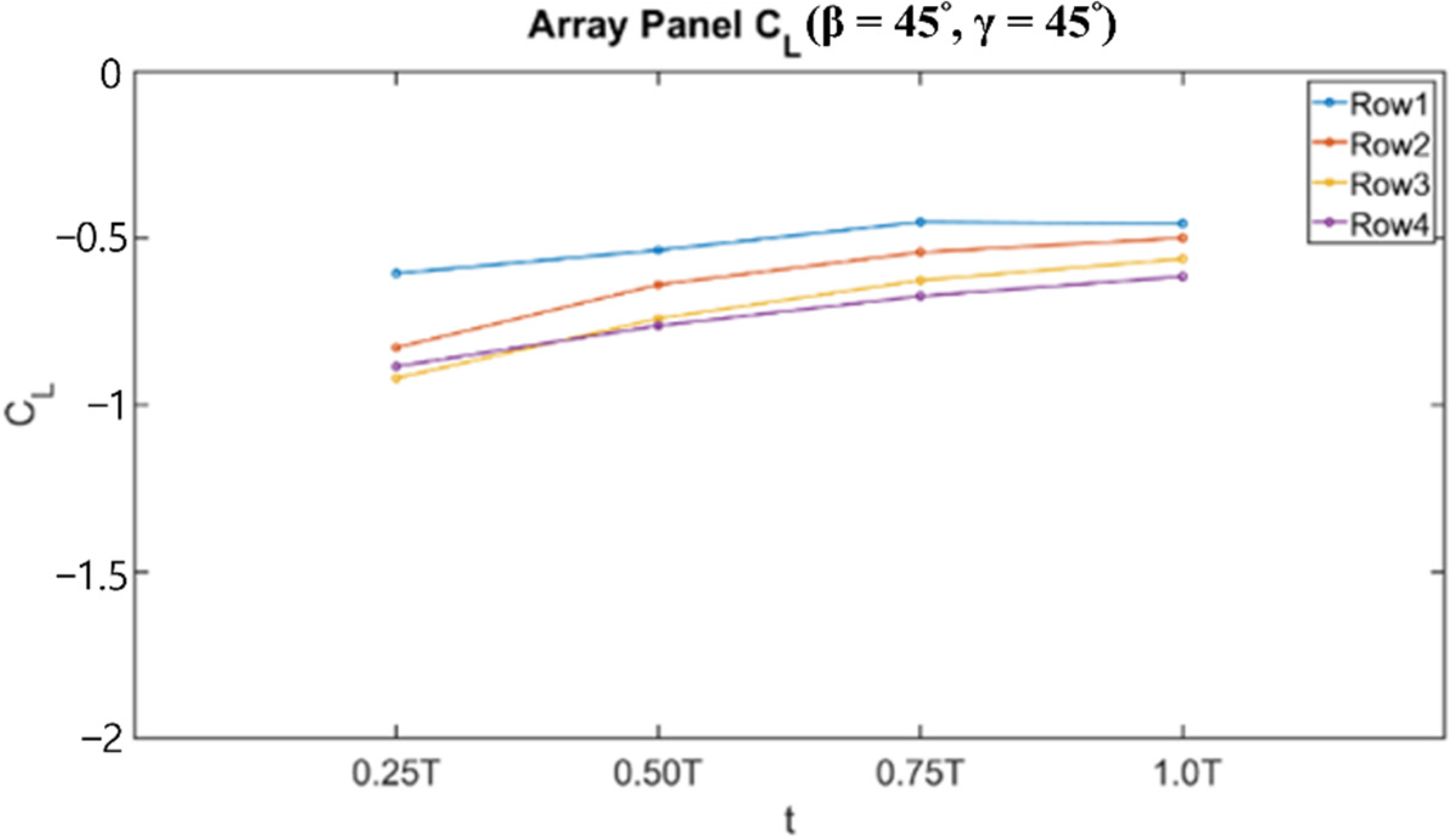
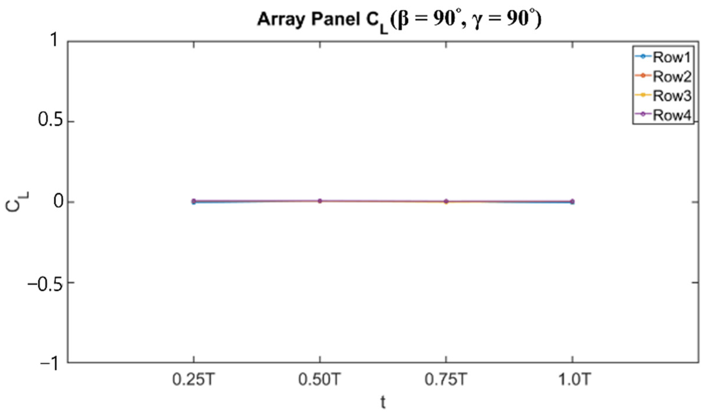
• From the surface pressure coefficient patterns, it can be derived that when the wind direction changed, the upper and lower surface pressure distribution of the solar panels would also shift accordingly. According to the lift coefficient results, it is found that when the wave period stage changed with different angles between wave and wind loads, the lift coefficient increased with the increasing angle between wave and wind loads. However, there was a maximum lift force when the wave and wind directions were 0° and t = 0.25T.

References

1. Sahu, A.; Yadav, N.; Sudhakar, K. Floating photovoltaic power plant: A review. Renew. Sustain. Energy Rev. 2016, 66, 815–824. [Google Scholar] [CrossRef]
2. IRENA. Renewable Capacity Highlights. 2020. Available online: https://www.irena.org/-/media/Files/IRENA/Agency/Publication/2021/Apr/IRENA_-RE_Capacity_Highlights_2021.pdf?la=en&hash=1E133689564BC40C2392E85026F71A0D7A9C0B91 (accessed on 18 September 2020).
3. Rosa-Clot, M.; Tina, G.M. Current Status of FPV and Trends. In Floating PV Plants; Elsevier: Amsterdam, The Netherlands, 2020; pp. 9–18. [Google Scholar]
4. DNV GL. DNVGL-RP-0584. Design Development and Operation of Floating Solar Photovoltaic Systems. 2021. Available online: https://rules.dnv.com/docs/pdf/DNV/RP/2021-03/DNVGL-RP-0584.pdf (accessed on 22 May 2021).
5. World Bank Group. Where Sun Meets Water-Floating Solar Market Report; World Bank Group: Washington, DC, USA, 2018. [Google Scholar]
6. Oliveira-Pinto, S.; Stokkermans, J. Assessment of the potential of different floating solar technologies—Overview and analysis of different case studies. Energy Convers. Manag. 2020, 211, 112747. [Google Scholar] [CrossRef]
7. Trapani, K.; Santafé, M.R. A review of floating photovoltaic installations: 2007–2013. Prog. Photovolt. Res. Appl. 2015, 23, 524–532. [Google Scholar] [CrossRef] [Green Version]
8. Liu, L.; Wang, Q.; Lin, H.; Li, H.; Sun, Q. Power Generation Efficiency and Prospects of Floating Photovoltaic Systems. Energy Procedia 2017, 105, 1136–1142. [Google Scholar] [CrossRef]
9. Cazzaniga, R.; Cicu, M.; Rosa-Clot, M.; Rosa-Clot, P.; Tina, G.M.; Ventura, C. Floating photovoltaic plants: Performance analysis and design solutions. Renew. Sustain. Energy Rev. 2018, 81, 1730–1741. [Google Scholar] [CrossRef]
10. Campana, P.E.; Wästhage, L.; Nookuea, W.; Tan, Y.; Yan, J. Optimization and assessment of floating and floating-tracking PV systems integrated in on- and off-grid hybrid energy systems. Sol. Energy 2019, 177, 782–795. [Google Scholar] [CrossRef]
11. Kim, S.-H.; Yoon, S.J.; Choi, W.; Choi, K.B. Application of Floating Photovoltaic Energy Generation Systems in South Korea. Sustainability 2016, 8, 1333. [Google Scholar] [CrossRef] [Green Version]
12. Jamalludin, M.A.S.; Muhammad-Sukki, F.; Abu-Bakar, S.H.; Ramlee, F.; Munir, A.B.; Bani, N.A.; Muhtazaruddin, M.N.; Mas’ud, A.A.; Ardila-Rey, J.A.; Ayub, A.S.; et al. Potential of floating solar technology in Malaysia. Int. J. Power Electron. Drive Syst. (IJPEDS) 2019, 10, 1638–1644. [Google Scholar] [CrossRef] [Green Version]
13. Silvério, N.M.; Barros, R.M.; Tiago Filho, G.L.; Redón-Santafé, M.; dos Santos, I.F.S.; de Mello Valerio, V.E. Use of floating PV plants for coordinated operation with hydropower plants: Case study of the hydroelectric plants of the São Francisco River basin. Energy Convers. Manag. 2018, 171, 339–349. [Google Scholar] [CrossRef]
14. Rauf, H.; Gull, M.S.; Arshad, N. Integrating Floating Solar PV with Hydroelectric Power Plant: Analysis of Ghazi Barotha Reservoir in Pakistan. Energy Procedia 2019, 158, 816–821. [Google Scholar] [CrossRef]
15. Mittal, D.; Saxena, B.K.; Rao, K.V.S. Floating solar photovoltaic systems: An overview and their Feasibility at kota in Rajasthan. In Proceedings of the International Conference on Circuits Power and Computing Technologies, Kollam, India, 20–21 April 2017. [Google Scholar]
16. Hsu, S.-T.; Lin, W.-Y.; Wu, J.-J. Environmental Factors of non-unitorm Dynamic Mechanical Load Test due to Wind Actions on Photovoltaic Modules. Energy Procedia 2018, 150, 50–57. [Google Scholar] [CrossRef]
17. Choi, Y.-K. A Study on Power Generation Analysis of Floating PV System Considering Environmental Impact. Int. J. Softw. Eng. Its Appl. 2014, 8, 75–84. [Google Scholar] [CrossRef]
18. ANSYS. Aqwa Theory Manual. Available online: https://cyberships.files.wordpress.com/2014/01/wb_aqwa.pdf (accessed on 16 July 2020).
19. ANSYS. ANSYS Fluent Theory Guide. Available online: https://www.afs.enea.it/project/neptunius/docs/fluent/html/th/main_pre.htm (accessed on 22 August 2020).
20. Su, K.-C.; Chung, P.-H.; Yang, R.-Y. Numerical simulation of wind loads on an offshore PV panel. J. Mech. 2020, 37, 53–62. [Google Scholar] [CrossRef]
21. Menter, F.R. Two-equation eddy-viscosity turbulence models for engineering applications. AIAA J. 1994, 32, 1598–1605. [Google Scholar] [CrossRef] [Green Version]
22. SHIH, T.-H.; Liou, W.W.; Shabbir, A.; Yang, Z.; Zhu, J. A new k-e eddy-viscosity model for high Reynolds number turbulent flows. Compurers Fluid 1995, 24, 227–238. [Google Scholar] [CrossRef]
23. Chung, P.-H.; Chou, C.C.; Yang, R.Y.; Chung, C.Y. Wind Loads on a PV Array. Appl. Sci. 2019, 9, 2466. [Google Scholar] [CrossRef] [Green Version]
24. Chuang, T.-C.; Yang, W.-H.; Yang, R.-Y. Experimental and numerical study of a barge-type FOWT platform under wind and wave load. Ocean Eng. 2021, 230, 109015. [Google Scholar] [CrossRef]
25. Chung, K.-M.; Chang, K.-C.; Chou, C.-C. Wind loads on residential and large-scale solar collector models. J. Wind Eng. Ind. Aerodyn. 2011, 99, 59–64. [Google Scholar] [CrossRef]
Figure 1. Photo of solar power station in the intertidal zone, midwestern Taiwan.
Energies 14 07789 g001
Figure 2. Sketch of FPV model.
Energies 14 07789 g002
Figure 3. The mooring system of FPV system ((a) lateral view and (b) top view) used in AQWA.
Energies 14 07789 g003
Figure 4. (a) Computation domain and (b) mesh of FPV system used in FLUENT.
Energies 14 07789 g004
Figure 5. Photo of FPV model scaled by 1:4 scale ratio.
Energies 14 07789 g005
Figure 6. (a) Tension static test comparison of the modified values for the scaled model and (b) photo of mooring line.
Energies 14 07789 g006
Figure 7. (a) Photo and (b) schematic diagram of wave/wind/current basin.
Energies 14 07789 g007
Figure 8. Sensor locations of experimental setup.
Energies 14 07789 g008
Figure 9. Schematic diagram of wave and wind direction under (a) normal sea conditions and (b) extreme sea conditions.
Energies 14 07789 g009
Figure 10. Natural period of the FPV system under (a) heave, (b) roll, and (c) pitch modes.
Energies 14 07789 g010
Figure 11. Motion trajectory in (a) normal sea conditions and (b) extreme sea conditions.
Energies 14 07789 g011aEnergies 14 07789 g011b
Figure 12. Surge motion in (a) normal sea conditions and (b) extreme sea conditions.
Energies 14 07789 g012
Figure 13. Heave motion in (a) normal sea conditions and (b) extreme sea conditions.
Energies 14 07789 g013
Figure 14. Pitch motion in (a) normal sea conditions and (b) extreme sea conditions.
Energies 14 07789 g014aEnergies 14 07789 g014b
Figure 15. Statistical distributions of surge motion of platform in (a) normal sea conditions and (b) extreme sea conditions.
Energies 14 07789 g015
Figure 16. Statistical distributions of heave motion of platform in (a) normal sea conditions and (b) extreme sea conditions.
Energies 14 07789 g016
Figure 17. Statistical distributions of pitch motion of platform in (a) normal sea conditions and (b) extreme sea conditions.
Energies 14 07789 g017
Figure 18. Time series of tension (JH020T1.4W6).
Energies 14 07789 g018
Figure 19. Time series of tension (JH075T8W25).
Energies 14 07789 g019
Figure 20. Per unit period time series of pitch angle motion of (a) normal sea conditions and (b) extreme sea conditions.
Energies 14 07789 g020
Figure 21. Pressure coefficient pattern for β = 0° and γ = 0°: (ad) are lower surface patterns; (eh) are upper surface patterns.
Energies 14 07789 g021
Figure 22. Pressure coefficient pattern for β = 45° and γ = 45°: (ad) are lower surface patterns; (eh) are upper surface patterns.
Energies 14 07789 g022
Figure 23. Pressure coefficient pattern for β = 90° and γ = 90°: (ad) are lower surface patterns; (eh) are upper surface patterns.
Energies 14 07789 g023
Figure 24. Pressure coefficient pattern for β = 135° and γ = 135°: (ad) are lower surface patterns; (eh) are upper surface patterns.
Energies 14 07789 g024
Figure 25. Pressure coefficient pattern for β = 180° and γ = 180°: (ad) are lower surface patterns; (eh) are upper surface patterns.
Energies 14 07789 g025
Figure 26. Pressure coefficient pattern for β = 0° and γ = 0°: (ad) are lower surface patterns; (eh) are upper surface patterns.
Energies 14 07789 g026
Figure 27. Pressure coefficient pattern for β = 90° and γ = 0°: (ad) are lower surface patterns; (eh) are upper surface patterns.
Energies 14 07789 g027
Figure 28. Pressure coefficient pattern for β = 180° and γ = 0°: (ad) are lower surface patterns; (eh) are upper surface patterns.
Energies 14 07789 g028
Figure 29. Lift coefficient for the case of γ = 0° and β = 0°.
Energies 14 07789 g029
Figure 30. Lift coefficient for the case of γ = 45° and β = 45°.
Energies 14 07789 g030
Figure 31. Lift coefficient for the case of γ = 90° and β = 90°.
Energies 14 07789 g031
Figure 32. Lift coefficient for the case of γ = 135° and β = 135°.
Energies 14 07789 g032
Figure 33. Lift coefficient for the case of γ = 180° and β = 180°.
Energies 14 07789 g033
Figure 34. Lift coefficient for the case of γ = 0° and β = 0°.
Energies 14 07789 g034
Figure 35. Lift coefficient for the case of γ = 0° and β = 90°.
Energies 14 07789 g035
Figure 36. Lift coefficient for the case of γ = 0° and β = 180°.
Energies 14 07789 g036
Figure 37. Experimental result of surge motion in normal sea conditions.
Energies 14 07789 g037
Figure 38. Experimental result of heave motion in normal sea conditions.
Energies 14 07789 g038
Figure 39. Experimental result of roll motion in normal sea conditions.
Energies 14 07789 g039
Figure 40. Experimental result of pitch motion in normal sea conditions.
Energies 14 07789 g040
Figure 41. Experimental result of yaw motion in normal sea conditions.
Energies 14 07789 g041
Figure 42. Experimental result of probability distribution in the surge motion.
Energies 14 07789 g042
Figure 43. Experimental result of probability distribution in the heave motion.
Energies 14 07789 g043
Figure 44. Experimental result of probability distribution in the pitch motion.
Energies 14 07789 g044
Figure 45. Experimental result of time series of tension in normal sea conditions.
Energies 14 07789 g045