Abstract
This paper looks at a typical problem encountered in the process of designing an automatic ship’s course stabilisation system with the use of a relatively new methodology referred to as the Active Disturbance Rejection Control (ADRC). The main advantage of this approach over classic autopilots based on PID algorithms, still in the majority, is that it eliminates the tuning problem and, thus, ensures a much better average performance of the ship in various speed, loading, nautical and weather conditions during a voyage. All of these factors call for different and often dynamically variable autopilot parameters, which are difficult to assess, especially by the ship’s crew or owner. The original result of this article is that the required controller parameters are approximated based on some canonical model structure and analysis of the hydrodynamic properties of a wide class of ships. Another novelty is the use of a fully verified, realistic numerical hydrodynamic model of the ship as a simulation model as well as a basis for deriving a simplified model structure suitable for controller design. The preliminary results obtained indicate good performance of the proposed ADRC autopilot and provide prospects for its successful implementation on a real ship.
1. Introduction
A good design of a ship and her steering control system is crucial for the safety and efficiency, or fuel economy, of the operation (navigation) process. Sometimes, and to some extent, a good control system can even enhance the actual poor design of the ship’s hull, propeller and rudder, especially in heavy weather conditions.
Ship steering, realized either by automatic (autopilot) or manual (human) control, is twofold. First, it consists of course-keeping that is following a predetermined heading (most frequent) or track (as in modern integrated navigation systems). Second, it includes course-changing manoeuvres to reach the next straight-line section (leg) of the route according to the voyage plan or as a part of collision avoidance. In both of these tasks, the steering optimization by the proper selection of an autopilot structure/design and the tuning of its parameters can render better energy efficiency. For example, the problem with the often inappropriate tuning of the classic PID (Proportional–Integral–Derivative) regulators is the cause of significant energy (fuel) losses resulting from excessive ship’s yawing as well as excessive wear of the steering gear. Generally a properly tuned autopilot throughout the whole ship’s voyage is a crucial factor in the energy saving issue [1].
Real-life conditions are characterized by various types of uncertainties, such as inaccuracies in the system model, the occurrence of random processes such as winds, waves or currents, and other exogenous effects. Therefore, when designing the ship’s control system, it is necessary to use techniques that take into account the nonlinear effects of the process and the parametric uncertainty of the ship’s model [2].
There are many works on ship autopilots. Apart from the classic PIDs, there are more and more works on autopilots based on modern control algorithms, e.g., nonlinear [2] robust, adaptive [3,4] or intelligent [5]. Among those that deserve attention, there are also autopilots based on the ADRC algorithm [6].
However, their simulation verification (except classical sea trials) has usually been performed on simplified and not fully validated models [6]. Moreover, they often require the tuning of a number of parameters [7,8] (which often is only possible offline using AI-type algorithms) or some detailed knowledge about the ship, obtained, for example, from sea trials or identification procedures [9].
A comparative analysis of control performance obtained via the ADRC versus a traditional autopilot based on the PID algorithm is discussed in [10]. However, the data (ship model parameters) used there relate to the training ship Blue Lady, a physical model of the tanker made in 1:24 scale [11,12]. Therefore, the results obtained in the present research are practically more representative.
The problems of ship steering control design are wide and complex [13]. We can often define them in terms of classical optimisation, specifying an objective function as spread on the controller’s model structure and parameters and minimising/maximising it to obtain the ‘optimal’ design. Such an optimality appears, however, to be mostly local, for very specific conditions of the ship and environment, and the control often fails as it is very sensitive to model uncertainty and disturbances, as with PID controllers and other controllers designed using so-called optimal control techniques [13,14,15]. This is why other approaches are being sought, e.g., a disturbance observer-based control (DOBC) [13,16] and the relatively new ADRC method being investigated in the present work. According to its specific type, the rather fixed structure of an ADRC controller (additionally of partly non-parametric definition) cannot easily undergo an optimisation in a mathematical sense.
The stipulated energy efficiency for an ADRC controller, for all ship operational conditions, is treated hereafter qualitatively rather than quantitatively. This is also partly due to this being the preliminary stage of our ADRC development in the ship steering domain, and there being limited performance test results. At this moment, the ADRC is expected to be at least equivalent to the PID controller but without its ‘local’ features, and, hence, (as presenting with no need of tuning) can be deemed more effective over the whole ship’s operational lifetime or mission profile. For industrial implementation, as the next step to our commonly accepted MATLAB/Simulink-based studies in this paper, a more comprehensive and quantitative comparison of various controllers, and for various ships, is being scheduled in the future. This would involve different energy-efficiency indicators and hardware-in-the-loop (HIL) studies, especially on the full-mission ship-handling simulator at the authors’ premises (Maritime University of Szczecin, Poland), and full-scale trials.
The Active Disturbance Rejection Control (ADRC) method, originally proposed by Han in 1989 [17,18], is an innovative approach to the control of a plant whose dynamic properties are uncertain and affected by external disturbances. Han’s concept is based on the use of an extended state observer in the control loop (ESO).
The observer, apart from tracking the values of state variables, supports the estimation of a certain virtual variable consisting of combined external disturbances and components resulting from the uncertainty of the plant parameters and its nonlinearities.
The ADRC methodology has been gaining in popularity [19,20]. It should be noted here that, although based on the concept of ESO, it incorporates other ingredients, such as the transient profile generator, noise-tolerant tracking differentiator or special nonlinear feedback [17]. Regardless, it seems that the estimation of total disturbance and rejection of the same, discussed in this paper, are of key importance here.
Considering that complex control systems can be typically reduced to the first or second order, the ADRC facilitates the procedure through a joint treatment of external disturbances and uncertainty modelling. Since little knowledge is required of the process and the disturbance model, the ADRC can exercise effective control over a complex system in the absence of a detailed and accurate mathematical model. Owing to its simplicity, the technique is an attractive alternative to much more advanced model-based approaches, such as designs based on adaptive and/or robust control methodologies [4]. Thereby, practitioners looking for more efficient algorithms than the standard PID can consider using the ADRC.
The paper comprises six sections concluded with a discussion. In Section 2, the principal concept of the ADRC control design is explained, followed with a description of the mathematical model of the ship’s dynamics in Section 3. In Section 4, zero dynamics and a model suitable for the controller design are discussed. In Section 5, the authors explain how to design an autopilot using the ADRC technique. The final Section 6 and Section 7 include simulation tests and their results, followed with a discussion.
2. The Principal Concept of the ADRC Control
Let us explain the main idea behind the ADRC control technique. Rather than formal proof, we focus on an intuitive analysis of the system output stabilization. For simplicity and clarity, yet without losing generality, the following second order, SISO, nonlinear affine system should be considered
where
—state variables,
u—control variable,
y—system output,
f and c—known function and constant respectively,
d—known disturbance.
It should be borne in mind that these considerations apply as well to a general nonlinear model in the canonical (Brunovsky) form.
In order to stabilize the system output at the assumed set-point , a simple feedback linearizing controller can be applied
where represents the desired output, while and are the controller gains.
To make the calculation more realistic, let us assume that the function f is unknown and the parameter c is uncertain, i.e.,: , where is its known estimate (cf. Section 3, Section 4 and Section 5), while represents its range of uncertainty. Additionally, the system is exposed to the unknown exogenous load disturbances d(t).
On the basis of the above, the following is obtained
For the purpose of designing a stabilizing controller, all system uncertainties shall be grouped into a single expression , which represents generalized or total disturbances.
In the next step, a subsequent state variable is introduced. Assuming that where G(t) is unknown, we obtain a formally equivalent and always observable system
If all the state vector components are available, the controller of the linear system above (4) (including the ‘virtual’ disturbance G(t)), can be expressed with the following formula (cf. (2))
Note that with the controller expressed with (5), the disturbance is cancelled, and the remainder is a PD-type algorithm. This way, our system, written in the form (4), (5) has a completely known form
Hence, its behaviour can be determined precisely via proper selection of the controller gains (e.g., by the pole-placement or LQR technique [21]) under laboratory conditions. Thus, in the further part we assume that and are known (cf. (38)). The key now is to have all the state vector components available.
The next and last step of the ADRC methodology is the design of an observer [21]. For this purpose, (4) is expressed in the matrix form. The observer is, obviously, designed for a disturbance-free system, i.e., a system expressed as follows
In the formalism above, F(t) is perceived by the state observer as a constant state variable (cf. the third equation, where ). Hence, the reconstruction of exact state can take place only in the steady-state , .
There is a permanent transient process for non-constant disturbances (such as in the event of a step change of the set-point ), where the observer state component follows up the varying total disturbance . Implementation of the controller (5) will obviously require a replacement of the original unmeasurable states with their estimates (i = 2,3) using the principle of certainty equivalence.
To summarise the concept of the ADRC controller, let us first write down the general formula for the observer in Kalman form
where L is the observer gain matrix (cf. Section 5).
Now we can obtain its Laplace transform form (for scalar inputs)
where the matrix transfer function is
and I denotes 3 × 3 identity matrix.
Finally, by using (5) we can write the formula for the whole ADRC controller
where the state estimates are taken from (7b).
A natural attempt to formally compare ADRC to a PID controller encounters certain difficulties and methodological challenges. There are some similarities, e.g., ADRC contains PD gains. On the other hand, ADRC does not require direct integral action (which is a weakness of PID). Moreover (as shown in the article), ADRC tuning is global rather than local and, thus, seriously simplified.
3. Ship Manoeuvring Dynamics
3.1. Nonlinear Model
The ship’s motion in the horizontal plane is represented by two vectors of state variables: the position vector [x0, y0, ψ]T, where (x0, y0) and ψ denote earth-based linear position coordinates and angular position (heading), accordingly, and the velocity vector in the ship’s body axes ν = [u, v, r]T, where (u, v) and r are linear velocity components (longitudinal and lateral, or surge and sway) and angular velocity (rate of turn or yaw). The origin is taken at the intersection of the midship section and centreplane, with the ship’s centre of gravity coinciding with this point (usually, at max., a few % of the ship’s length for merchant ships, and of negligible effect in practical manoeuvring). The mentioned former vector is related to the latter one by the kinematic law, whereas the latter is governed by the Newtonian laws of dynamics for a rigid body in fluid (where we adopt Fossen [22] notation)
where M—mass/inertia matrix (including added masses), C—centripetal matrix (also including added masses), D—damping matrix (velocity-related hydrodynamic hull forces), τ—control (external force) vector
In matrix D, we use the following specific expansion of second order (standard form within our research centre)
For our purposes, the component τX in (13) is related only to the propulsive force of the propeller, proportional roughly to its revolutions squared, τX = (1 − tP)·Xnn·n2, where tP—thrust deduction, while the other two components represent the rudder lateral force and moment, τY = Yuuδ·u2δ and τN = Nuuδ·u2δ, respectively (δ < 0 for starboard rudder, in (rad)).
For the purpose of the present research we have adapted the nonlinear model of the slightly unstable large tanker Esso Bernicia, Table 1, that is well published [23] and validated in full scale against widely available and very extensive sea trials. An unstable ship is more challenging for the design and assessment of the autopilot. The selected ship is one of few considered as benchmarks in the area of ship manoeuvring and steering simulation. The original publication [23], however, does not show the exact equations for the structure of forces comprising the listed hydrodynamic derivatives, directly referring to [24]. However, the latter source is too general and has caused a lot of interpretation confusions and, thus, application or implementation problems. A better documentation of the model can be found in [22] that reproduces the original simulation results of [23], but only after correcting the power of the derivatives in the rudder flow speed (‘c’) (also erroneous in [24]) from two to one, which should now look even more natural.

Table 1.
Ship data (ESSO 193 kDWT tanker).
After ensuring that the full model of [22,23] is properly working, and limiting it to the deep water condition, of primary interest in the present preliminary study, we attempted the model simplification to reach the above stated structure with a proper level of adequacy. Our simple standard structure allows to better understand and control the manoeuvring model, as well as to assess the steering simulation results. Among others, the side effect of the propeller, leading to asymmetry in the port and starboard turning circle, was omitted (also of rather negligible effect in the turning circle and zig-zag tests according to the original parameters). In the surge equation, the rudder force and hull resistance coupling with sway velocity also had to be rejected. The other actions are commented on in the annotations (see the footer) to Table 2, which also gathers all of the parameters of our simplified nonlinear model. Instead of a total of 41 derivatives [23], we arrived at 14 derivatives.
Table 2.
Model parameters and hydrodynamic derivatives (full scale, deep water case).
The ‘bis’ superscript, originally used in the symbols of derivatives in [23], is omitted in our presentation, but the necessary scaling/multiplication per the last column of Table 2 should be exercised. The damping derivatives in (14), if not listed in Table 2, equal zero.
We use the unity mass, that means ‘1′ has to be substituted for m in (10) and (11). Since the inertia moment and hydrodynamic forces have already been non-dimensionalised (divided), among others, by the ship’s displacement (mass), providing the derivatives of [23], we can operate our algorithm (by default, assigned to the absolute quantities) almost directly with the non-dimensional parameters. In this case, speaking in general, there is no need to divide force by mass in order to obtain acceleration (for change of velocity) because the non-dimensional forces (and moments), and their components, as combined with the ship’s velocities and some linear dimensions, already represent appropriate linear accelerations (and angular accelerations).
Selected standard manoeuvres of our ship model, to prove its performance, are presented in Appendix A.
3.2. Rudder Dynamics
Ignored in the controller design process, the steering gear model will be part of the overall ship model to ensure that the best possible representation of the real ship dynamics is obtained in the simulations (according to [22])
where ; ; .
3.3. Linearised Model
Assuming that velocity u is not changing considerably during rudder manoeuvres, that is valid, to say, for mild manoeuvres, i.e., with low to medium rudder angles (depending upon inherent nonlinearities in the dynamics of a particular ship) we can linearise the dynamics. Within this condition, the low rudder angles should also be followed by small hull drift angles and dimensionless yaw velocities (corresponding to track curvatures), which are the main factors in hull hydrodynamic forces.
Under the above restraints, (u ≈ const, du/dt = 0), the longitudinal ship dynamic equation now disappears. The other two equations in sway and yaw can be classically and straightforwardly written, with pure derivatives of v and r kept on the left-hand side (and the right-hand side components thus divided by relevant mass-related items), as a set of coupled linear equations of first order (or second order vs. heading ψ, where r = dψ/dt) as follows
where
In the above, with regard to the full equations of sway and yaw of the previous Section 3.1, just two items have been withdrawn, namely and , as producing null partial derivatives versus v and r around the point (u ≠ 0, v = r = 0). One should be aware that all the parameters (mass-related and hydrodynamic derivatives) in Equations (17) and (18) assume the pure numerical values per the second column of Table 2. The mentioned scaling (multiplication by proper power of L) is not required as this has already been incorporated in (17) and (18).
It is remarkable that the reduced, linear ship model (16)–(18) is still unstable on course, although the linearisation (dependent upon a method) often ‘stabilises’ the ship, especially if we identify the linear model from the zig-zag test.
3.4. Rough Estimate of Rudder Moment Derivative b2 for Arbitrary Ship
Since when designing the autopilot algorithm we need at least a rough estimate of the parameter b2 in Equation (16) (see also Section 5 and Section 6)), in this section we derive an approximate formula for b2, valid for a wide class of merchant ships.
The yaw equation taken from (9), while limiting to the rudder moment (denoted by τN) only, i.e., after disregarding matrices C and D, reads
and represents the (additive) contribution of the rudder to the total yaw response. As such, this equation itself also fully describes the ship’s initial motion from rest when hull hydrodynamic forces are not yet developed.
Having adopted the usual, well-known (in ship hydrodynamics) structure of all terms in (19), one obtains the ship’s inertia moment , added inertia and rudder moment , accordingly, as follows
where: m—displacement (mass); —water density; —dimensionless radius of gyration; —dimensionless coefficient of added inertia; —rudder effective abscissa (herein geometrically assumed, = −L/2); —dimensionless hull-rudder interaction coefficient (augmentation of effective rudder lateral force due to hull presence); and —rudder area and its dimensionless coefficient (as ratio of LT), respectively; —rudder flow velocity, i.e., reference velocity in the complicated flow in behind propeller/hull conditions for defining the rudder (dimensionless) force coefficients; —rudder lateral force coefficient, herein equal to the lift coefficient , due to the assumption of the ship’s centreplane straight-line movement).
In the latter, no rudder local drift exists and the rudder angle of attack (‘α’) means rudder angle δ.
Furthermore, we can write down
where: u—ship’s longitudinal speed (as input); displacement (mass); w—wake fraction (dimensionless); —propeller thrust loading coefficient, as based on standard propeller thrust coefficient (‘kT’) and advance ratio (‘J’) and which is constant for the steady-state motion with different propeller rpm.
Herein, the propeller jet velocity is assumed for the reference velocity. However, due to the availability of data and roughness of the approach, we take the free-stream (uniform flow) hydrodynamic characteristics of the rudder in terms of the cL data. This corresponds to null . Note that for other, non-zero values of , the ordinates of cL are always lower.
A straightforward transformation of all the Equations (19)–(27) produces the following simple formula
with
In (29), some items (especially those of hydrodynamic nature) may not be known accurately at the lowest effort. Therefore, the authors recommend using the following data of Table 3 for any ship type (among seagoing merchant ships) and size. These values, together with three geometrical parameters of our tanker in Table 1, namely cB, L and B, return b2 for the speed u = 8.23 m/s equal to −9.18 × 10⁻⁴, as compared to −7.54 × 10⁻⁴ that can be obtained exactly from the parameters of the above ship nonlinear model by means of (16) and (18).
Table 3.
Recommended (rough) values of dimensionless parameters in b2 formula.
For additional guidance and assessment of Table 3, particularly while modelling a class of ships or examining the limits of b2, the reader may refer to the wider literature, for example to:
- Reference [25] for , where even higher values are permitted. Such a significance of has also been proved in the authors’ experience gained through various identification attempts of mathematical ship models. The empirical meaning of this parameter also tends to correct the theoretically assumed , see below, since they both stand beside each other in (23) as a product, taking into account (27);
- Reference [26] for . However, according to the authors’ database, the provided magnitude 0.02 can be somewhat considered as the upper limit for many 1-screw seagoing merchant ships (e.g., tankers, bulk carriers and containerships), where the value 0.015 can often be found in existing ships;
- Reference [27] for . The listed value 2.3 comes from the upper boundary of cL (=1.2), which for the usual rudder aspect (height-to-chord length) ratio of ca. 1.5–1.6 occurs at rudder angle 30° [27];
- Reference [28] for , which reports a range of values 0.05 to 0.062 for . However, this can be easily determined from the actual ship’s longitudinal weight distribution. With such a method, the authors confirmed the data of [28] to be partly correct. Additionally, note that the potential error in the gyration radius is often repaired by the empirical assumption (or full-scale identification) of . The latter is hardly determinable for typical ship hulls, although there are a lot of exact solutions for simple bodies or various regression expressions. In the deep water condition, both the ship’s moment of inertia () and her added inertia () roughly seem to be of the same order and, hence, in Table 3.
The wake fraction and the propeller hydrodynamic characteristics, as well as the propeller selection methods (in terms of rpm, pitch, diameter), are well established in the literature. The practical range of w is approximately 0.3 to 0.45 and depends on whether a ship is slender (e.g., container carrier) or full (e.g., tanker, bulk carrier). Although being partly independent, the propeller thrust loading coefficient cTh varies accordingly between about 1.5 and 3.
4. Zero Dynamics and the Final Controller Design Model
Complex control systems can be typically reduced to the first or second order. Since the ADRC’s order is selected taking into consideration the relative degree [29] of the plant, lumping many non-trackable terms under total disturbance facilitates the simplification.
Applying the input–output (I/O) linearization method, the model is transformed (cf. (16)) as follows
with the output
The resultant form is suitable for direct application of the ADRC technique in accordance with the theory outlined in Section 2. However, in order to avoid the here typical formalism of Lie derivatives, the output (31) is differentiated twice with respect to time, to obtain the equations
where , .
The partial transformation of the coordinates from x to y is defined by the equations
The transformation generates a new system (32) of the second order, representing the external dynamics. Since the original system (30), (31) is of the third order, the missing part of the dynamics must be complemented with the internal (zero) dynamics (of the first order).
An analysis of the system zero dynamics can be performed through examination of the original system (30), (31) under the assumption that its output equals zero . Thereby, we obtain the restricted motion of the system [29], confined to the set
where
The motion of the original system (30), (31) on , with the input (compare (33)), represents the asymptotically stable zero dynamics
Thus, for the purpose of the controller design, the model (30), (31) can be represented by means of the system of second order (32), written as in (1)
5. Autopilot Design Using the ADRC Technique
The ship course-keeping controller will be designed using the ADRC technique discussed above. The ADRC concept is based on the assumption that the object model structure as well as its parameters are unavailable, i.e., the parameters and exogenous disturbances that affect the process are not known. The only known data are the roughly estimated rudder efficiency coefficient of (37) (see (29)). Based on the framework provided by the second-order model (vs. heading) of (37), we can simply apply the theory given in Section 2, in particular Formula (5), defining the controller, and (7) specifying the model for observer design. To maintain consistency with Section 2, denotation of the rudder efficiency coefficient has been changed to . The ADRC controller gains, , have been calculated by the pole-placement method (see (6), (38)), and the observer gain matrix has been tuned using the standard LQR procedure.
6. Simulation Results
Based on the mathematical model of the ship (with the steering gear attached) presented in the previous Sections and the general idea of the ADRC system, simulation tests were carried out using the MATLAB/Simulink environment.
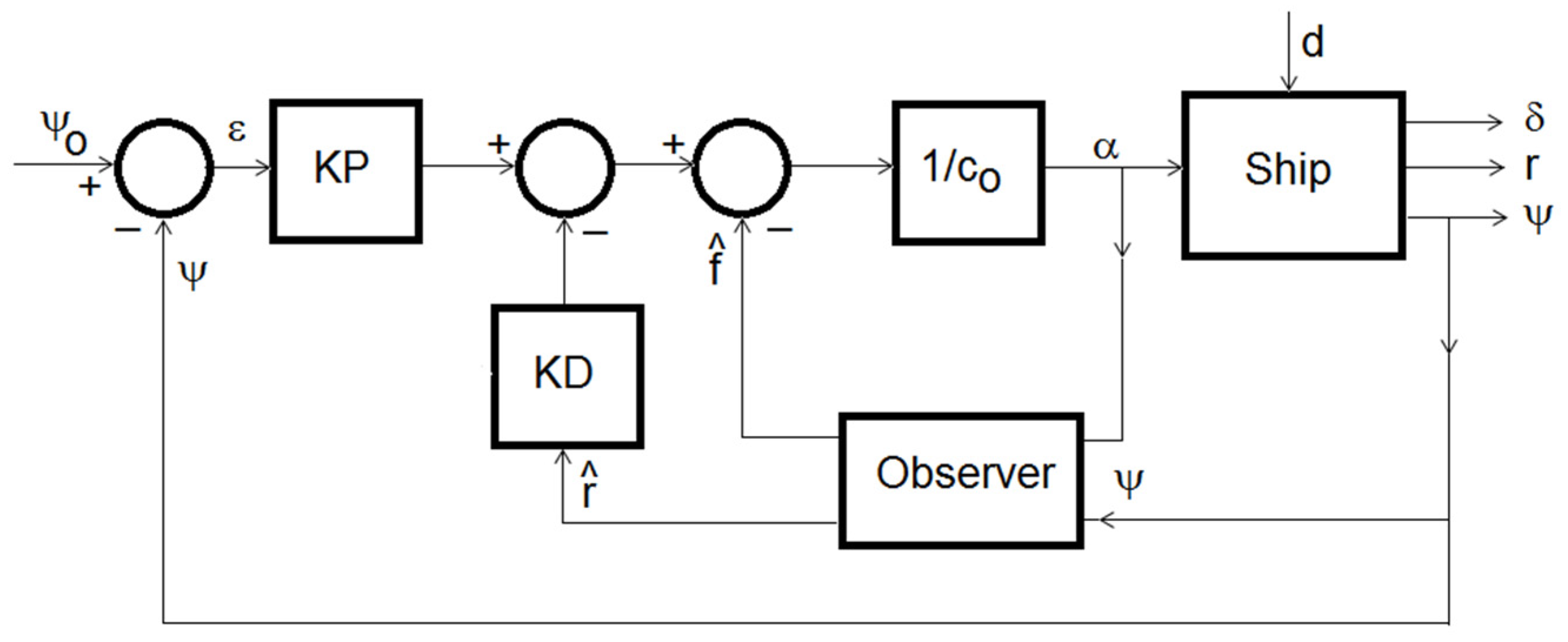
The block diagram of the ADRC-based heading angle control system is shown in Figure 1.
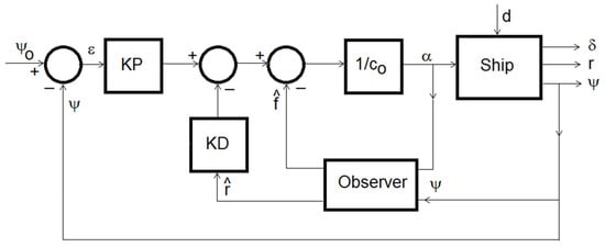
Figure 1.
Block diagram of ADRC heading angle control system.
The following symbols are used: ψ—heading angle, ε—error signal, α—steering gear command, δ—rudder deflection angle, r—angular speed and d—disturbances.
At the first step, it is necessary to determine the parameters of the ADRC system, i.e., , and .
The approximate value of is obtained from the theoretical study (see Section 3.4) where −9.18 × 10⁻⁴ (1/s2). and values are determined via the pole-placement method [30] based on the canonical system (6) as follows
where Tsettle denotes, to some extent, an arbitrarily assumed settling time of the control system (6).
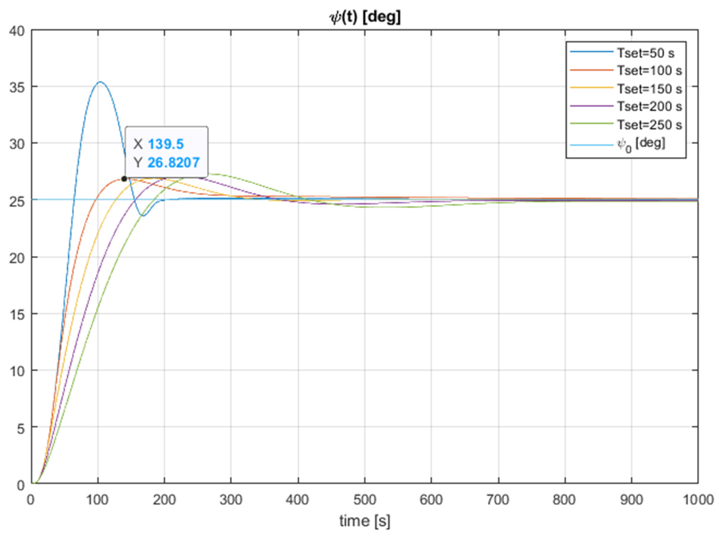
The second step consists of checking the static and dynamic properties of the ADRC system with parameters calculated as above. The results of this experiment are shown in Figure 2.
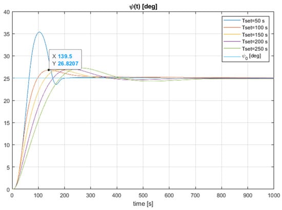
Figure 2.
Static and dynamic behaviour of the ADRC system for different settling time parameter.
In the third stage of the research the robustness of the ADRC system to disturbances was examined.
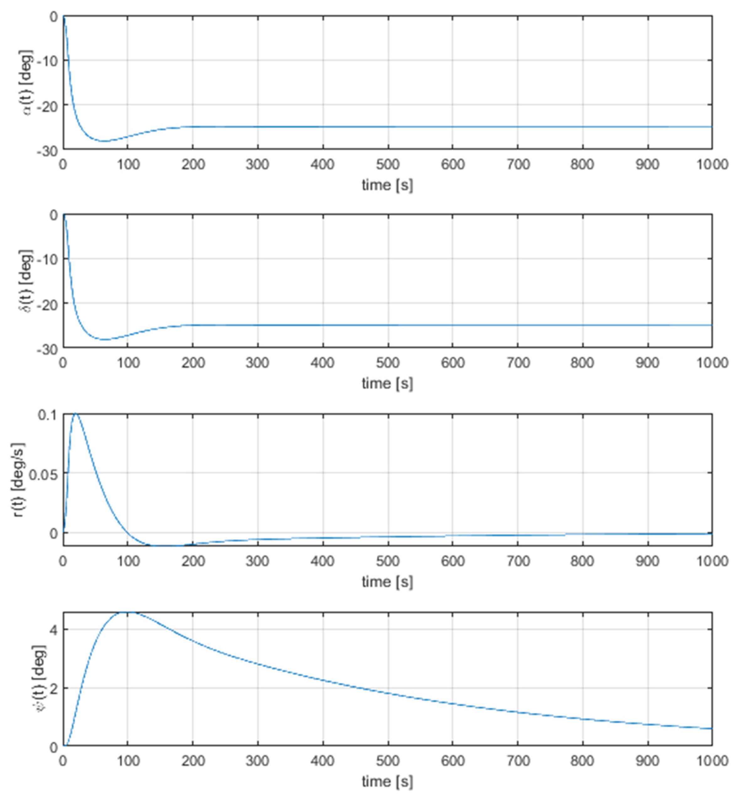
Two kinds of disturbances were selected during the test: constant disturbance of 25 degrees (in terms of the counteracting rudder deflection), which represents the impact of the wind or sea current, and a colourised white noise corresponding to the impact of waves. Results of the simulation with constant disturbance are shown in Figure 3.
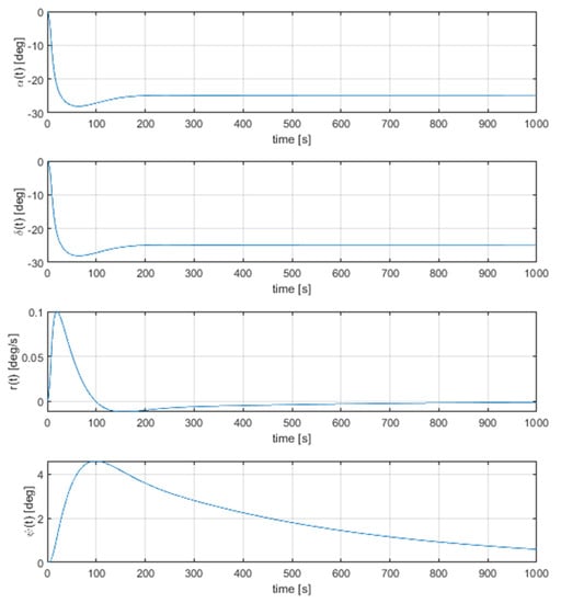
Figure 3.
Reaction of heading angle on constant disturbance.
The noteworthy fact is that the maximal heading angle deviation is about 5 degrees. The steady-state value of the heading angle (not entirely shown in this graph) is equal to zero.
The obtained settling time is calculated for the case when the deviation of the course angle is equal to or less than one degree and amounts to about 800 s.
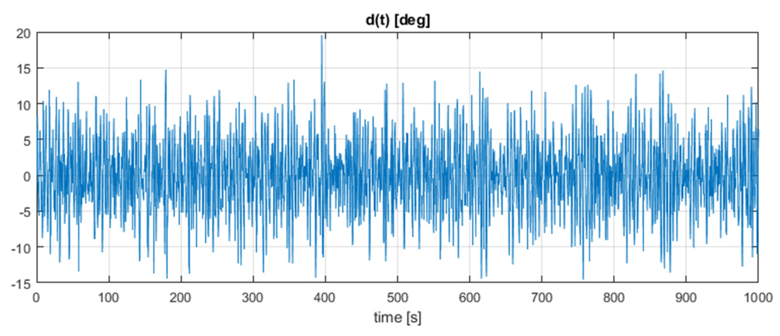
During the last test, a white noise generator with the sampling time and power parameter set as 0.5 s and 0.0001, respectively, was connected to a band-pass filter, described by the following transfer function [10,31]
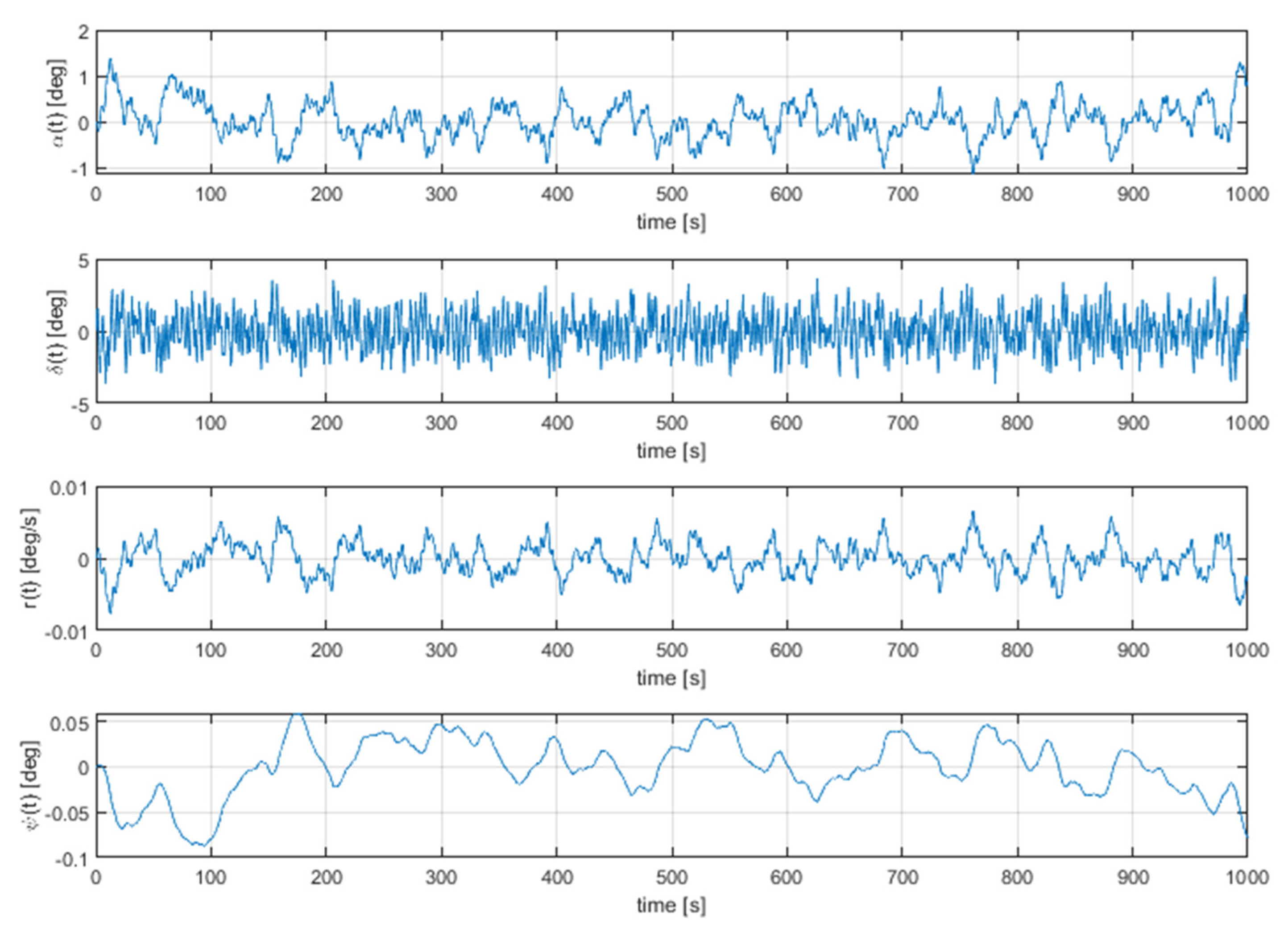
The obtained simulation results are presented in Figure 4 and Figure 5. The first shows variations of disturbance d(t) as coloured-noise, expressed in degrees, whereas in Figure 5 the heading angle vs. time is shown.
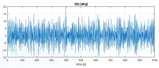
Figure 4.
Coloured-noise disturbance used in simulation.
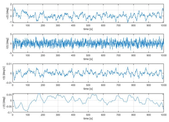
Figure 5.
Responses of the heading angle under the influence of the disturbance.
As can be seen, the course angle deviation values obtained are practically negligible. However, the robust response to random disturbances requires high performance of the steering gear machinery.
7. Discussion and Conclusions
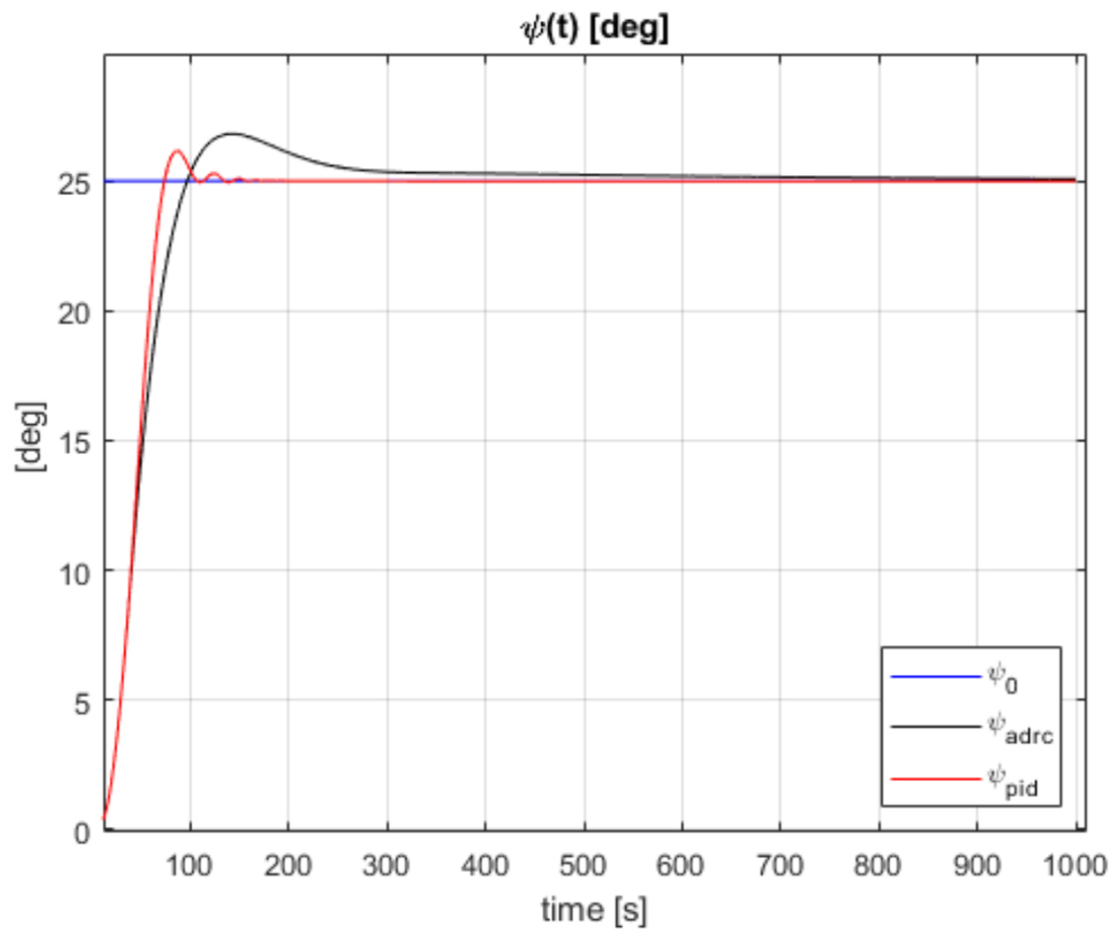
If we compare the above performance of ADRC to PID with laboratory, well-tuned controller parameters (in our case resolved to: Kp = 3.81, Kd = 3.95, Ki = 0.00547), then the transients, for the step disturbance, are shown in Figure 6.

Figure 6.
Comparison of ADRC to PID.
Differences in the response between ADRC and PID seem to be practically negligible, so that ADRC, in the conditions of our ship simulation model, proved to be similar in performance to PID.
However, it should be strongly emphasized that such a good tuning of the PID controller is not achievable in practice. From this point of view, and the fact of the simple, global tuning of the ADRC controller, there is no doubt that this controller performs much better.
Unfortunately, due to the research and development on ADRC for ship steering being at an early stage, and hence a significant lack of other reference data, especially for a more or less direct comparison and assessment of our ADRC results, we are not able to put them in a much wider context.
The ADRC autopilot tests carried out are very preliminary, but the results are already promising. The proposed system with the ADRC algorithm is characterized not only by robustness against the influence of constant and random disturbances but the first priority is the ease of its tuning, which is relatively simple.
We just need to know the parameter and the gains . However, for the estimation of , we proposed the formula (29), valid for a wide class of merchant vessels, while the gains can be easily determined by the general canonical model (6). This comes down to the choice of settling time (38) that can be rather arbitrarily performed under laboratory conditions. As shown in Figure 2, due to the robustness of this parameter, its nominal selection (the settling time 150 s) should ensure sufficiently good control performance for a real ship.
There is no doubt that the presented system requires further research. Important issues are, for example, its functioning with the introduced dead-band in order to reduce the intensity of the steering gear operation, or the issue of assessing its performance using integral quality indices (cf. [10]).
Nevertheless, the final evaluation of the system would require tests on a real ship, which, due to the fact that the simulation tests were carried out on a verified, full ship model, provides a chance that the implementation will work correctly.
Author Contributions
Conceptualization, Z.Z.; methodology, Z.Z. and J.A.; software, L.D.; validation, Z.Z. and J.A.; formal analysis, Z.Z. and J.A.; investigation, Z.Z.; writing—original draft preparation, Z.Z. and J.A.; writing—review and editing, Z.Z.; visualization, L.D.; supervision, Z.Z. All authors have read and agreed to the published version of the manuscript.
Funding
This research received no external funding.
Institutional Review Board Statement
Not applicable.
Informed Consent Statement
Not applicable.
Data Availability Statement
Not applicable.
Conflicts of Interest
The authors declare no conflict of interest. The funders had no role in the design of the study; in the collection, analyses, or interpretation of data; in the writing of the manuscript, or in the decision to publish the results.
Appendix A
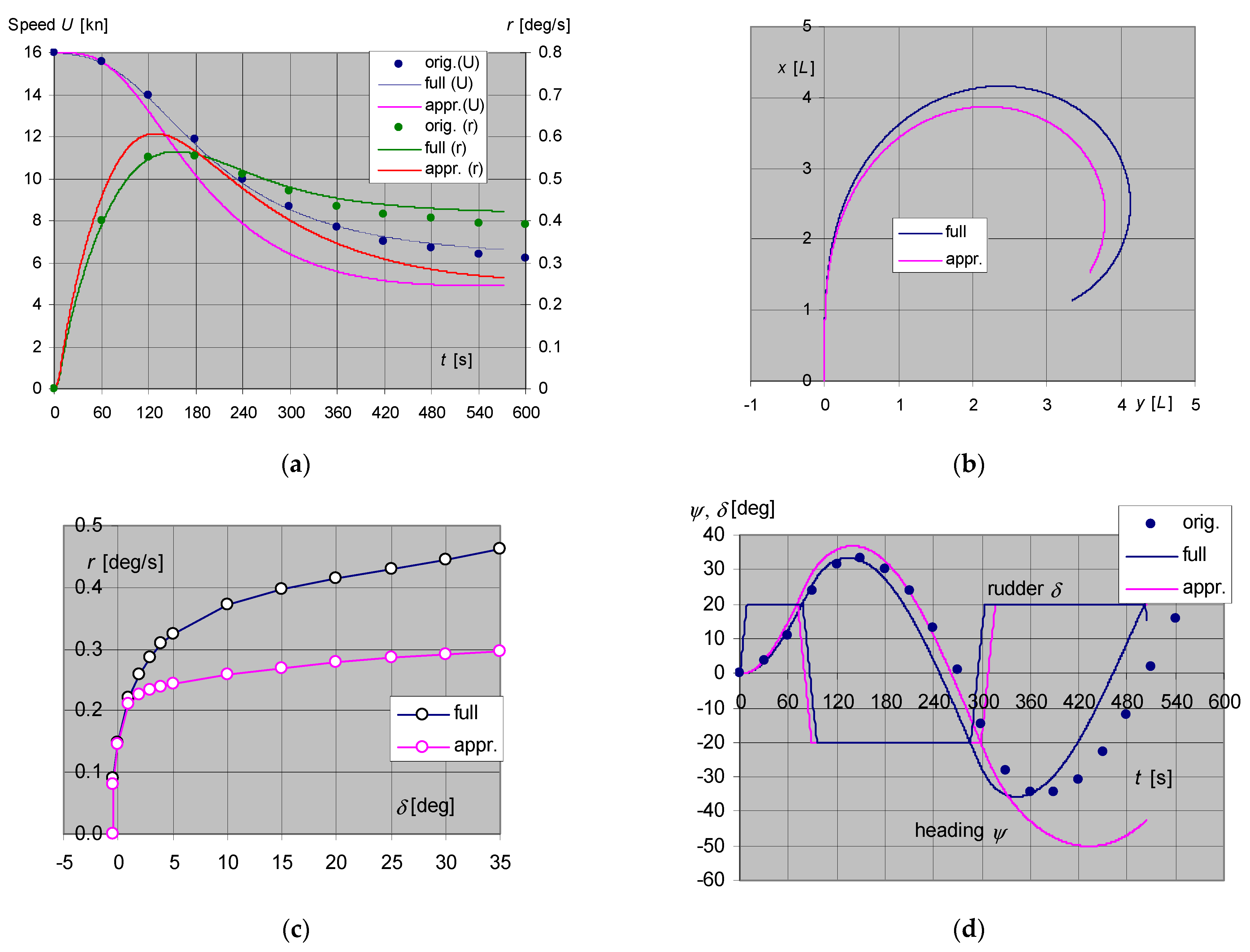
Figure A1 shows the performance of the model in Section 3.1, where a comparison is also made towards the original full model [23]. The symbol ‘orig.’ is used for the simulated data of [23], ‘full’ denotes the authors’ reproduction of this data with the full model of [22,23] as discussed in the paper, ‘appr.’ means the output of the proposed approximate model of Section 3.1 as developed by the authors, in particular of Table 2 as annotated.

Figure A1.
Selected standard manoeuvres of present ship model (with comparison towards original model: (a) turning circle test, 16 kn/20°, total linear speed (U) and rate of turn; (b) turning circle test, 16 kn/20°, trajectory x–y in ship’s length units; (c) spiral test at 16 kn; (d) Zig-zag test 20°/20° at 16 kn.
References
- Liu, Z.; Jin, H.; Grimble, M.J.; Katebi, R. Ship forward speed loss minimization using nonlinear course keeping and roll motion controllers. Ocean Eng. 2016, 113, 201–207. [Google Scholar] [CrossRef]
- Fossen, T. High Performance Ship Autopilot with Wave Filter. In Proceedings of the 10th Ship Control System Symposium (SCSS’ 1993), Ottawa, ON, Canada, 25–29 October 1993. [Google Scholar]
- Nguyen, T.-H.; Ha, T.-T.; Pham, H.-S.; Hoang, T.-H.; Giap, V.-D.; Le, T.-V. Study on an Effective Adaptive Ship Autopilot. In Proceedings of the SICE 2004 Annual Conference, Sapporo, Japan, 4–6 August 2004. [Google Scholar]
- Zwierzewicz, Z. On the Ship Course-Keeping Control System Design by Using Robust and Adaptive Control. In Proceedings of the 19th IEEE International Conference on Methods and Models in Automation and Robotics (MMAR), Międzyzdroje, Poland, 2–5 September 2014. [Google Scholar]
- Roberts, G.N.; Sutton, R.; Zirilli, A.; Tiano, A. Intelligent ship autopilots–A historical perspective. Mechatronics 2003, 13, 1091–1103. [Google Scholar] [CrossRef]
- Zhou, F.; Wang, C.; Li, F.; Ruan, J.; Pan, W. Nonlinear Active Disturbance Rejection Controller Research of Autopilot for Ship Course Tracking. In Proceedings of the 2008 Chinese Control and Decision Conference (CCDC 2008), Yantai, China, 2–4 July 2008. [Google Scholar] [CrossRef]
- Wang, J.; Wang, X.; Luo, Z.; Assadian, F. Active disturbance rejection control of differential drive assist steering for electric vehicles. Energies 2020, 13, 2647. [Google Scholar] [CrossRef]
- Witkowska, A.; Tomera, M.; Śmierzchalski, R. A backstepping approach to ship course control. Int. J. Appl. Math. Comput. Sci. 2007, 17, 73–85. [Google Scholar] [CrossRef] [Green Version]
- Casado, M.H.; Ferreiro, R. Identification of the nonlinear ship model parameters based on the turning test trial and the backstepping procedure. Ocean Eng. 2005, 32, 1350–1369. [Google Scholar] [CrossRef]
- Zwierzewicz, Z.; Dorobczyński, L.; Jaszczak, S. Design of Ship Course-Keeping System via Active Disturbance Rejection Control Using a Full-Scale Realistic Ship Model. Procedia Comput. Sci. 2021, 192, 3000–3009. [Google Scholar] [CrossRef]
- Tomera, M. Switching-Based Multi-Operational Control of Ship Motion; Academic Publishing House EXIT: Warsaw, Poland, 2018. [Google Scholar]
- Tomera, M. Track-keeping of a physical model of the tanker along a specified route. In Zeszyty Naukowe Wydziału Elektrotechniki i Automatyki PG; Scientific Journal of the Faculty of Electrical and Control Engineering, Gdansk University of Technology, Poland: Gdansk, Poland, 2016; ISSN 2353-1290. (In Polish) [Google Scholar]
- Von Ellenrieder, K.D. Control of Marine Vehicles; Springer: Cham, Switzerland, 2021. [Google Scholar]
- Astrom, K.J.; Hagglund, T. PID Controllers: Theory, Design, and Tuning, 2nd ed.; Instrument Society of America: Research Triangle Park, NC, USA, 1995. [Google Scholar]
- Kallstrom, C.G.; Norrbin, N.H. Performance Criteria for Ship Autopilots (An Analysis of Shipboard Experiments); Publication No. 9; SSPA: Goteborg, Sweden, 1984. [Google Scholar]
- Do, K.D. Practical control of underactuated ships. Ocean Eng. 2010, 37, 1111–1119. [Google Scholar] [CrossRef]
- Han, J. Active disturbance rejection controller and its applications. Control Decis. 1998, 13, 19–23. (In Chinese) [Google Scholar]
- Han, J. From PID to active disturbance rejection control. IEEE Trans. Ind. Electron. 2009, 56, 900–906. [Google Scholar] [CrossRef]
- Huang, Y.; Xue, W.; Gao, Z.; Sira-Ramirez, H.; Wu, D.; Sun, M. Active disturbance rejection control: Methodology, practice and analysis. In Proceedings of the 33rd Chinese Control Conference, Nanjing, China, 28–30 July 2014. [Google Scholar] [CrossRef]
- Guo, B.-Z.; Zhao, Z.-L. Active Disturbance Rejection Control for Nonlinear Systems: An Introduction; John Wiley & Sons: Singapore, 2016. [Google Scholar]
- De Larminat, P. (Ed.) Analysis and Control of Linear Systems; ISTE Ltd.: London, UK, 2007. [Google Scholar]
- Fossen, T. Guidance and Control of Ocean Vehicles; John Wiley & Sons: Chichester, UK, 1994. [Google Scholar]
- van Berlekom, W.B.; Goddard, T.A. Maneuvering of Large Tankers. Trans. SNAME 1972, 80, 264–298. [Google Scholar]
- Norrbin, N.H. Theory and Observations on the Use of a Mathematical Model for Ship Manoeuvring in Deep and Confined Waters; Publication No. 68; SSPA: Goteborg, Sweden, 1971. [Google Scholar]
- Kijima, K.; Tanaka, S.; Furukawa, Y.; Hori, T. On a Prediction Method of Ship Manoeuvring Characteristics. In Proceedings of the International Conference on Marine Simulation and Ship Manoeuvrability, MARSIM 93, St. John’s, NL, Canada, 26 September–2 October 1993; Volume 1. [Google Scholar]
- Liu, J.; Hekkenberg, R. Sixty years of research on ship rudders: Effects of design choices on rudder performance. Ships Offshore Struct. 2017, 12, 495–512. [Google Scholar] [CrossRef] [Green Version]
- Brix, J. (Ed.) Manoeuvring Technical Manual; Seehafen: Hamburg, Germany, 1993. [Google Scholar]
- Gofman, A.D. Propeller-Rudder System and Ship Manoeuvring (Handbook); Sudostroenie: Leningrad, Russia, 1988. (In Russian) [Google Scholar]
- Khalil, H.K. Nonlinear Systems, 3rd ed.; Prentice Hall: Upper Saddle River, NJ, USA, 2002; pp. 509–521. [Google Scholar]
- Herbst, G. A simulative study on Active Disturbance Rejection Control (ADRC) as a control tool for practitioners. Electronics 2013, 2, 246–279. [Google Scholar] [CrossRef]
- Lerner, D.M.; Lukomskiy, J.A.; Michailov, V.A.; Nornevskiy, B.I.; Petrov, J.P.; Popov, O.S.; Schleyer, G.E. Control of Marine Mobile Objects; Sudostroienie: Leningrad, Russia, 1979. (In Russian) [Google Scholar]
Publisher’s Note: MDPI stays neutral with regard to jurisdictional claims in published maps and institutional affiliations. |
© 2021 by the authors. Licensee MDPI, Basel, Switzerland. This article is an open access article distributed under the terms and conditions of the Creative Commons Attribution (CC BY) license (https://creativecommons.org/licenses/by/4.0/).