
ARIMA Models in Electrical Load Forecasting and Their Robustness to Noise


Abstract
:1. Introduction
- Development of studies on the impact of noise in time series on the forecasting model identifiability and their robustness,
- Assessment of the tolerance to noise of ARIMA models,
- Formulation of practical guidelines for the use of ARIMA models in noise laden electrical load forecasting.
2. ARIMA Models and Their Identification
- —coefficient at observation ,
- —error distributed as white noise,
- p—the order expresses the earliest value included,
- —coefficient at error ,
- q—the order of the series depends on the earliest previous error.
- —moving-average operator, represented as a polynomial in the backshift operator;
- —autoregressive operator, represented as a polynomial in the backshift operator.
- d—order of integration (differencing).
- —seasonal autoregressive operator,
- —seasonal moving-average operator.
- —first seasonal autoregressive operator,
- —first seasonal moving-average operator,
- —second seasonal autoregressive operator,
- —second seasonal moving-average operator.
- —numerator polynomial of the transfer function for the ith input series,
- —denominator polynomial of the transfer function for the ith input series,
- —the pure delay for effect of . at time t.
3. Background Literature
4. Research Methodology and Experiment Design
5. Simulation Results
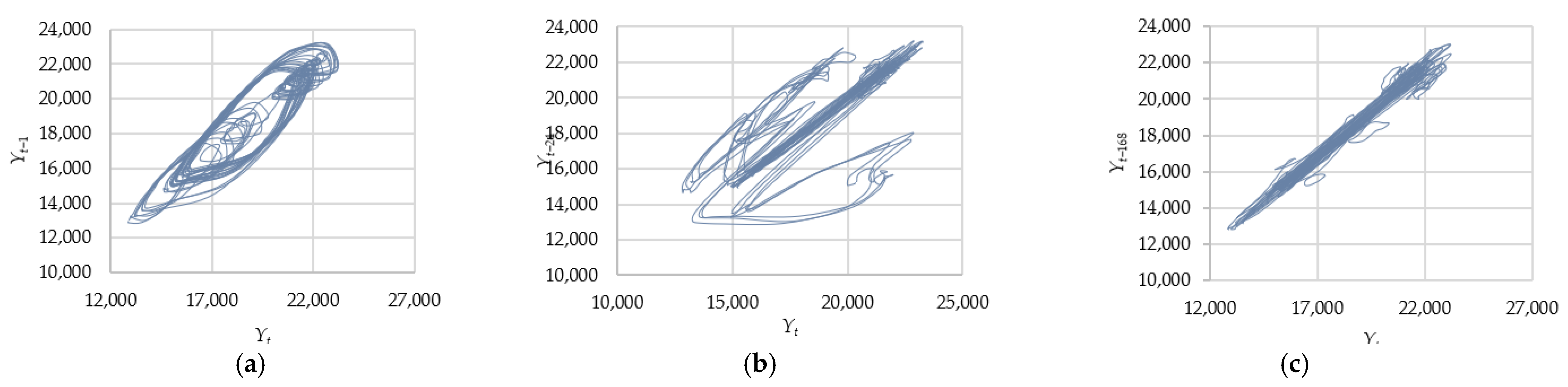
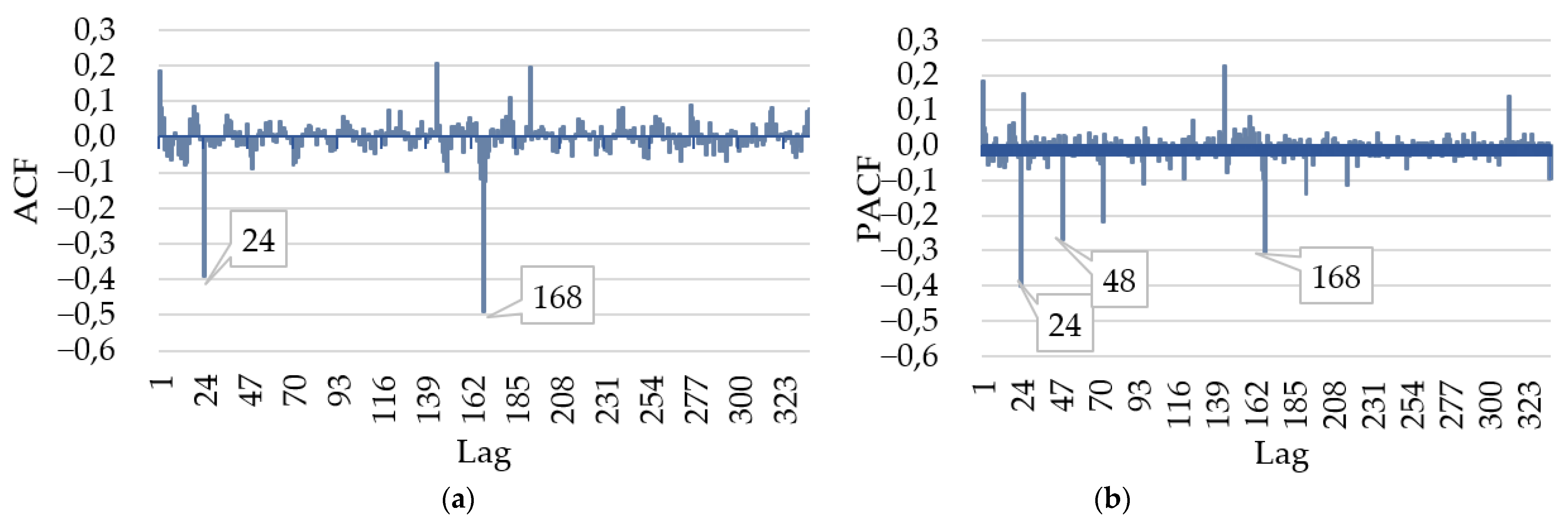
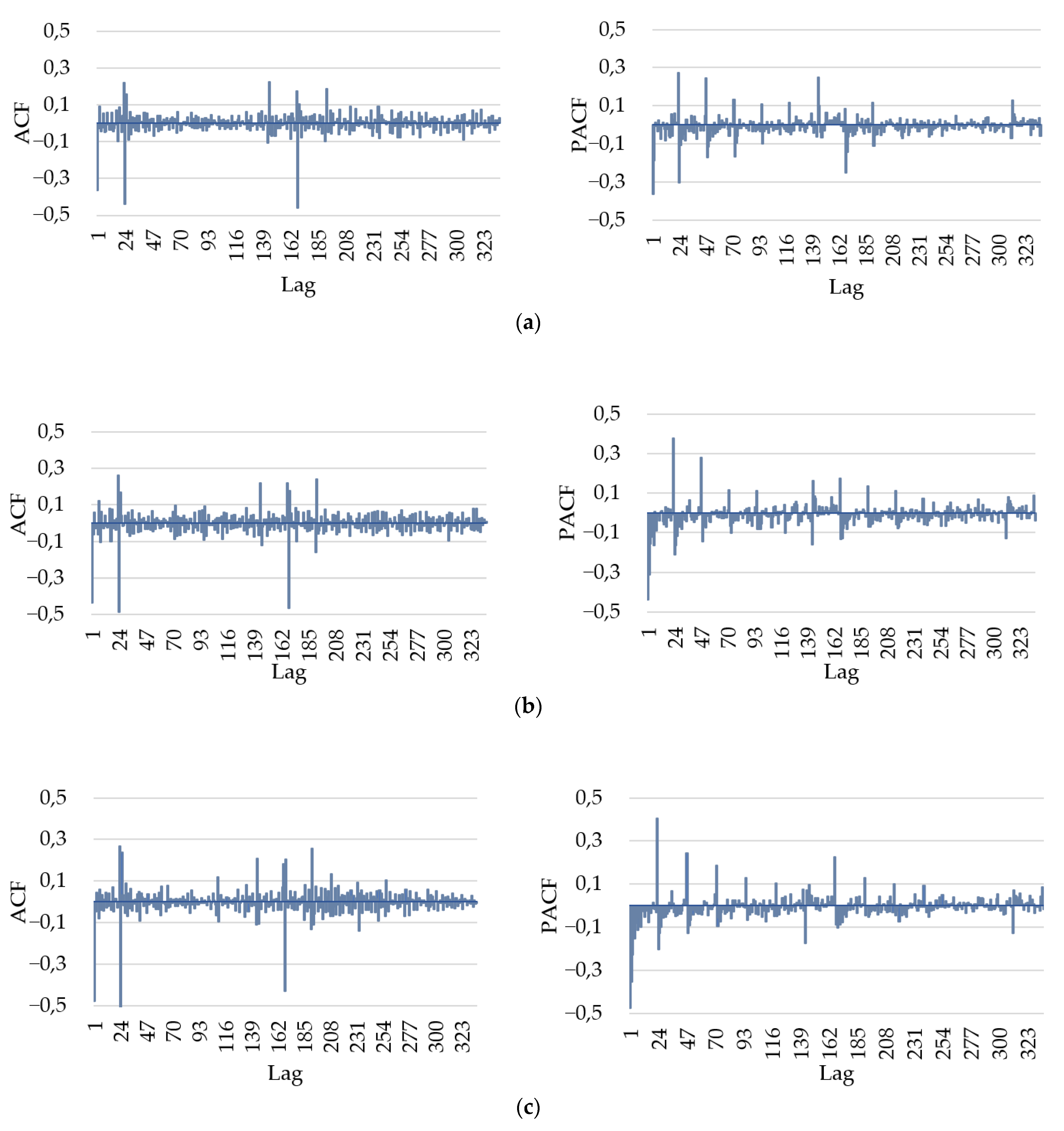
5.1. ARIMA Model Identification
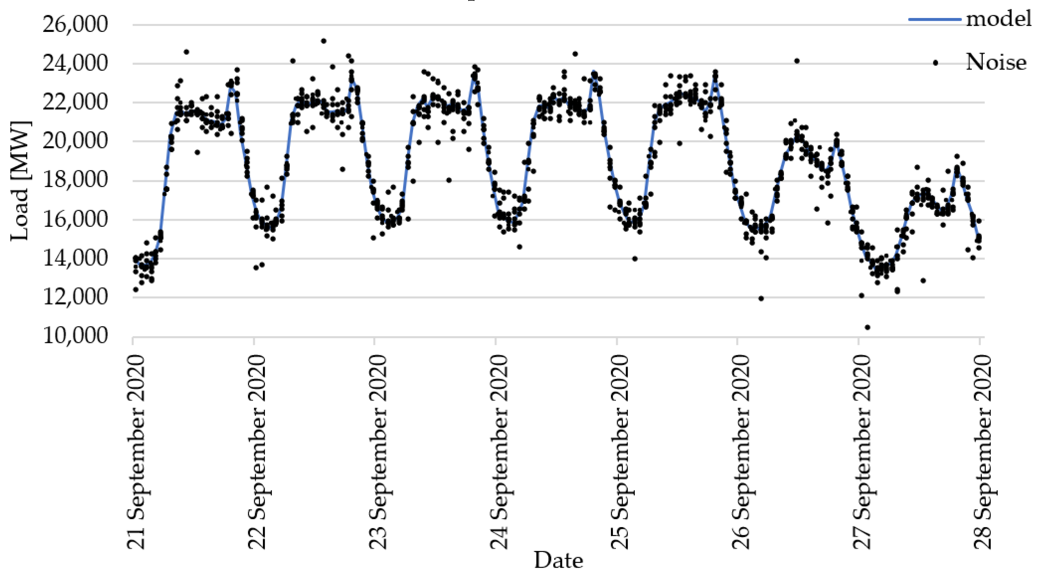
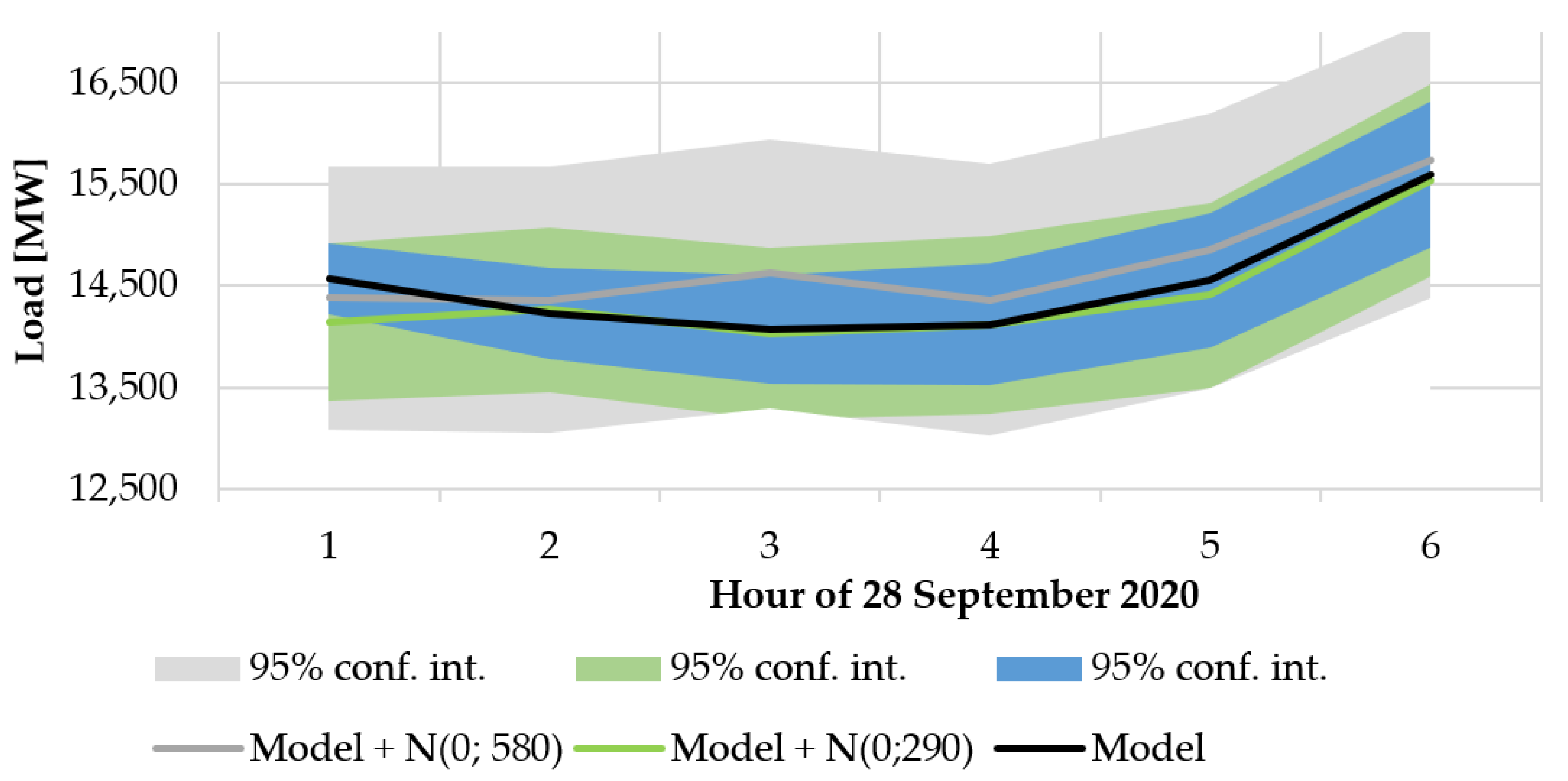
5.2. Simulation of the Impact of Random Noise
- —inference noise standard deviation,
- —signal standard deviation,
- NSR—noise to signal ratio.
6. Discussion
7. Conclusions
- Noise loading of the signal significantly affects the identification of the time series ARIMA model type and the estimation of its parameters,
- The accuracy of the prediction of electrical loads strongly depends on the noise level in the observed signal,
- The observed time series of the electrical load should be carefully examined for the presence and the level of noise in the signal before the prediction is performed,
- Usefulness of extending the classic Box–Jenkins approach by the preliminary time series filtration is proven.
Author Contributions
Funding
Institutional Review Board Statement
Informed Consent Statement
Data Availability Statement
Conflicts of Interest
References
- Soliman, S.A.; Alkandari, A.M. Electrical Load Forecasting: Modeling and Model Construction; Butterworth-Heinemann: Burlington, MA, USA, 2010; ISBN 978-0-12-381543-9. [Google Scholar]
- Nti, I.K.; Teimeh, M.; Nyarko-Boateng, O.; Adekoya, A.F. Electricity Load Forecasting: A Systematic Review. J. Electr. Syst. Inf Technol 2020, 7, 13. [Google Scholar] [CrossRef]
- Hammad, M.A.; Jereb, B.; Rosi, B.; Dragan, D. Methods and Models for Electric Load Forecasting: A Comprehensive Review. Logist. Sustain. Transp. 2020, 11, 51–76. [Google Scholar] [CrossRef] [Green Version]
- Hong, T.; Fan, S. Probabilistic Electric Load Forecasting: A Tutorial Review. Int. J. Forecast. 2016, 32, 914–938. [Google Scholar] [CrossRef]
- Hahn, H.; Meyer-Nieberg, S.; Pickl, S. Electric Load Forecasting Methods: Tools for Decision Making. Eur. J. Oper. Res. 2009, 199, 902–907. [Google Scholar] [CrossRef]
- Kuster, C.; Rezgui, Y.; Mourshed, M. Electrical Load Forecasting Models: A Critical Systematic Review. Sustain. Cities Soc. 2017, 35, 257–270. [Google Scholar] [CrossRef]
- Singh, S. Noise Impact on Time-Series Forecasting Using an Intelligent Pattern Matching Technique. Pattern Recognit. 1999, 32, 1389–1398. [Google Scholar] [CrossRef]
- Flores, J.J.; Calderon, F.; Cedeno Gonzalez, J.R.; Ortiz, J.; Farias, R.L. Comparison of Time Series Forecasting Techniques with Respect to Tolerance to Noise. In Proceedings of the 2016 IEEE International Autumn Meeting on Power, Electronics and Computing (ROPEC), Ixtapa, Mexico, 9–11 November 2016; IEEE: Piscataway, NJ, USA, 2016; pp. 1–6. [Google Scholar]
- Box, G.E.P.; Jenkins, G.M. Time Series Analysis: Forecasting and Control; Holden-Day series in time series analysis and digital processing; Rev. ed.; Holden-Day: San Francisco, CA, USA, 1976; ISBN 978-0-8162-1104-3. [Google Scholar]
- Rosadi, D. New Procedure for Determining Order of Subset Autoregressive Integrated Moving Average (ARIMA) Based on over-Fitting Concept. In Proceedings of the 2012 International Conference on Statistics in Science, Business and Engineering (ICSSBE), Langkawi, Kedah, Malaysia, 10–12 September 2012; IEEE: Piscataway, NJ, USA, 2012; pp. 1–5. [Google Scholar]
- Awan, T.M.; Aslam, F. Prediction of Daily COVID-19 Cases in European Countries Using Automatic ARIMA Model. J. Public Health Res. 2020, 9, 1765. [Google Scholar] [CrossRef]
- Villegas, M.A.; Pedregal, D.J. Automatic Selection of Unobserved Components Models for Supply Chain Forecasting. Int. J. Forecast. 2019, 35, 157–169. [Google Scholar] [CrossRef] [Green Version]
- Awe, O.; Okeyinka, A.; Fatokun, J.O. An Alternative Algorithm for ARIMA Model Selection. In Proceedings of the 2020 International Conference in Mathematics, Computer Engineering and Computer Science (ICMCECS), Lagos, Nigeria, 18–21 March 2020; IEEE: Piscataway, NJ, USA, 2020; pp. 1–4. [Google Scholar]
- Lénárt, B. Automatic Identification of ARIMA Models with Neural Network. Per. Pol. Transp. Eng. 2011, 39, 39. [Google Scholar] [CrossRef]
- Włodarczyk, A. X-13-ARIMA-SEATS as a Tool Supporting Environmental Management Process in the Power Plants. PJMS 2017, 16, 280–291. [Google Scholar] [CrossRef]
- Li, G.; Wang, Y. Automatic ARIMA Modeling-Based Data Aggregation Scheme in Wireless Sensor Networks. J. Wirel. Com. Netw. 2013, 2013, 85. [Google Scholar] [CrossRef]
- Caro, E.; Juan, J.; Cara, J. Periodically Correlated Models for Short-Term Electricity Load Forecasting. Appl. Math. Comput. 2020, 364, 124642. [Google Scholar] [CrossRef]
- Deb, C.; Zhang, F.; Yang, J.; Lee, S.E.; Shah, K.W. A Review on Time Series Forecasting Techniques for Building Energy Consumption. Renew. Sustain. Energy Rev. 2017, 74, 902–924. [Google Scholar] [CrossRef]
- Chodakowska, E.; Nazarko, J. Assessing the Performance of Sustainable Development Goals of EU Countries: Hard and Soft Data Integration. Energies 2020, 13, 3439. [Google Scholar] [CrossRef]
- Kao, Y.-S.; Nawata, K.; Huang, C.-Y. Predicting Primary Energy Consumption Using Hybrid ARIMA and GA-SVR Based on EEMD Decomposition. Mathematics 2020, 8, 1722. [Google Scholar] [CrossRef]
- Son, H.; Kim, Y.; Kim, S. Time Series Clustering of Electricity Demand for Industrial Areas on Smart Grid. Energies 2020, 13, 2377. [Google Scholar] [CrossRef]
- Trull, O.; García-Díaz, J.C.; Peiró-Signes, A. Forecasting Irregular Seasonal Power Consumption. An Application to a Hot-Dip Galvanizing Process. Appl. Sci. 2020, 11, 75. [Google Scholar] [CrossRef]
- Parsai, S.; Mahajan, S. Anomaly Detection Using Long Short-Term Memory. In Proceedings of the 2020 International Conference on Electronics and Sustainable Communication Systems (ICESC), Coimbatore, India, 2–4 July 2020; IEEE: Piscataway, NJ, USA, 2020; pp. 333–337. [Google Scholar]
- Lee, J.-W.; Kim, H.-J.; Kim, M.-K. Design of Short-Term Load Forecasting Based on ANN Using Bigdata. KIEE 2020, 69, 792–799. [Google Scholar] [CrossRef]
- Sáenz-Peñafiel, J.-J.; Luzuriaga, J.E.; Lemus-Zuñiga, L.-G.; Solis-Cabrera, V. A Comprehensive Solution for Electrical Energy Demand Prediction Based on Auto-Regressive Models. In Systems and Information Sciences; Botto-Tobar, M., Zamora, W., Larrea Plúa, J., Bazurto Roldan, J., Santamaría Philco, A., Eds.; Advances in Intelligent Systems and Computing; Springer International Publishing: Cham, Switzerland, 2021; Volume 1273, pp. 443–454. ISBN 978-3-030-59193-9. [Google Scholar]
- Nafil, A.; Bouzi, M.; Anoune, K.; Ettalabi, N. Comparative Study of Forecasting Methods for Energy Demand in Morocco. Energy Rep. 2020, 6, 523–536. [Google Scholar] [CrossRef]
- Sun, T.; Zhang, T.; Teng, Y.; Chen, Z.; Fang, J. Monthly Electricity Consumption Forecasting Method Based on X12 and STL Decomposition Model in an Integrated Energy System. Math. Probl. Eng. 2019, 2019, 1–16. [Google Scholar] [CrossRef]
- Han, X.; Li, R. Comparison of Forecasting Energy Consumption in East Africa Using the MGM, NMGM, MGM-ARIMA, and NMGM-ARIMA Model. Energies 2019, 12, 3278. [Google Scholar] [CrossRef] [Green Version]
- Borthakur, P.; Goswami, B. Short Term Load Forecasting: A Hybrid Approach Using Data Mining Methods. In Proceedings of the 2020 International Conference on Emerging Frontiers in Electrical and Electronic Technologies (ICEFEET), Patna, India, 10–11 July 2020; IEEE: Piscataway, NJ, USA, 2020; pp. 1–6. [Google Scholar]
- Bui, D.M.; Le, P.D.; Cao, M.T.; Pham, T.T.; Pham, D.A. Accuracy Improvement of Various Short-Term Load Forecasting Models by a Novel and Unified Statistical Data-Filtering Method. Int. J. Green Energy 2020, 17, 382–406. [Google Scholar] [CrossRef]
- Jahanshahi, A.; Jahanianfard, D.; Mostafaie, A.; Kamali, M. An Auto Regressive Integrated Moving Average (ARIMA) Model for Prediction of Energy Consumption by Household Sector in Euro Area. AIMS Energy 2019, 7, 151–164. [Google Scholar] [CrossRef]
- Noureen, S.; Atique, S.; Roy, V.; Bayne, S. Analysis and Application of Seasonal ARIMA Model in Energy Demand Forecasting: A Case Study of Small Scale Agricultural Load. In Proceedings of the 2019 IEEE 62nd International Midwest Symposium on Circuits and Systems (MWSCAS), Dallas, TX, USA, 4–7 August 2019; IEEE: Piscataway, NJ, USA, 2019; pp. 521–524. [Google Scholar]
- Salam, M.A.; Yazdani, M.G.; Wen, F.; Rahman, Q.M.; Malik, O.A.; Hasan, S. Modeling and Forecasting of Energy Demands for Household Applications. Glob. Chall. 2020, 4, 1900065. [Google Scholar] [CrossRef] [PubMed]
- Luan, C.; Pang, X.; Wang, Y.; Liu, L.; You, S. Comprehensive Forecasting Method of Monthly Electricity Consumption Based on Time Series Decomposition and Regression Analysis. In Proceedings of the 2020 2nd International Conference on Industrial Artificial Intelligence (IAI), Shenyang, China, 24–26 July 2020; IEEE: Piscataway, NJ, USA, 2020; pp. 1–6. [Google Scholar]
- 3Mehedintu, A.; Sterpu, M.; Soava, G. Estimation and Forecasts for the Share of Renewable Energy Consumption in Final Energy Consumption by 2020 in the European Union. Sustainability 2018, 10, 1515. [Google Scholar] [CrossRef] [Green Version]
- Méndez-Gordillo, A.R.; Cadenas, E. Wind Speed Forecasting by the Extraction of the Multifractal Patterns of Time Series through the Multiplicative Cascade Technique. Chaos Solitons Fractals 2021, 143, 110592. [Google Scholar] [CrossRef]
- Marulanda, G.; Bello, A.; Cifuentes, J.; Reneses, J. Wind Power Long-Term Scenario Generation Considering Spatial-Temporal Dependencies in Coupled Electricity Markets. Energies 2020, 13, 3427. [Google Scholar] [CrossRef]
- Bórawski, P.; Bełdycka-Bórawska, A.; Jankowski, K.J.; Dubis, B.; Dunn, J.W. Development of Wind Energy Market in the European Union. Renew. Energy 2020, 161, 691–700. [Google Scholar] [CrossRef]
- Lei, Y.; Xue, P.; Li, Y. Comparison of Holt-Winters and ARIMA Models for Hydropower Forecasting in Guangxi. In Proceedings of the Proceedings of the 2020 3rd International Conference on Signal Processing and Machine Learning, Beijing, China, 22–24 October 2020; ACM: New York, NY, USA, 2020; pp. 63–67. [Google Scholar]
- Jamil, R. Hydroelectricity Consumption Forecast for Pakistan Using ARIMA Modeling and Supply-Demand Analysis for the Year 2030. Renew. Energy 2020, 154, 1–10. [Google Scholar] [CrossRef]
- Barzola-Monteses, J.; Mite-León, M.; Espinoza-Andaluz, M.; Gómez-Romero, J.; Fajardo, W. Time Series Analysis for Predicting Hydroelectric Power Production: The Ecuador Case. Sustainability 2019, 11, 6539. [Google Scholar] [CrossRef] [Green Version]
- Belmahdi, B.; Louzazni, M.; Bouardi, A.E. One Month-Ahead Forecasting of Mean Daily Global Solar Radiation Using Time Series Models. Optik 2020, 219, 165207. [Google Scholar] [CrossRef]
- 4Lu, Y.-S.; Lai, K.-Y. Deep-Learning-Based Power Generation Forecasting of Thermal Energy Conversion. Entropy 2020, 22, 1161. [Google Scholar] [CrossRef]
- Dittmer, C.; Krümpel, J.; Lemmer, A. Power Demand Forecasting for Demand-Driven Energy Production with Biogas Plants. Renew. Energy 2021, 163, 1871–1877. [Google Scholar] [CrossRef]
- Leerbeck, K.; Bacher, P.; Junker, R.G.; Goranović, G.; Corradi, O.; Ebrahimy, R.; Tveit, A.; Madsen, H. Short-Term Forecasting of CO2 Emission Intensity in Power Grids by Machine Learning. Appl. Energy 2020, 277, 115527. [Google Scholar] [CrossRef]
- Wang, Q.; Li, S.; Pisarenko, Z. Modeling Carbon Emission Trajectory of China, US and India. J. Clean. Prod. 2020, 258, 120723. [Google Scholar] [CrossRef]
- Malik, A.; Hussain, E.; Baig, S.; Khokhar, M.F. Forecasting CO2 Emissions from Energy Consumption in Pakistan under Different Scenarios: The China–Pakistan Economic Corridor. Greenh. Gas Sci. Technol. 2020, 10, 380–389. [Google Scholar] [CrossRef]
- Peshkov, A.V.; Alsova, O.K. Short-Term Forecasting of the Time Series of Electricity Prices with Ensemble Algorithms. J. Phys. Conf. Ser. 2020, 1661, 012070. [Google Scholar] [CrossRef]
- Nametala, C.; de Faria, W.; Junior, B. A Volatility Index for Bilateral Electricity Contracting Auctions. IEEE Lat. Am. Trans. 2020, 18, 938–946. [Google Scholar] [CrossRef]
- Nop, P.; Qin, Z. Cambodia Mid-Term Transmission System Load Forecasting with the Combination of Seasonal ARIMA and Gaussian Process Regression. In Proceedings of the 2021 3rd Asia Energy and Electrical Engineering Symposium (AEEES), Chengdu, China, 26–29 March 2021; IEEE: Piscataway, NJ, USA, 2021; pp. 700–707. [Google Scholar]
- Mpawenimana, I.; Pegatoquet, A.; Roy, V.; Rodriguez, L.; Belleudy, C. A Comparative Study of LSTM and ARIMA for Energy Load Prediction with Enhanced Data Preprocessing. In Proceedings of the 2020 IEEE Sensors Applications Symposium (SAS), Kuala Lumpur, Malaysia, 28–31 March 2020; IEEE: Piscataway, NJ, USA, 2020; pp. 1–6. [Google Scholar]
- Goswami, K.; Kandali, A.B. Electricity Demand Prediction Using Data Driven Forecasting Scheme: ARIMA and SARIMA for Real-Time Load Data of Assam. In Proceedings of the 2020 International Conference on Computational Performance Evaluation (ComPE), Shillong, India, 2–4 July 2020; IEEE: Piscataway, NJ, USA, 2020; pp. 570–574. [Google Scholar]
- Gupta, A.; Kumar, A. Mid Term Daily Load Forecasting Using ARIMA, Wavelet-ARIMA and Machine Learning. In Proceedings of the 2020 IEEE International Conference on Environment and Electrical Engineering and 2020 IEEE Industrial and Commercial Power Systems Europe (EEEIC/I&CPS Europe), Madrid, Spain, 9–12 June 2020; IEEE: Piscataway, NJ, USA, 2020; pp. 1–5. [Google Scholar]
- Wang, Y.; Zhang, W.; Li, X.; Wang, A.; Wu, T.; Bao, Y. Monthly Load Forecasting Based on an ARIMA-BP Model: A Case Study on Shaoxing City. In Proceedings of the 2020 12th IEEE PES Asia-Pacific Power and Energy Engineering Conference (APPEEC), Nanjing, China, 14–16 September 2020; IEEE: Piscataway, NJ, USA, 2020; pp. 1–6. [Google Scholar]
- Dinata, S.A.W.; Azka, M.; Faisal, M.; Suhartono; Yendra, R.; Gamal, M.D.H. Short-Term Load Forecasting Double Seasonal ARIMA Methods: An Evaluation Based on Mahakam-East Kalimantan Data. In Proceedings of the AIP Conference, Pontianak, Indonesia, 23–25 September 2020; p. 020004. [Google Scholar] [CrossRef]
- Yang, L.; Yang, H. A Combined ARIMA-PPR Model for Short-Term Load Forecasting. In Proceedings of the 2019 IEEE Innovative Smart Grid Technologies—Asia (ISGT) Asia, Chengdu, China, 21–24 May 2019; IEEE: Piscataway, NJ, USA, 2019; pp. 3363–3367. [Google Scholar]
- Yu, K.W.; Hsu, C.H.; Yang, S.M. A Model Integrating ARIMA and ANN with Seasonal and Periodic Characteristics for Forecasting Electricity Load Dynamics in a State. In Proceedings of the 2019 IEEE 6th International Conference on Energy Smart Systems (ESS), Kyiv, Ukraine, 17–19 April 2019; IEEE: Piscataway, NJ, USA, 2019; pp. 19–24. [Google Scholar]
- Tang, L.; Yi, Y.; Peng, Y. An Ensemble Deep Learning Model for Short-Term Load Forecasting Based on ARIMA and LSTM. In Proceedings of the 2019 IEEE International Conference on Communications, Control, and Computing Technologies for Smart Grids (SmartGridComm), Beijing, China, 21–23 October 2019; IEEE: Piscataway, NJ, USA, 2019; pp. 1–6. [Google Scholar]
- Amin, M.A.A.; Hoque, M.A. Comparison of ARIMA and SVM for Short-Term Load Forecasting. In Proceedings of the 2019 9th Annual Information Technology, Electromechanical Engineering and Microelectronics Conference (IEMECON), Jaipur, India, 13–15 March 2019; IEEE: Piscataway, NJ, USA, 2019; pp. 1–6. [Google Scholar]
- Zou, Z.; Wu, X.; Zhao, Z.; Wang, Q.; Bie, Y.; Zhou, M. Prediction of Short Term Electric Load Based on BP Neural Networks & ARIMA Combination. In Proceedings of the 2018 IEEE 4th Information Technology and Mechatronics Engineering Conference (ITOEC), Chongqing, China, 14–16 December 2018; IEEE: Piscataway, NJ, USA, 2018; pp. 1671–1674. [Google Scholar]
- Eljazzar, M.M.; Hemayed, E.E. Enhancing Electric Load Forecasting of ARIMA and ANN Using Adaptive Fourier Series. In Proceedings of the 2017 IEEE 7th Annual Computing and Communication Workshop and Conference (CCWC), Las Vegas, NV, USA, 9–11January 2017; IEEE: Piscataway, NJ, USA, 2017; pp. 1–6. [Google Scholar]
- Karthika, S.; Margaret, V.; Balaraman, K. Hybrid Short Term Load Forecasting Using ARIMA-SVM. In Proceedings of the 2017 Innovations in Power and Advanced Computing Technologies (i-PACT), Vellore, India, 21–22 April 2017; IEEE: Piscataway, NJ, USA, 2017; pp. 1–7. [Google Scholar]
- Khuntia, S.R.; Rueda, J.L.; van der Meijden, M.A.M.M. Volatility in Electrical Load Forecasting for Long-Term Horizon—An ARIMA-GARCH Approach. In Proceedings of the 2016 International Conference on Probabilistic Methods Applied to Power Systems (PMAPS), Beijing, China, 16–20 October 2016; IEEE: Piscataway, NJ, USA, 2016; pp. 1–6. [Google Scholar]
- Puspitasari, I.; Akbar, M.S.; Lee, M.H. Two-Level Seasonal Model Based on Hybrid ARIMA-ANFIS for Forecasting Short-Term Electricity Load in Indonesia. In Proceedings of the 2012 International Conference on Statistics in Science, Business and Engineering (ICSSBE), Langkawi, Kedah, Malaysia, 10–12 September 2012; IEEE: Piscataway, NJ, USA, 2012; pp. 1–5. [Google Scholar]
- Wei, L.; Zhen-gang, Z. Based on Time Sequence of ARIMA Model in the Application of Short-Term Electricity Load Forecasting. In Proceedings of the 2009 International Conference on Research Challenges in Computer Science, Shanghai, China, 28–29 December 2009; IEEE: Piscataway, NJ, USA, 2009; pp. 11–14. [Google Scholar]
- de Andrade, L.C.M.; da Silva, I.N. Very Short-Term Load Forecasting Based on ARIMA Model and Intelligent Systems. In Proceedings of the 2009 15th International Conference on Intelligent System Applications to Power Systems, Curitiba, Brazil, 8–12 November 2009; IEEE: Piscataway, NJ, USA, 2009; pp. 1–6. [Google Scholar]
- Hor, C.-L.; Watson, S.J.; Majithia, S. Daily Load Forecasting and Maximum Demand Estimation Using ARIMA and GARCH. In Proceedings of the 2006 International Conference on Probabilistic Methods Applied to Power Systems, Stockholm, Sweden, 11–15 June 2006; IEEE: Piscataway, NJ, USA, 2006; pp. 1–6. [Google Scholar]
- He, Y.; Zhu, Y.; Duan, D. Research on Hybrid ARIMA and Support Vector Machine Model in Short Term Load Forecasting. In Proceedings of the Sixth International Conference on Intelligent Systems Design and Applications, Jinan, China, 16–18 October 2006; IEEE: Jinan, China, 2006; Volume 1, pp. 804–809. [Google Scholar]
- Nazarko, J.; Jurczuk, A.; Zalewski, W. ARIMA Models in Load Modelling with Clustering Approach. In Proceedings of the 2005 IEEE Russia Power Tech, St. Petersburg, Russia, 27–30 June 2005; IEEE: Piscataway, NJ, USA, 2005; pp. 1–6. [Google Scholar]
- Lu, J.C.; Niu, D.X.; Jia, Z.Y. A Study of Short-Term Load Forecasting Based on ARIMA-ANN. In Proceedings of the Proceedings of 2004 International Conference on Machine Learning and Cybernetics (IEEE Cat. No.04EX826), Shanghai, China, 26–29 August 2004; IEEE: Piscataway, NJ, USA, 2004; pp. 3183–3187. [Google Scholar]
- Juberias, G.; Yunta, R.; Garcia Moreno, J.; Mendivil, C. A New ARIMA Model for Hourly Load Forecasting. In Proceedings of the 1999 IEEE Transmission and Distribution Conference (Cat. No. 99CH36333), New Orleans, LA, USA, 11–16 April 1999; IEEE: Piscataway, NJ, USA, 1999; Volume 1, pp. 314–319. [Google Scholar]
- Cho, M.Y.; Hwang, J.C.; Chen, C.S. Customer Short Term Load Forecasting by Using ARIMA Transfer Function Model. In Proceedings of the 1995 International Conference on Energy Management and Power Delivery EMPD ’95, Singapore, 21–23 November 1995; IEEE: Piscataway, NJ, USA, 1995; Volume 1, pp. 317–322. [Google Scholar]
- Voss, H.U.; Horbelt, W.; Timmer, J. Continuous Nonlinear Delayed-Feedback Dynamics from Noisy Observations. In Proceedings of the AIP Conference Proceedings, Albuquerque, New Mexico, 23–28 June 2002; AIP: Potsdam, Germany, 2002; Volume 622, pp. 163–173. [Google Scholar]
- Cellucci, C.J.; Albano, A.M.; Rapp, P.E.; Pittenger, R.A.; Josiassen, R.C. Detecting Noise in a Time Series. Chaos 1997, 7, 414–422. [Google Scholar] [CrossRef] [PubMed]
- Cao, M.T.; Pham, T.T.; Kuo, T.C.; Bui, D.M.; Nguyen, H.V.; Nguyen, T.H. Short-Term Load Forecasting Enhanced With Statistical Data-Filtering Method. In Proceedings of the 2020 IEEE International Conference on Power Electronics, Smart Grid and Renewable Energy (PESGRE2020), Cochin, India, 2–4 January 2020; IEEE: Piscataway, NJ, USA, 2020; pp. 1–8. [Google Scholar]
- Akdi, Y.; Dickey, D.A. Pfriodograms of Unit Root Time Series: Distributions and Tests. Commun. Stat.-Theory Methods 1998, 27, 69–87. [Google Scholar] [CrossRef]
- Pérez-Chacón, R.; Luna-Romera, J.; Troncoso, A.; Martínez-Álvarez, F.; Riquelme, J. Big Data Analytics for Discovering Electricity Consumption Patterns in Smart Cities. Energies 2018, 11, 683. [Google Scholar] [CrossRef] [Green Version]
- Noussan, M.; Roberto, R.; Nastasi, B. Performance Indicators of Electricity Generation at Country Level—The Case of Italy. Energies 2018, 11, 650. [Google Scholar] [CrossRef] [Green Version]
- Yao, W.; Essex, C.; Yu, P.; Davison, M. Measure of Predictability. Phys. Rev. E 2004, 69, 066121. [Google Scholar] [CrossRef] [PubMed] [Green Version]
- Gambuzza, L.V.; Buscarino, A.; Fortuna, L.; Porfiri, M.; Frasca, M. Analysis of Dynamical Robustness to Noise in Power Grids. IEEE J. Emerg. Sel. Top. Circuits Syst. 2017, 7, 413–421. [Google Scholar] [CrossRef]
- Cheba, K.; Bąk, I. Environmental Production Efficiency in the European Union Countries as a Tool for the Implementation of Goal 7 of the 2030 Agenda. Energies 2021, 14, 4593. [Google Scholar] [CrossRef]

| Abbreviation | Meaning |
|---|---|
| ACF | Autocorrelation Functions |
| AIC | Akaike Information Criterium |
| ANN | Artificial Neural Network |
| AR | Auto-Regressive |
| ARCH | Auto-Regressive Conditional Heteroskedasticity |
| ARFIMA | Fractionally Integrated ARMA |
| AR-GARCH | AR Models with GARCH Residuals |
| ARIMA | Auto-Regressive Integrated Moving Average |
| ARIMAX | Auto-Regressive Integrated Moving Average with Exogenous Variable |
| ARMA | Auto-Regressive and Moving Average |
| BIC | Bayesian Information Criteria |
| ESM | Exponential Smoothing Models |
| FARIMA | ARFIMA |
| FPE | Final Prediction Error |
| FRM | Fuzzy Regression Models |
| GARCH | Generalized Auto-Regressive Conditional Heteroskedasticity |
| LTLF | Long-Term Load Forecasting |
| MA | Moving Average |
| MAE | Mean Absolute Error |
| MAPE | Mean Absolute Percentage Error |
| MLR | Multiple Linear Regression |
| MTLF | Medium-Term Load Forecasting |
| MW | Megawatt |
| NSR | Noise to Signal Ratio |
| PACF | Partial Autocorrelation Functions |
| SARIMA | Seasonal Auto-Regressive Integrated Moving Average |
| STLF | Short-Term Load Forecasting |
| SVM | Support Vector Machines |
| VARMA | Vector ARIMA |
| VSTLF | Very Short-Term Load Forecasting |
| No | Year | Data/Forecast | ARIMA Model | Publications |
|---|---|---|---|---|
| 1 | 2021 | 10-year monthly load, Electricité Du Cambodge, Cambodia | ARIMA(2,0,2)(4,0,2)12 | Nop and Qin [50] |
| Multi-step, monthly load one-year ahead | ||||
| 2 | 2020 | 47-month daily load of household, France | ARIMA(1,0,2) | Mpawenimana et al. [51] |
| Multi-step, daily load 7, 14, 28, and 31 days ahead | ||||
| 3 | 2020 | 3-year daily 10 a.m. load, SLDC, Assam |
| Goswami and Kandali [52] |
| Multi-step, daily 10 a.m. load one-year ahead | ||||
| 4 | 2020 | 10-year daily load, Karnataka, India | Twelve models, each for a certain month January ARIMA(8,1,1) February ARIMA(5,4,1) March ARIMA(9,1,1) April ARIMA(5,5,1) May ARIMA(1,6,1) June ARIMA(4,3,1) July ARIMA(3,3,1) August ARIMA(8,2,1) September ARIMA(3,3,1) October ARIMA(2,6,1) November ARIMA(9,1,1) December ARIMA(5,3,1) | Gupta and Kumar [53] |
| Multi-step, daily load month-wise one-year ahead | ||||
| 5 | 2020 | 10-year monthly load, Shaoxing, China | ARIMA(12,2,9) | Wang et al. [54] |
| Multi-step, monthly load one-year ahead | ||||
| 6 | 2020 | 1-year hourly load, Mahakam East Kalimantan, Indonesia | ARIMA (0,1,1)(0,1,1)24(0,1,1)336 | Dinata et al. [55] |
| One-step, hourly load from one-week to one-month ahead Multi-step, hourly load from one-week to one-month ahead | ||||
| 7 | 2019 | 3-day 5 min interval load, Sichuan Province, China | ARIMA(2,2) | Yang and Yang [56] |
| Multi-step, 5 min load 30 min ahead for one day | ||||
| 8 | 2019 | 126-weak daily load, Taiwan Power Company, Taiwan | ARIMA(1,1,1)(1,1,1)7 | Yu, Hsu and Yang [57] |
| Daily load one-day ahead Multi-step, daily load one-week ahead | ||||
| 9 | 2019 | 3-year daily load, agriculture, PG&E, US | ARIMA(0,1,0)(1,1,1)12 | Noureen et al. [32] |
| Multi-step, monthly load one-year ahead | ||||
| 10 | 2019 | 14-year daily load, Toronto Canada | General model (a) ARIMA(2,0,8) Seven models, each for a certain day of week (b): Mon ARIMA(0,1,10); Tue ARIMA(0,1,10); Wed ARIMA(0,1,12); Thu ARIMA(0,1,10); Fri ARIMA(0,1,9); Sat ARIMA(0,1,10); Sun ARIMA(0,1,9) | Tang, Yi and Peng [58] |
| Multi-step, daily load one-week ahead | ||||
| 11 | 2019 | 3-month 15 min load, Builders Temporary Supply | ARIMA(2,1,1) | Amin and Hoque [59] |
| Multi-step, 15 min load one day ahead | ||||
| 12 | 2018 | One-week 15 min load, Shiqu, Ganzi State, China | ARIMA(13,1,15) | Zou et al. [60] |
| Multi-step 15 min load 12 h ahead | ||||
| 13 | 2017 | N/A | The most commonly used seasonal ARIMA is probably the ARIMA(0,1,1)(0,1,1) | Kuster, Rezgui, and Mourshed [6] |
| N/A | ||||
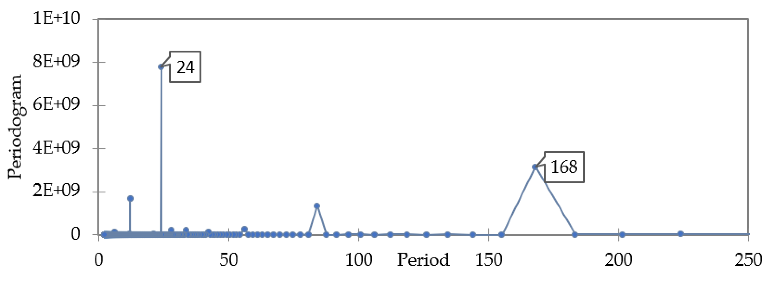
| 14 | 2017 | 2-year hourly peak load, TX, US | Three seasonal periods are defined as 24, 168, and 8766 for daily, weekly, and annually effect respectively | Eljazzar and Hemayed [61] |
| Multi-step, hourly peak load two years ahead | ||||
| 15 | 2017 | 2-year hourly load, southern region, India | ARIMA(4,0,1)24(2,1,2)168 | Karthika, Margaret, and Balaraman [62] |
| Multi-step, hourly load one day ahead | ||||
| 16 | 2016 | 20-year monthly load, Regional Transmission Organization, US | ARIMA(1,1,1) | Khuntia, Rueda, and van der Meijden [63] |
| Multi-step, monthly load one year ahead | ||||
| 17 | 2012 | 2-year half-hourly load, Java-Bali Indonesia | ARIMA(0,1,1)(0,1,1)7 | Suhartono et al. [64] |
| Multi-step, half-hourly load two weeks ahead separately for each half-hour of a day | ||||
| 18 | 2009 | 6-year monthly load data, China | ARIMA(4,1,4) | Wei and Zhen-gang [65] |
| Multi-step, monthly load six months ahead | ||||
| 19 | 2009 | One-week, 5 min load, substations located at Andradina, Ubatuba, and Votuporanga, Brazil | ARIMA(3,2,2)(0,1,1)12 ARIMA(4,2,2)(0,1,1)12 ARIMA(3,2,2)(0,1,1)12 | de Andrade and da Silva [66] |
| Multi-step, 5 min load twelve steps ahead | ||||
| 20 | 2006 | 33-year daily load, UK | ARIMIA(1,1,1) | Hor, Watson, and Majithia [67] |
| Multi-step, daily load four years ahead | ||||
| 21 | 2006 | 1-year 15 min load, Hebei province, China | ARIMA(2,2,3) | He, Zhu, and Duan [68] |
| Multi-step, 15 min load one day ahead | ||||
| 22 | 2005 | 2-month 15 min load of distribution substations, Bialystok, Poland | ARIMA(0,1,1)(0,1,1)96 | Nazarko Jurczuk, and Zalewski [69] |
| Daily load profile modelling | ||||
| 23 | 2004 | 1-year 15 min load, Hebei area, China | ARIMA(2,2,3) | Ran-chang Lu et al. [70] |
| Multi-step, 15 min load one day ahead | ||||
| 24 | 1999 | 6-month 1 h load series, Red Electrica de Espana, Spain | Logarithmic transformation ARIMA(1,1,0)(1,1,1)24(0,1,1)168 | Juberias et al. [71] |
| Multi-step, hourly load one day ahead | ||||
| 25 | 1995 | 1-year 5 min, Taipower, Taiwan | Commercial load ARIMA(1,0,0)(2,1,1)24 Office load ARIMA(2,0,0)(1,0,0)168(0,1,1)24 Industrial load, logarithmic transformation ARIMA(1,0,2) Residential load, logarithmic transformation ARIMA([1,4,5],00)(0,1,1)24 | Cho, Hwang, and Chen [72] |
| Multi-step, hourly load one week ahead |
| Characteristic | Value |
|---|---|
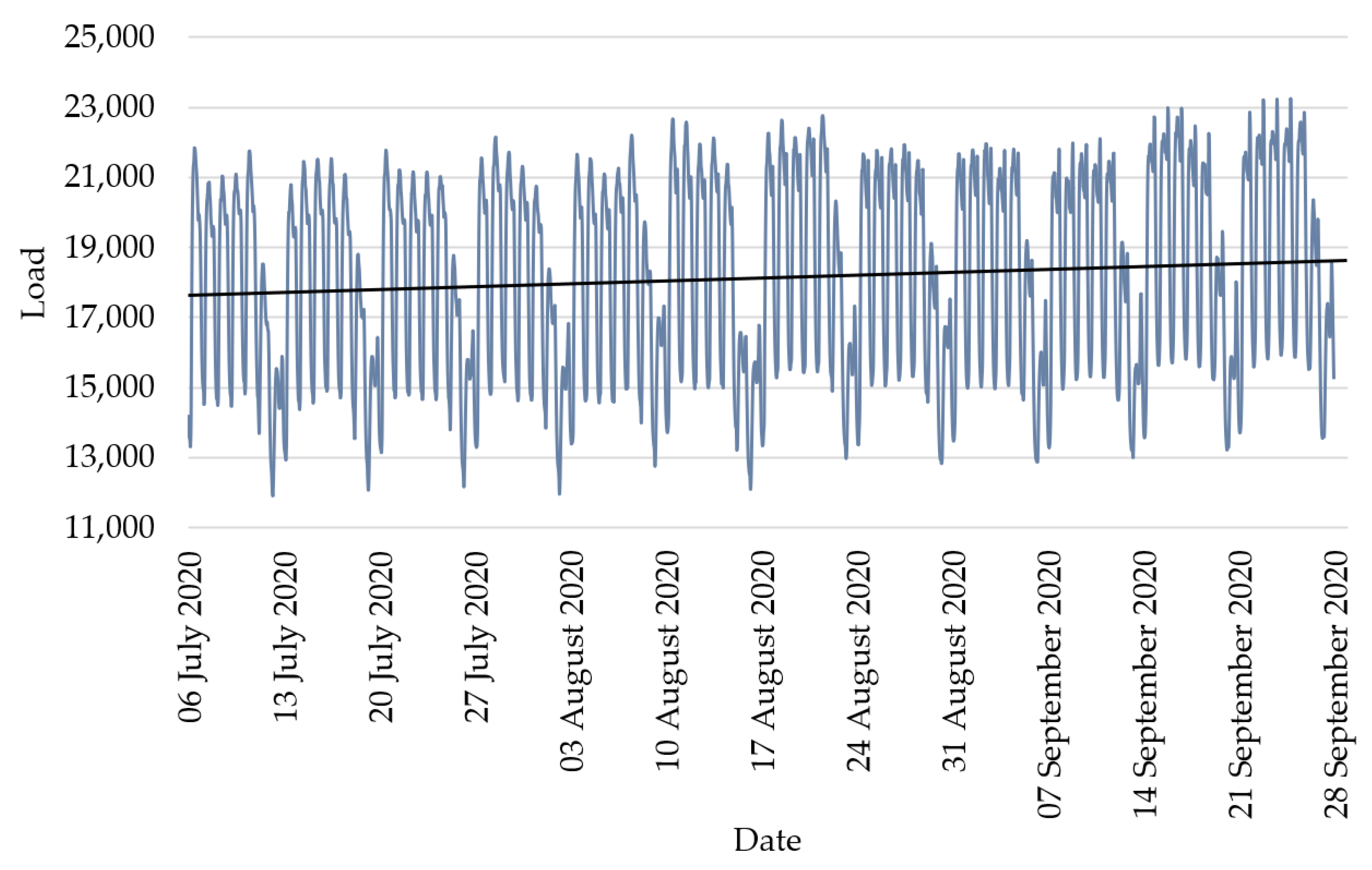
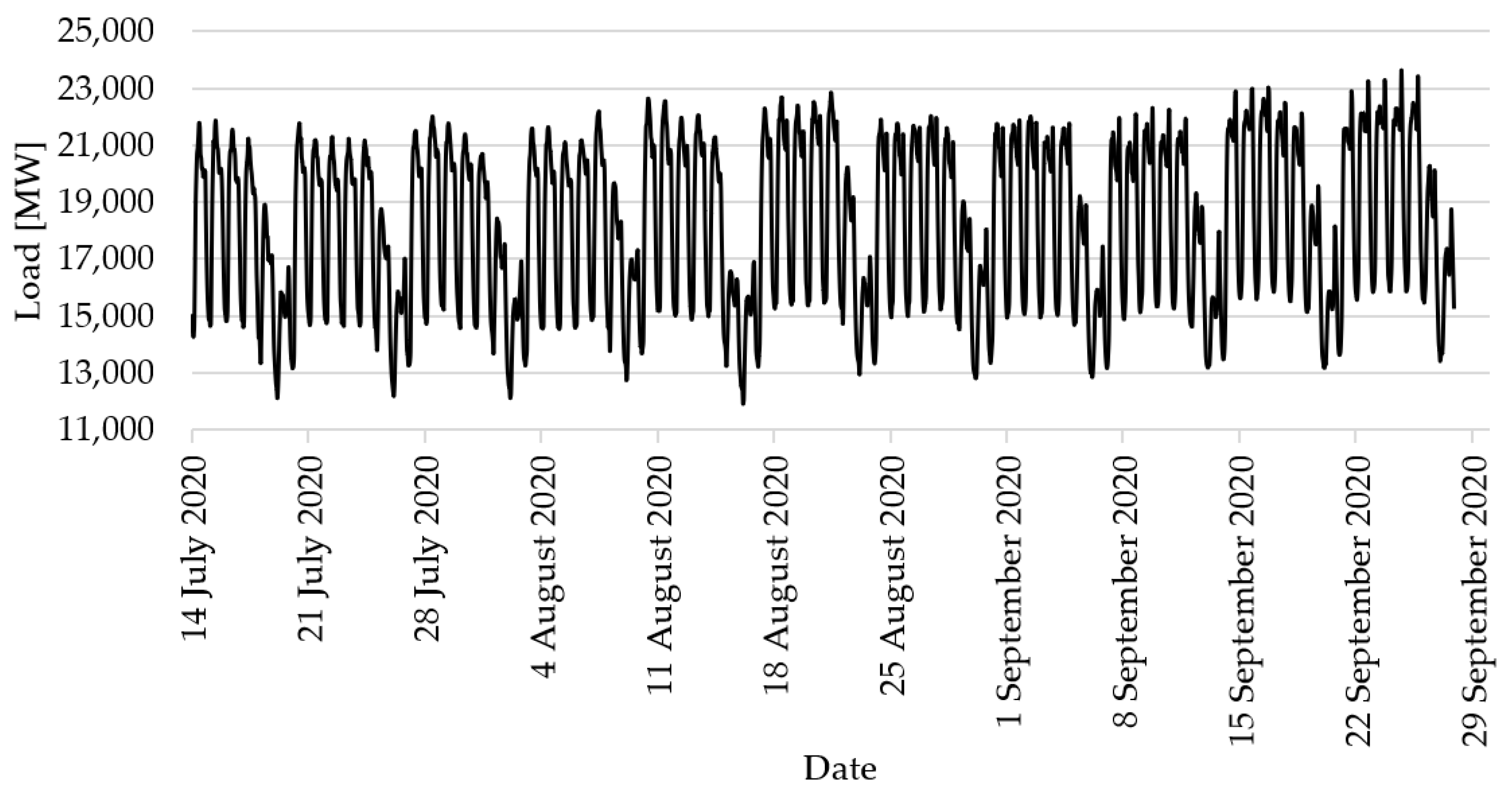
| Period of load data collection | 6 July 2020—27 September 2020 (12 weeks) |
| Number of observations | 2016 |
| Mean load | 18,134.96 MW |
| Minimum load value | 11,903.98 MW |
| Maximum load value | 23,222.25 MW |
| Load standard deviation | 2810.35 MW |
| Level of Disturbance (NSR) | Parameters | Std. Error | p-Value | 95% Confidence Interval | RMS | AIC | |
|---|---|---|---|---|---|---|---|
| Model MW | 0.20261 | 0.02382 | <0.0001 | 0.15592 | 0.24930 | 179.9524 | 21,704.73 |
| 0.72873 | 0.01860 | <0.0001 | 0.69227 | 0.76519 | |||
| 0.72605 | 0.02588 | <0.0001 | 0.67533 | 0.77677 | |||
| NSR = 10% Model + N(0; 29) | 0.21643 | 0.02368 | <0.0001 | 0.17002 | 0.26284 | 184.8383 | 21,799.42 |
| 0.72698 | 0.01863 | <0.0001 | 0.69047 | 0.76349 | |||
| 0.74025 | 0.02647 | <0.0001 | 0.68837 | 0.79213 | |||
| NSR = 20% Model + N(0; 59) | 0.28279 | 0.02307 | <0.0001 | 0.23757 | 0.32801 | 200.8707 | 22,085.67 |
| 0.74010 | 0.01829 | <0.0001 | 0.70425 | 0.77595 | |||
| 0.76365 | 0.02692 | <0.0001 | 0.71089 | 0.81641 | |||
| NSR = 30% Model + N(0; 87) | 0.35262 | 0.02239 | <0.0001 | 0.30873 | 0.39650 | 221.5301 | 22,413.83 |
| 0.76606 | 0.01763 | <0.0001 | 0.73151 | 0.80061 | |||
| 0.77243 | 0.02739 | <0.0001 | 0.71875 | 0.82611 | |||
| NSR = 50% Model + N(0; 145) | 0.46077 | 0.02104 | <0.0001 | 0.41953 | 0.50201 | 270.3925 | 23,070.28 |
| 0.78613 | 0.01738 | <0.0001 | 0.75207 | 0.82019 | |||
| 0.77771 | 0.02718 | <0.0001 | 0.72444 | 0.83098 | |||
| NSR = 100% Model + N(0; 290) | 0.68715 | 0.01615 | <0.0001 | 0.65550 | 0.71880 | 395.6171 | 24,487.19 |
| 0.83840 | 0.01525 | <0.0001 | 0.80851 | 0.86829 | |||
| 0.94662 | 0.09050 | <0.0001 | 0.76924 | 1.12400 | |||
| NSR = 200% Model + N(0; 580) | 0.84442 | 0.01165 | <0.0001 | 0.82159 | 0.86725 | 661.1075 | 26,260.64 |
| 0.89227 | 0.01441 | <0.0001 | 0.86403 | 0.92051 | |||
| 0.99989 | 45.70017 | 0.9825 | |||||
| Level of Disturbance (NSR) | Hour of 28 September 2020 | Forecast | 95% Confidence Interval | |
|---|---|---|---|---|
| From | To | |||
| NSR = 0 Model | 1 | 14,569.2799 | 14,216.5795 | 14,921.9802 |
| 2 | 14,231.1726 | 13,780.0701 | 14,682.2751 | |
| 3 | 14,074.4136 | 13,542.8222 | 14,606.0040 | |
| 4 | 14,116.8656 | 13,515.4628 | 14,718.2684 | |
| 5 | 14,552.4516 | 13,888.5380 | 15,216.3652 | |
| 6 | 15,601.6356 | 14,880.6105 | 16,322.6607 | |
| NSR = 10% Model + N(0; 29) | 1 | 14,551.6886 | 14,189.4121 | 14,913.9651 |
| 2 | 14,202.3811 | 13,742.1356 | 14,662.6266 | |
| 3 | 14,056.7153 | 13,515.9681 | 14,597.4626 | |
| 4 | 14,099.6095 | 13,488.8810 | 14,710.3380 | |
| 5 | 14,544.8341 | 13,871.3574 | 15,218.3109 | |
| 6 | 15,570.5080 | 14,839.6505 | 16,301.3655 | |
| NSR = 20% Model + N(0; 58) | 1 | 14,647.8067 | 14,254.1075 | 15,041.5060 |
| 2 | 14,239.7803 | 13,755.2924 | 14,724.2682 | |
| 3 | 14,078.4536 | 13,517.6881 | 14,639.2190 | |
| 4 | 14,183.4656 | 13,555.6223 | 14,811.3089 | |
| 5 | 14,556.4968 | 13,868.0807 | 15,244.9128 | |
| 6 | 15,640.8009 | 14,896.7270 | 16,384.8749 | |
| NSR = 30% Model + N(0;87) | 1 | 14,589.3005 | 14,155.1095 | 15,023.4915 |
| 2 | 14,265.3775 | 13,748.1437 | 14,782.6113 | |
| 3 | 14,156.0002 | 13,567.3240 | 14,744.6765 | |
| 4 | 14,189.9685 | 13,537.6275 | 14,842.3095 | |
| 5 | 14,627.1028 | 13,916.7806 | 15,337.4251 | |
| 6 | 15,659.0319 | 14,895.1165 | 16,422.9473 | |
| NSR = 50% Model + N(0; 145) | 1 | 14,334.9439 | 13,804.9843 | 14,864.9036 |
| 2 | 13,984.5530 | 13,382.4542 | 14,586.6518 | |
| 3 | 13,749.7201 | 13,083.2452 | 14,416.1949 | |
| 4 | 13,784.8641 | 13,059.7058 | 14,510.0223 | |
| 5 | 14,203.5181 | 13,424.0823 | 14,982.9539 | |
| 6 | 15,435.2713 | 14,605.0991 | 16,265.4435 | |
| NSR = 100% Model + N(0; 290) | 1 | 14,146.3251 | 13,370.9299 | 14,921.7203 |
| 2 | 14,264.9867 | 13,452.5307 | 15,077.4426 | |
| 3 | 14,028.2346 | 13,180.3362 | 14,876.1329 | |
| 4 | 14,113.0099 | 13,231.0924 | 14,994.9275 | |
| 5 | 14,410.1252 | 13,495.4529 | 15,324.7976 | |
| 6 | 15,543.8580 | 14,597.5639 | 16,490.1521 | |
| NSR = 200% Model + N(0; 580) | 1 | 14,379.1325 | 13,083.3855 | 15,674.8794 |
| 2 | 14,358.8916 | 13,047.5563 | 15,670.2269 | |
| 3 | 14,624.8744 | 13,298.1340 | 15,951.6149 | |
| 4 | 14,357.8940 | 13,015.9252 | 15,699.8628 | |
| 5 | 14,853.3425 | 13,496.3162 | 16,210.3688 | |
| 6 | 15,746.6589 | 14,374.7404 | 17,118.5774 | |
Publisher’s Note: MDPI stays neutral with regard to jurisdictional claims in published maps and institutional affiliations. |
© 2021 by the authors. Licensee MDPI, Basel, Switzerland. This article is an open access article distributed under the terms and conditions of the Creative Commons Attribution (CC BY) license (https://creativecommons.org/licenses/by/4.0/).
Share and Cite
Chodakowska, E.; Nazarko, J.; Nazarko, Ł. ARIMA Models in Electrical Load Forecasting and Their Robustness to Noise. Energies 2021, 14, 7952. https://doi.org/10.3390/en14237952
Chodakowska E, Nazarko J, Nazarko Ł. ARIMA Models in Electrical Load Forecasting and Their Robustness to Noise. Energies. 2021; 14(23):7952. https://doi.org/10.3390/en14237952
Chicago/Turabian StyleChodakowska, Ewa, Joanicjusz Nazarko, and Łukasz Nazarko. 2021. "ARIMA Models in Electrical Load Forecasting and Their Robustness to Noise" Energies 14, no. 23: 7952. https://doi.org/10.3390/en14237952
APA StyleChodakowska, E., Nazarko, J., & Nazarko, Ł. (2021). ARIMA Models in Electrical Load Forecasting and Their Robustness to Noise. Energies, 14(23), 7952. https://doi.org/10.3390/en14237952