
Water Hammer Control Using Additional Branched HDPE Pipe

 ,
,  ,
,  , and
, and 
Abstract
:1. Introduction
2. Hydraulic Transient Model
3. Experimental Study
4. Analysis of Experimental Data
5. Numerical Solution and Model Validation
6. Conclusions
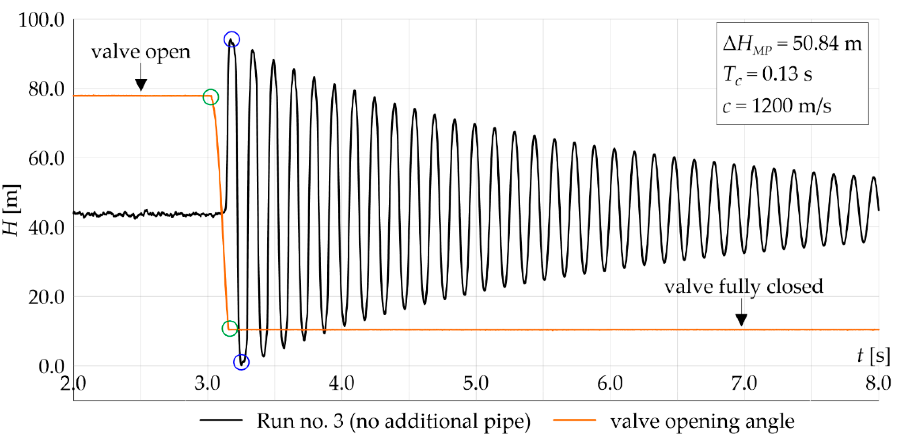
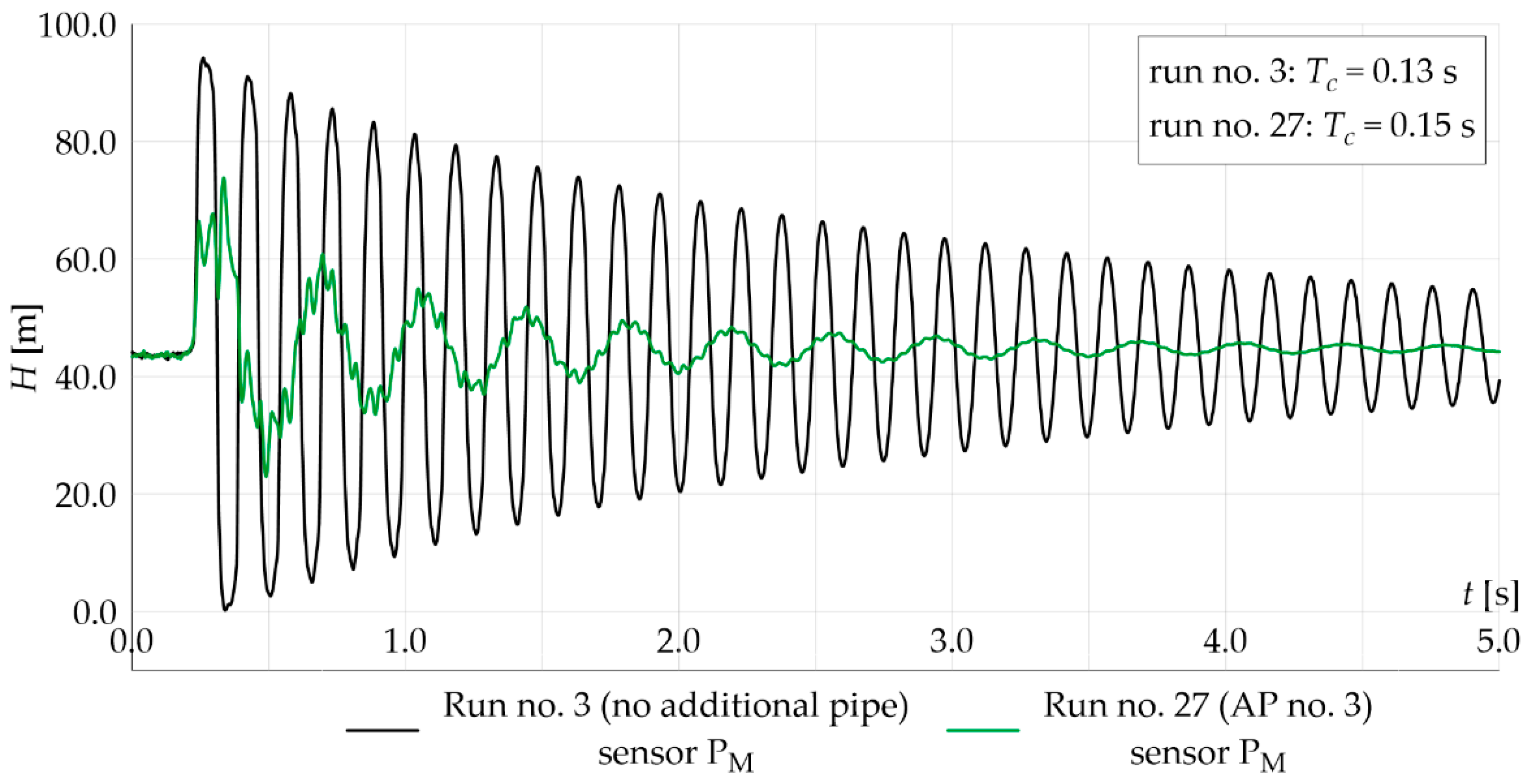
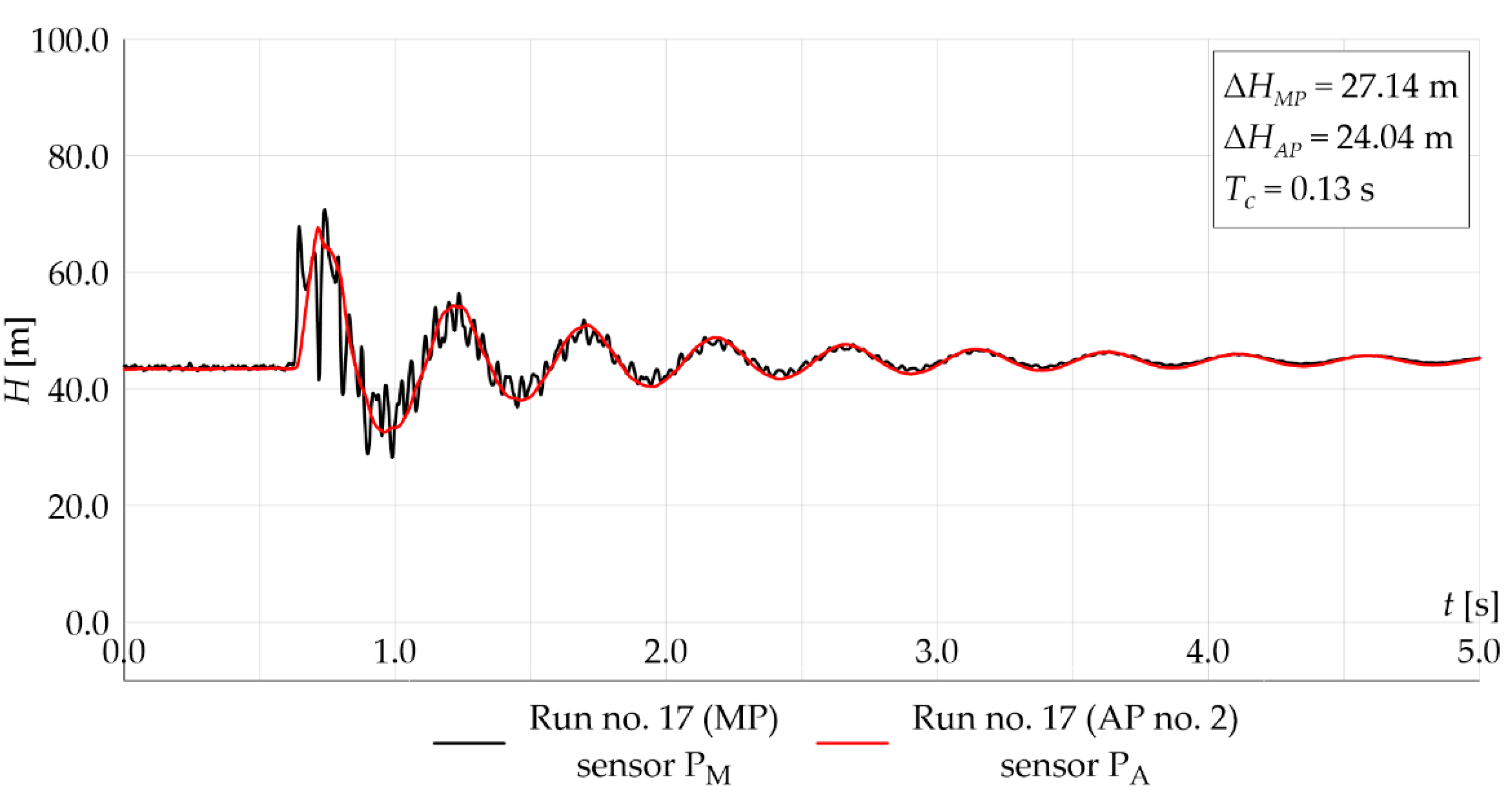
- The experimental tests showed that the additional polymeric pipe can be successfully used to attenuate a pressure surge during a water hammer event induced by rapid valve closure. Comparing the pressure oscillations in the pipeline with and without the device, it is apparent that an additional pipe significantly reduces the maximum pressure increase and reduces the duration of the phenomenon.
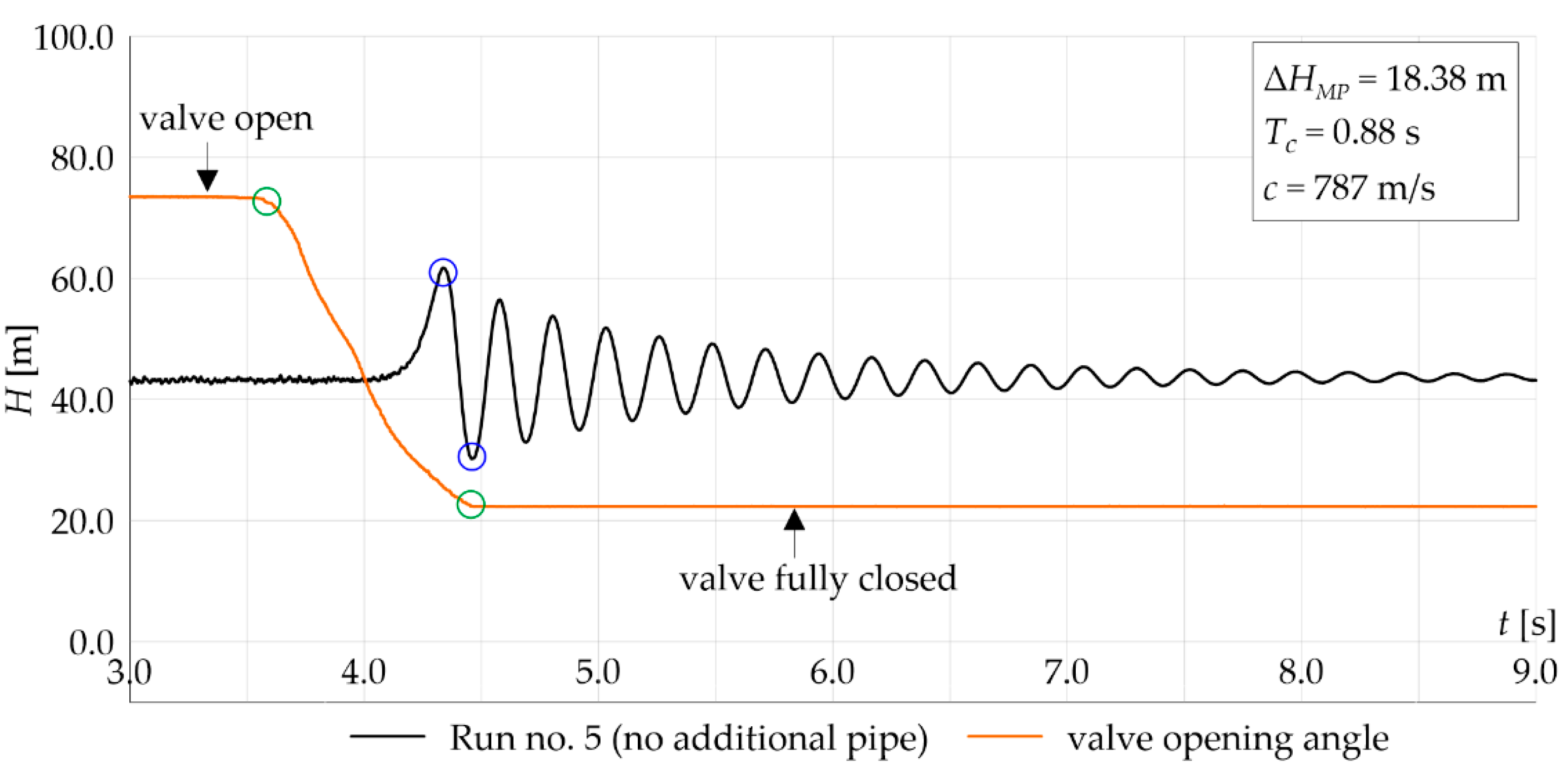
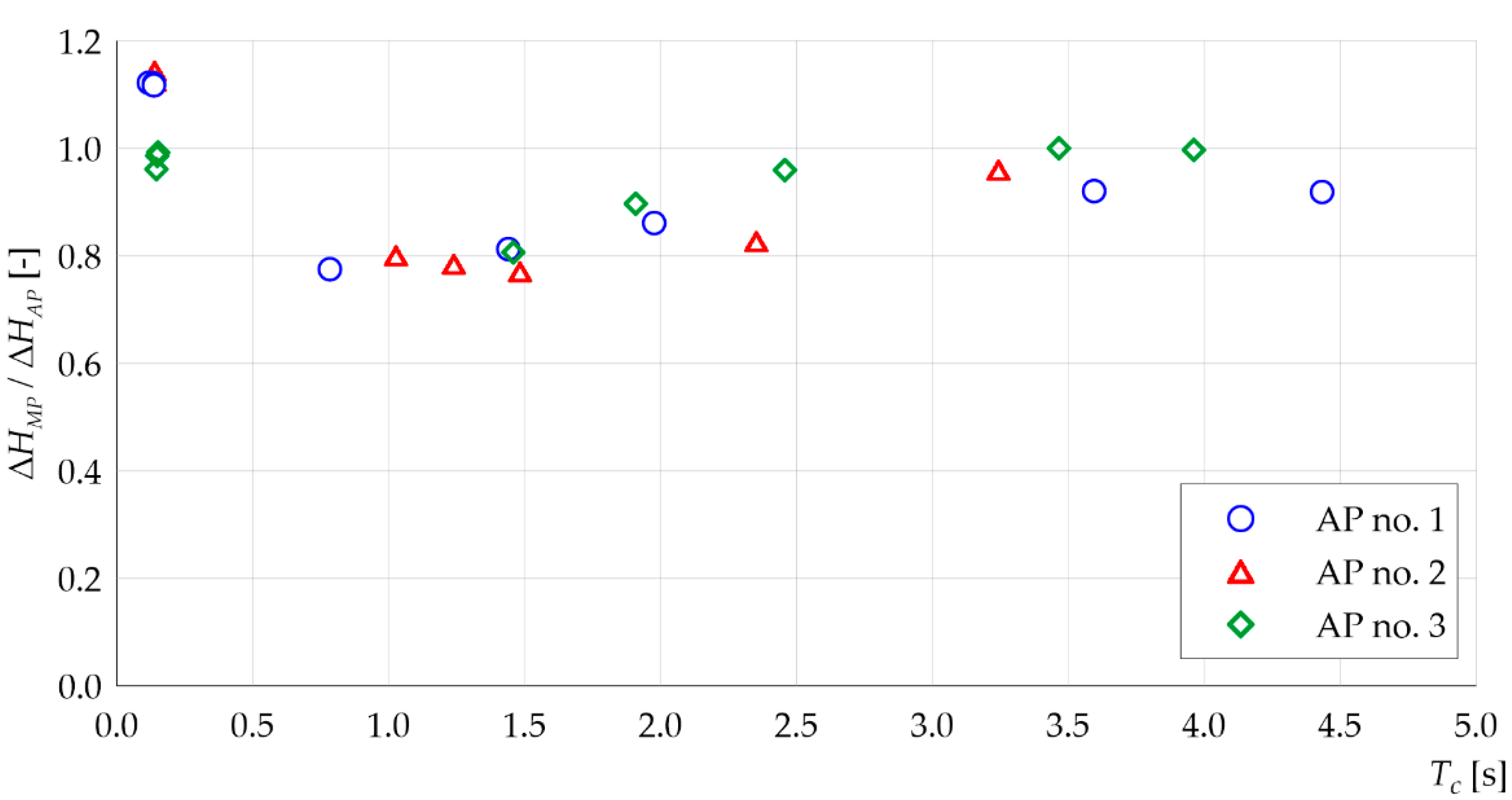
- As the valve closing time lengthens, the influence of the additional pipe on the maximum pressure increase is reduced. Results of experimental runs showed that, during less severe hydraulic transients, values of maximum pressure increase in the pipeline, with and without the device, are similar. Thus, additional HDPE pipe does not provide notable protection against hydraulic transients induced by slow valve closure in terms of reducing the first pressure peak.
- In all analysed cases, both for rapid and slow valve closures, the presence of a polymeric additional pipe causes a reduction in pressure wave velocity and lengthens the period of pressure oscillations.
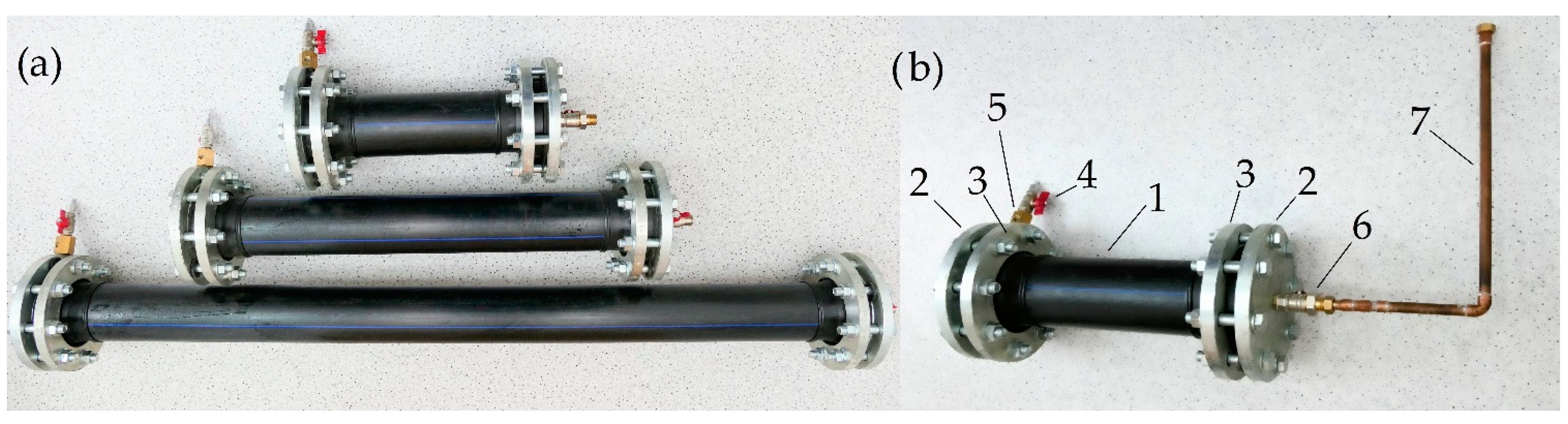
- In this study, the performance of three devices with different volumes was experimentally analysed. The apparent lack of correlation between the volume of the additional polymeric pipe and its ability to attenuate pressure waves can be attributed to the small diameter of the connection pipe compared with the diameter of the device. This way of connecting additional pipes to the main pipeline, although justified by practical reasons, makes the device less effective. Further data collection is required to evaluate the influence of the connection pipe on the performance of the additional polymeric pipes.
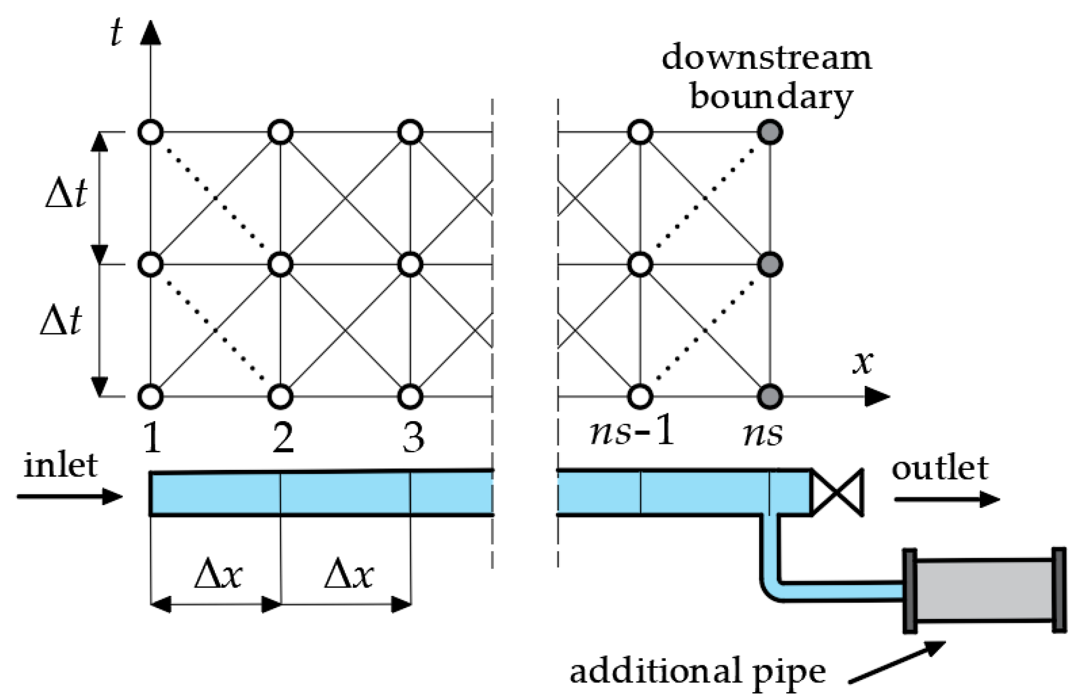
- In order to simulate the water hammer phenomenon, a numerical model in which an additional pipe is treated as a lumped parameter was used. Experimental data was used to calibrate the mechanical properties of the pipeline system. The calculation results showed that this approach allows the reasonable reproduction of unsteady flow oscillations registered during experiments, in terms of maximum pressure increase and pressure wave oscillation period.
Author Contributions
Funding
Institutional Review Board Statement
Informed Consent Statement
Data Availability Statement
Conflicts of Interest
Nomenclature
| A | cross sectional area of the main pipeline (m2) |
| c | pressure wave velocity in the main pipeline (m/s) |
| cAP | pressure wave velocity in the additional pipe (m/s) |
| D | main pipeline internal diameter (m) |
| DAP | additional pipe internal diameter (m) |
| DAP0 | inner diameter of the additional pipe at time t = 0 |
| f | friction factor (-) |
| g | gravity acceleration (m/s2) |
| i | number of a single Kelvin–Voigt element (-) |
| H | piezometric head (m) |
| J(t) | creep compliance at time t (Pa−1) |
| J(t’) | creep compliance at time t’ (Pa−1) |
| LAP | length of the additional pipe (m) |
| n | total number of Kelvin–Voigt elements (-) |
| Q | volumetric flow rate (m3/s) |
| p0 | initial pressure (Pa) |
| p(t) | pressure at time t (Pa) |
| SAP | additional pipe wall thickness (m) |
| TC | valve closing time (s) |
| t | time (s) |
| v0 | initial average flow velocity (m/s) |
| vi,L | velocity on the left hand side of the connection node (m/s) |
| vi,R | velocity on the right hand side of the connection node (m/s) |
| WAP | volume of the additional pipe (m3) |
| WMP | volume of the main pipeline (m3) |
| x | space coordinate (m) |
| ΔHAP | maximum pressure increase in the additional pipe (Pa) |
| ΔHMP | maximum pressure increase in the main pipeline (Pa) |
| Δt | time step (s) |
| Δx | spatial step (m) |
| ε | unit instantaneous strain (-) |
| ε0 | instantaneous (elastic) strain (-) |
| εr | retarded strain (-) |
| σ | stress (Pa) |
| τi | the retardation time of i-th Kelvin–Voigt element (s) |
| Acronyms | |
| AP | additional pipe |
| DAQ | data acquisition system |
| MOC | method of characteristics |
| HDPE | high-density polyethylene |
| MP | main pipeline |
References
- Bergant, A.; Simpson, A.R.; Tijsseling, A.S. Water hammer with column separation: A historical review. J. Fluids Struct. 2006, 22, 135–171. [Google Scholar] [CrossRef] [Green Version]
- Ramos, H.; Covas, D.; Borga, A.; Loureiro, D. Surge damping analysis in pipe systems: Modelling and experiments. J. Hydraul. Res. 2004, 42, 413–425. [Google Scholar] [CrossRef]
- Bazargan-Lari, M.R.; Kerachian, R.; Afshar, H.; Bashi-Azghadi, S.N. Developing an optimal valve closing rule curve for real-time pressure control in pipes. J. Mech. Sci. Technol. 2013, 27, 215–225. [Google Scholar] [CrossRef]
- Wan, W.; Li, F. Sensitivity Analysis of Operational Time Differences for a Pump–Valve System on a Water Hammer Response. J. Press. Vessel. Technol. 2016, 138, 011303. [Google Scholar] [CrossRef]
- Yu, X.; Zhang, J.; Miao, D. Innovative Closure Law for Pump-Turbines and Field Test Verification. J. Hydraul. Eng. 2015, 141, 05014010. [Google Scholar] [CrossRef]
- Zhou, J.; Xu, Y.; Zheng, Y.; Zhang, Y. Optimization of Guide Vane Closing Schemes of Pumped Storage Hydro Unit Using an Enhanced Multi-Objective Gravitational Search Algorithm. Energies 2017, 10, 911. [Google Scholar] [CrossRef]
- Pérez-Sánchez, M.; López-Jiménez, P.; Ramos, H. PATs Operating in Water Networks under Unsteady Flow Conditions: Control Valve Manoeuvre and Overspeed Effect. Water 2018, 10, 529. [Google Scholar] [CrossRef] [Green Version]
- Subani, N.; Amin, N. Analysis of Water Hammer with Different Closing Valve Laws on Transient Flow of Hydrogen-Natural Gas Mixture. Abstr. Appl. Anal. 2015, 2015, 510675. [Google Scholar] [CrossRef] [Green Version]
- Boulos, P.F.; Karney, B.W.; Wood, D.J.; Lingireddy, S. Hydraulic Transient Guidelines for Protecting Water Distribution Systems. J. Am. Water Work. Assoc. 2005, 97, 111–124. [Google Scholar] [CrossRef]
- Chaudhry, M.H. Applied Hydraulic Transients, 3rd ed.; Springer: New York, NY, USA, 2014; ISBN 978-1-4614-8538-4. [Google Scholar]
- Stephenson, D. Simple Guide for Design of Air Vessels for Water Hammer Protection of Pumping Lines. J. Hydraul. Eng. 2002, 128, 792–797. [Google Scholar] [CrossRef]
- Kim, S.-G.; Lee, K.-B.; Kim, K.-Y. Water hammer in the pump-rising pipeline system with an air chamber. J. Hydrodyn. 2014, 26, 960–964. [Google Scholar] [CrossRef]
- Wan, W.; Zhang, B.; Chen, X.; Lian, J. Water Hammer Control Analysis of an Intelligent Surge Tank with Spring Self-Adaptive Auxiliary Control System. Energies 2019, 12, 2527. [Google Scholar] [CrossRef] [Green Version]
- Wan, W.; Zhang, B. Investigation of Water Hammer Protection in Water Supply Pipeline Systems Using an Intelligent Self-Controlled Surge Tank. Energies 2018, 11, 1450. [Google Scholar] [CrossRef] [Green Version]
- Riasi, A.; Nourbakhsh, A. Influence of Surge Tank and Relief Valve on Transient Flow Behaviour in Hydropower Stations. In Proceedings of the ASME-JSME-KSME 2011 Joint Fluids Engineering Conference, Hamamatsu, Japan, 24–29 July 2011; Symposia–Parts A, B, C, and D.; ASMEDC: Hamamatsu, Japan, 2011; Volume 1, pp. 1971–1977. [Google Scholar]
- Vereide, K.; Svingen, B.; Nielsen, T.K.; Lia, L. The Effect of Surge Tank Throttling on Governor Stability, Power Control, and Hydraulic Transients in Hydropower Plants. IEEE Trans. Energy Convers. 2017, 32, 91–98. [Google Scholar] [CrossRef] [Green Version]
- Balacco, G.; Apollonio, C.; Piccinni, A.F. Experimental analysis of air valve behaviour during hydraulic transients. J. Appl. Water Eng. Res. 2015, 3, 3–11. [Google Scholar] [CrossRef]
- Zhang, K.Q.; Karney, B.W.; McPherson, D.L. Pressure-relief valve selection and transient pressure control. J. Am. Water Work. Assoc. 2008, 100, 62–69. [Google Scholar] [CrossRef]
- Kim, H.; Kim, S. Optimization of pressure relief valve for pipeline system under transient induced cavitation condition. Urban Water J. 2019, 16, 718–726. [Google Scholar] [CrossRef]
- Bettaieb, N.; Taieb, E.H. Assessment of Failure Modes Caused by Water Hammer and Investigation of Convenient Control Measures. J. Pipeline Syst. Eng. Pract. 2020, 11, 04020006. [Google Scholar] [CrossRef]
- Mery, H.O.; Hassan, J.M.; EKaid, A.L. Water Hammer Mitigation by Air Vessel and Bypass Forward Configuration. IOP Conf. Ser. Mater. Sci. Eng. 2021, 1094, 012052. [Google Scholar] [CrossRef]
- Wróbel, J.; Blaut, J. Influence of Pressure inside a Hydraulic Line on Its Natural Frequencies and Mode Shapes. In Advances in Hydraulic and Pneumatic Drives and Control 2020; Stryczek, J., Warzyńska, U., Eds.; Lecture Notes in Mechanical Engineering; Springer International Publishing: Cham, Switzerland, 2021; pp. 333–343. ISBN 978-3-030-59508-1. [Google Scholar]
- Kubrak, M.; Kodura, A. Water Hammer Phenomenon in Pipeline with Inserted Flexible Tube. J. Hydraul. Eng. 2020, 146, 04019054. [Google Scholar] [CrossRef]
- Pezzinga, G.; Scandura, P. Unsteady Flow in Installations with Polymeric Additional Pipe. J. Hydraul. Eng. 1995, 121, 802–811. [Google Scholar] [CrossRef]
- Pezzinga, G. Unsteady Flow in Hydraulic Networks with Polymeric Additional Pipe. J. Hydraul. Eng. 2002, 128, 238–244. [Google Scholar] [CrossRef]
- Triki, A. Water-hammer control in pressurized-pipe flow using an in-line polymeric short-section. Acta Mech. 2016, 227, 777–793. [Google Scholar] [CrossRef]
- Triki, A. Comparative assessment of the inline and branching design strategies based on the compound technique. J. Water Supply Res. Technol.–Aqua 2021, 70, 155–170. [Google Scholar] [CrossRef]
- Triki, A. Water-Hammer Control in Pressurized-Pipe Flow Using a Branched Polymeric Penstock. J. Pipeline Syst. Eng. Pract. 2017, 8, 04017024. [Google Scholar] [CrossRef]
- Triki, A.; Trabelsi, M. On the in-series and branching dual-technique–based water-hammer control strategy. Urban Water J. 2021, 18, 631–639. [Google Scholar] [CrossRef]
- Covas, D.; Stoianov, I.; Mano, J.F.; Ramos, H.; Graham, N.; Maksimovic, C. The dynamic effect of pipe-wall viscoelasticity in hydraulic transients. Part II—model development, calibration and verification. J. Hydraul. Res. 2005, 43, 56–70. [Google Scholar] [CrossRef]
- Keramat, A.; Tijsseling, A.S.; Hou, Q.; Ahmadi, A. Fluid–structure interaction with pipe-wall viscoelasticity during water hammer. J. Fluids Struct. 2012, 28, 434–455. [Google Scholar] [CrossRef] [Green Version]
- Keramat, A.; Kolahi, A.G.; Ahmadi, A. Waterhammer modelling of viscoelastic pipes with a time-dependent Poisson’s ratio. J. Fluids Struct. 2013, 43, 164–178. [Google Scholar] [CrossRef]
- Kodura, A. An Analysis of the Impact of Valve Closure Time on the Course of Water Hammer. Arch. Hydro-Eng. Environ. Mech. 2016, 63, 35–45. [Google Scholar] [CrossRef] [Green Version]
- Malesinska, A.; Kubrak, M.; Rogulski, M.; Puntorieri, P.; Fiamma, V.; Barbaro, G. Water Hammer Simulation in a Steel Pipeline System with a Sudden Cross-section Change. J. Fluids Eng. 2021, 143, 091204. [Google Scholar] [CrossRef]
- Brunone, B.; Meniconi, S.; Capponi, C. Numerical analysis of the transient pressure damping in a single polymeric pipe with a leak. Urban Water J. 2018, 15, 760–768. [Google Scholar] [CrossRef]
- Bergant, A.; Tijsseling, A.S.; Vítkovský, J.P.; Covas, D.I.C.; Simpson, A.R.; Lambert, M.F. Parameters affecting water-hammer wave attenuation, shape and timing—Part 1: Mathematical tools. J. Hydraul. Res. 2008, 46, 373–381. [Google Scholar] [CrossRef] [Green Version]
- Evangelista, S.; Leopardi, A.; Pignatelli, R.; de Marinis, G. Hydraulic Transients in Viscoelastic Branched Pipelines. J. Hydraul. Eng. 2015, 141, 04015016. [Google Scholar] [CrossRef]
- Duan, H.-F.; Ghidaoui, M.; Lee, P.J.; Tung, Y.-K. Unsteady friction and visco-elasticity in pipe fluid transients. J. Hydraul. Res. 2010, 48, 354–362. [Google Scholar] [CrossRef]
- Pal, S.; Hanmaiahgari, P.R.; Karney, B.W. An Overview of the Numerical Approaches to Water Hammer Modelling: The Ongoing Quest for Practical and Accurate Numerical Approaches. Water 2021, 13, 1597. [Google Scholar] [CrossRef]
- Bertaglia, G.; Ioriatti, M.; Valiani, A.; Dumbser, M.; Caleffi, V. Numerical methods for hydraulic transients in visco-elastic pipes. J. Fluids Struct. 2018, 81, 230–254. [Google Scholar] [CrossRef] [Green Version]
- Bogdevičius, M.; Karpenko, M.; Bogdevičius, P. Determination of rheological model coefficients of pipeline composite material layers based on spectrum analysis and optimization. J. Theor. Appl. Mech. 2021, 265–278. [Google Scholar] [CrossRef]
- Weinerowska-Bords, K. Viscoelastic Model of Waterhammer in Single Pipeline–Problems and Questions. Arch. Hydro-Eng. Environ. Mech. 2006, 53, 21. [Google Scholar]
- Weinerowska-Bords, K. Alternative Approach to Convolution Term of Viscoelasticity in Equations of Unsteady Pipe Flow. J. Fluids Eng. 2015, 137, 054501. [Google Scholar] [CrossRef]


| AP Number | LAP [m] | DAP [m] | SAP [m] | WAP [m3] | WAP/WMP [–] |
|---|---|---|---|---|---|
| 1 | 0.40 | 0.086 | 0.012 | 0.0023 | 0.02 |
| 2 | 0.80 | 0.086 | 0.012 | 0.0046 | 0.04 |
| 3 | 1.50 | 0.086 | 0.012 | 0.0087 | 0.08 |
| Run | Variant of Experiment | Type of Valve Closure | v0 [m/s] | TC [s] | ΔHMP [MPa] | ΔHAP [MPa] | c [m/s] |
|---|---|---|---|---|---|---|---|
| 1 | no AP | rapid | 0.38 | 0.14 | 49.79 | - | 1143 |
| 2 | no AP | rapid | 0.39 | 0.14 | 50.33 | - | 1171 |
| 3 | no AP | rapid | 0.39 | 0.13 | 50.84 | - | 1200 |
| 4 | no AP | slow | 0.40 | 0.77 | 24.68 | - | 828 |
| 5 | no AP | slow | 0.39 | 0.88 | 18.38 | - | 787 |
| 6 | no AP | slow | 0.41 | 1.53 | 15.89 | - | 727 |
| 7 | no AP | slow | 0.39 | 2.99 | 10.29 | - | 701 |
| 8 | no AP | slow | 0.40 | 4.87 | 4.85 | - | 238 |
| 9 | AP no. 1 | rapid | 0.38 | 0.12 | 29.83 | 26.58 | 407 |
| 10 | AP no. 1 | rapid | 0.38 | 0.14 | 29.29 | 26.16 | 407 |
| 11 | AP no. 1 | rapid | 0.39 | 0.14 | 29.74 | 26.63 | 407 |
| 12 | AP no. 1 | slow | 0.38 | 0.78 | 17.91 | 23.10 | 425 |
| 13 | AP no. 1 | slow | 0.39 | 1.44 | 14.26 | 17.55 | 417 |
| 14 | AP no. 1 | slow | 0.39 | 1.98 | 13.07 | 15.18 | 407 |
| 15 | AP no. 1 | slow | 0.39 | 3.59 | 8.65 | 9.39 | 358 |
| 16 | AP no. 1 | slow | 0.38 | 4.43 | 9.18 | 9.99 | 381 |
| 17 | AP no. 2 | rapid | 0.39 | 0.13 | 27.14 | 24.04 | 393 |
| 18 | AP no. 2 | rapid | 0.39 | 0.14 | 27.18 | 24.17 | 397 |
| 19 | AP no. 2 | rapid | 0.39 | 0.14 | 26.80 | 23.44 | 393 |
| 20 | AP no. 2 | slow | 0.39 | 1.03 | 17.43 | 21.71 | 410 |
| 21 | AP no. 2 | slow | 0.39 | 1.24 | 16.76 | 21.35 | 403 |
| 22 | AP no. 2 | slow | 0.39 | 1.48 | 14.78 | 19.17 | 400 |
| 23 | AP no. 2 | slow | 0.38 | 2.35 | 13.84 | 16.74 | 414 |
| 24 | AP no. 2 | slow | 0.38 | 3.24 | 7.15 | 7.45 | 333 |
| 25 | AP no. 3 | rapid | 0.38 | 0.15 | 31.22 | 31.66 | 480 |
| 26 | AP no. 3 | rapid | 0.39 | 0.15 | 30.30 | 31.51 | 480 |
| 27 | AP no. 3 | rapid | 0.39 | 0.15 | 30.87 | 31.11 | 480 |
| 28 | AP no. 3 | slow | 0.38 | 1.46 | 17.74 | 21.99 | 533 |
| 29 | AP no. 3 | slow | 0.38 | 1.91 | 13.20 | 14.71 | 505 |
| 30 | AP no. 3 | slow | 0.38 | 2.46 | 8.73 | 9.10 | 421 |
| 31 | AP no. 3 | slow | 0.39 | 3.46 | 6.32 | 6.32 | 378 |
| 32 | AP no. 3 | slow | 0.39 | 3.96 | 6.11 | 6.13 | 385 |
Publisher’s Note: MDPI stays neutral with regard to jurisdictional claims in published maps and institutional affiliations. |
© 2021 by the authors. Licensee MDPI, Basel, Switzerland. This article is an open access article distributed under the terms and conditions of the Creative Commons Attribution (CC BY) license (https://creativecommons.org/licenses/by/4.0/).
Share and Cite
Kubrak, M.; Malesińska, A.; Kodura, A.; Urbanowicz, K.; Bury, P.; Stosiak, M. Water Hammer Control Using Additional Branched HDPE Pipe. Energies 2021, 14, 8008. https://doi.org/10.3390/en14238008
Kubrak M, Malesińska A, Kodura A, Urbanowicz K, Bury P, Stosiak M. Water Hammer Control Using Additional Branched HDPE Pipe. Energies. 2021; 14(23):8008. https://doi.org/10.3390/en14238008
Chicago/Turabian StyleKubrak, Michał, Agnieszka Malesińska, Apoloniusz Kodura, Kamil Urbanowicz, Paweł Bury, and Michał Stosiak. 2021. "Water Hammer Control Using Additional Branched HDPE Pipe" Energies 14, no. 23: 8008. https://doi.org/10.3390/en14238008
APA StyleKubrak, M., Malesińska, A., Kodura, A., Urbanowicz, K., Bury, P., & Stosiak, M. (2021). Water Hammer Control Using Additional Branched HDPE Pipe. Energies, 14(23), 8008. https://doi.org/10.3390/en14238008