Abstract
To help stakeholders plan, research, and develop Hybrid Renewable Energy Systems (HRES), the elaboration of numerous modelling techniques and software simulation tools has been reported. The thorough analysis of these undoubtedly complex systems is strongly correlated with the efficient utilisation of the potential of renewable energy and the meticulous development of pertinent designs. In this context, various optimisation constraints/targets have also been utilised. This specific work initially carries out a thorough review of the modelling techniques and simulation software developed in an attempt to define a commonly accepted categorisation methodology for the various existing HRES simulation methods. Moreover, the widely utilised optimisation targets are analysed in detail. Finally, it identifies the sensitivity of two commercial software tools (HOMER Pro and iHOGA) by examining nine case studies based on different wind and solar potential combinations. The results obtained by the two commercial tools are compared with the ESA Microgrid Simulator, a software developed by the Soft Energy Applications and Environmental Protection Laboratory of the Mechanical Engineering Department of the University of West Attica. The evaluation of the results, based on the diversification of the renewable energy potential used as input, has led to an in-depth assessment of the deviances detected in the software tools selected.
1. Introduction
The imminent depletion of fossil fuel reserves and the continuous increase in energy demand have urged the need for renewable energy sources, such as wind and solar energy, to fulfil the electricity needs in urban or remote areas [1]. Indisputably, the ubiquitous, environmentally friendly and inexhaustible features of renewable energy sources are counterbalanced by their intermittent/stochastic nature. Moreover, the possible mismatch between the profiles of the energy generation and the load demand prerequisites the integration of energy storage technologies into the energy systems configurations in order to attain the best possible exploitation of renewable energy potential prevailing in a specific region [2,3]. Albeit the significant scientific leaps noted in the development of the aforementioned technologies in the previous years, they are still considered remarkably capital intensive, enhancing the requirement for extensive and continuous research in that field in order to attain economies of scale [4].
Hybrid Renewable Energy Systems (HRES) are considered one of the most promising and trustworthy alternatives to the main electricity grid for the electrification of remote consumers, as they contribute to mitigating climate change and minimising the use of fossil fuels [5]. HRES’ main assets in comparison to single energy source-based systems are [4,6]:
- High reliability;
- Minimisation of energy storage capacity requirement, especially if the hybrid energy system is comprised of RES with a complementary character as solar and wind energy are;
- Better efficiency;
- Modularity;
- LCOE (Levelised Cost Of Electricity) minimisation (as a consequence of an optimum design strategy).
A defectively designed and unorganised development of HRES projects can lead to an elevated implied investment cost. Thus, numerous modelling techniques, as well as simulation software, have been deployed to serve as assets to HRES stakeholders’ research, planning, and development scopes [7]. HRES simulation in fact includes solving numerical formulas that outline the mathematical models for the function of the pertinent HRES components. In this way, the system behaviour can be enlightened and the project decision-making process supported [8]. It is worth noting that the simulation methods generate non-identical combinations of renewable energy systems according to the input parameters selected/imported by the user (e.g., meteorological data, size parameters range, etc.) [9,10]. The non-identical combinations proposed by the various simulation methods are basically ascribed to their intrinsic diversified dispatch strategy [11].
The HRES performance optimisation shall be based on a reliable technique, given the system’s components characteristics, the area terrain, and the meteorological data. Figure 1 depicts an overview of the parameters that consist a pertinent HRES optimisation process. Despite being considered a complex task, efficient understanding, analysis, design, and planning of a HRES project necessitates to conduct an extensive theoretical prefeasibility analysis and explore in detail the validity of its results through specialised simulation software and pertinent scenarios adopted as case studies [4,9]. Thus, the thorough HRES analysis is strongly correlated with the efficient utilisation of RES potential and the projects’ meticulous design [12]. In this context, a well-designed and optimal sizing process can be considered as the “holy grail” for the HRES optimised functionality [13].
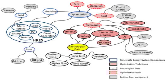
Figure 1.
Overview of HRES optimisation process [6].
An “ideal” simulation method capable of integrating all aspects of the penetration of renewable energy into hybrid energy systems does not exist [14,15,16]. The complexity of a perfect HRES modelling process implies a great simulation burden. Thus, to create a satisfactory model one must balance both accuracy and complexity [6]. The maturity of optimisation models with a general resonance in the scientific community has not yet reached the desired level, representing a path in need of further clarification and research. Various tools have been developed in this context. Multi-criteria decision analysis based on the results of a great number of simulation techniques is the most widely adopted among them, serving best engineering practices and future optimisation scopes [17].
Most scientific studies concerning HRES (consisting principally of solar and wind power) are mainly evaluated with economic factors and on a second level with power reliability indicators (Figure 2). Thus, the last ones, along with environmental indicators (especially when conventional electricity-generating resources are included in the HRES), shall be further analysed.
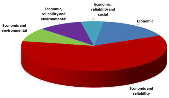
Figure 2.
Allocation of assessment parameters adopted for appraisal of standalone HRES (with solar and wind power being its main ingredients) since 2012 (adapted from [10]).
The vast majority of scientific papers issued utilise two commercial software to conduct the relevant simulations, namely HOMER (Hybrid Optimisation of Multiple Energy Resources) and iHOGA (improved Hybrid Optimisation by Genetic Algorithms), which are developed by NREL (National Renewable Energy Laboratory) and the University of Zaragoza, respectively [18,19]. In this respect, the specific work identifies the sensitivity of these commercial software by examining nine case studies under the prism of covering the electricity needs of a remote domestic consumer, based on different combinations of solar and wind potential. The results are collated with the ESA Microgrid Simulator, developed by the Soft Energy Applications and Environmental Protection Laboratory (SEALAB) of the Mechanical Engineering Department of the University of West Attica in the framework of a relevant innovation project [20]. The ESA examines different hybrid energy systems configurations, aiming at their optimisation with multi-criteria analysis. Additionally, ESA has the ability to implement DSM (Demand Side Management) techniques and the capability of handling the presence of electric vehicles inside the various energy systems’ configurations, aiming at optimum exploitation of RES generation. A detailed assessment of the discrepancies between the selected software tools has been obtained by the evaluation of the results, depending on the diversification of the renewable energy potential used as input.
2. Optimisation Techniques Review
Concerning the HRES optimal sizing, Subramanian et al. classified the energy systems modelling techniques in two categories based on the criteria of the modelling approach and the application field [8]. Following another approach, Ghofrani and Hosseini [21] classified the main optimisation algorithms into three categories: the classical algorithms, the metaheuristic algorithms and the hybrid combination of the aforementioned categories. In their turn, Tina et al. [22] and also Khatod et al. [23] classified the energy systems’ modelling techniques in analytical and simulation or MCS (Monte Carlo Simulations) methods. The last category was comprised of three modelling subapproaches based on the input variables management methodology. These were the straightforward time series, the probabilistic methods and the average daily (or even monthly) values of energy balance. According to another approach adopted [6,16,24], the various optimisation techniques considered can be classified into two principal categories: the conventional optimisation techniques and the new generation optimisation approach techniques.
The modelling techniques presented in the specific work are classified into three categories (Table 1) according to the structure followed by most scientists in the HRES “industry”.

Table 1.
Overview of modelling techniques.
2.1. Conventional Optimisation Techniques
The iterative method includes a procedure of mathematical simulations that conclude to a sequence of roughly estimated results to solve the problem under invstigation. A computer is used to carry out the simulations up to the point where the given criteria are met [6]. To be more precise, the linear modification of the values assigned to HRES decision variables is carried out by iterative methods and thus scanning of all possible configurations of the generating units is applied. In this light the calculation of how reliable the system’s power can be by testing every single configuration is identified, together with the optimum configuration. The evolutionary algorithm (or heuristic technique) can be considered as an advancement of the widely known iterative technique. In spite of the deficiencies leading to a local and not a global optimum system, the evolutionary algorithm is not affected by the number of decision variables; its increase is related to an exponential rise in the simulation time [25]. Iterative techniques include Linear Programming techniques [26,27], Dynamic Programming techniques [28,29], and Multi-objective optimisation techniques [30,31,32].
Probabilistic techniques are formed as a description of the design of every variable through statistical tools, attributing random values reliant on the data imported. Simulations are conducted either on an hourly or daily basis [6,22,33,34].
On the other hand, the load demand and resources are investigated as deterministic parameters with time-series variation that is already known; this is the way deterministic techniques function [35,36,37].
Where the optimisation functions along with the contours are drawn in the same graph, graphical construction techniques are formed. Focusing on the area of implementation, these techniques can provide a solution to the optimisation problem [6,38,39].
2.2. New Generation Optimisation Approach Techniques
The techniques of this category can be seen as metaheuristic optimisation methods. GA techniques are subsets of evolutionary algorithms characterised as global search heuristics [6]. Although containing an elitist approach, they are considered as dynamic search techniques, with a simulation where the best individual in a generation is transferred without degradation to the next generation [40]. GA use Darwin’s theory (referring to the survival of the fittest among a population) consisting of three main operations (namely selection, crossover, and mutation) and three main controlling parameters (namely population size and crossover and mutation rates) [41,42]. A random selection of individuals from the initial population (“the parents”) concludes with using them to generate the “children” for the next generation based on the three main operations. After that, the procedure moves on with repeated modifications of individual solutions leading towards the desired optimum population evolution over successive generations [40]. The extensive crossover and mutation processes that generate new population in every stage of the process help GA not to jeopardise adhering to the local optimum as conventional optimisation techniques can do. Nonetheless, GA require a great number of control variables and constraints as an input in order to generate the solution for the optimisation problem. Defining the optimum controlling coefficients, as their modification can lead to a pertinent modification in the algorithm’s effectiveness, is of great importance [41].
ANNs are computational (or mathematical) models based on biological neural networks [24]. Comprised of interrelated groups of artificial neurons, they represent the evaluated system’s intermediate solutions and process the input data by using a connectionist approach to simulation [43].
Fuzzy Logic techniques operate by evaluating both the error and the change in the error between the actual outputs and the reference (or control) inputs, such as those performed by a PID (Proportional Integral Derivative) controller. The operational level of the controller (fuzzification (or input) stage), welcomes the scaled values, these being processed by the “main controller” based on the process of decision-making (fuzzy inference (or processing) stage). The output values are produced by the defuzzification (or output) stage, the former being used as inputs to the fuzzification stage. Repetition of the entire process is vital until an optimal solution is generated (error converging to zero) [44].
PSO is a population-based evolutionary simulation approach. Its rapid convergence and simplicity of implementation in single-peak as well as multimodal functions (although there is a risk that PSO particles can get captured in the local optima) leads to its increasing popularity. Swarm Optimization is a technique inspired from the biology which imitates bird flocking and fish schooling to optimise non-linear functions [45]. As the most commonly used metaheuristic algorithm [46], it is a feature attributed to its accurate results [47]. To attain the global optimum the position and the speed of every particle-constituent of the swarm are separately calculated during each iteration step [44]. Through this process, each particle keeps a record of two values, namely pbest (the up to now best-encountered solution) and gbest (the best solution encountered by the entire swarm), to converge to the desired result [48]. Kennedy and Eberhart [45] stated that the tracking of the aforementioned values could conceptually be considered similar to the GA crossover operation.
SA is a technique mainly utilised to resolve discrete search space optimisation problems [1,49,50].
TLBO is an algorithm which is population based, established on the traditional classroom approach (teaching–learning), using two phases for the simulation process, as GA and ABC also do. The phases include the teacher (learning from the teacher) and learner/student (during the last phase, every individual attempts to improve by interacting with other learners). In this nature-inspired approach, the population to achieve the global solution is actually the class of learners. The various optimisation problem control variables generate the various subjects attributed to the learners proportionally. A value-grade for each subject is attributed to each student, corresponding to a possible solution, while the quality of the proposed solution is represented by the mean grade of all subjects. The teacher represents the entire population’s best solution [41].
The Ant Colony technique is a simple and robust metaheuristic optimisation technique, imitating the biological behaviour of the ant. Where there is no value in implementing conventional techniques, it is utilised for greatly non-linear problems [1,51,52].
The well-structured labour division and organisation, including the employed bees, the onlooker bees, and the scout bees, is the inspiration behind a latterly developed metaheuristic technique. ABC is inspired by the inherent waggle-dancing behaviour of honeybees for foraging purposes [46]. Scout bees take care of the exploration process while onlooker bees take care of the exploitation process [44]. By simultaneously avoiding considering Hessian and gradient matrix data and incorporating population-based stochastic rules, the ABC technique can achieve the global optima while avoiding the local. In general terms, ABC techniques comprise of: the Initialisation Phase and the Repeat Phase, with the latter being subdivided into Employed Bees Phase, Onlooker Bees Phase and Scout Bees Phase [46].
2.3. Hybrid Techniques
The literature includes references of variations of the aforementioned methodologies. The quasi-Newton algorithm, the response surface methodology, the design space approach, parametric approaches, the “Energy hub” concept, the matrix approach, the Honey Bee Mating algorithm, the tabu search, the Artificial Immune System algorithm and the Bacterial Foraging algorithm are some of these variations [1]. It is worthwhile mentioning that many novel metaheuristic algorithms, including CS (Cuckoo Search), MB (Mine Blast), IC (Imperialist Competition), WC (Water Cycle), HBB-BC (Hybrid Big Bang-Big Crunch) [44], and CMA-ES (Covariance Matrix Adaption–Evolution Strategy) algorithms use PSO techniques as the comparison reference [53].
Feasible variations can also be caused by acombination of the conventional and new generation approach techniques. For example, Kalogirou [42] presented a combined ANN and GA technique that used the GMDH (Group Method of Data Handling) (or “polynomial networks”) technique to optimise a solar industrial-process heat system. Santarelli and Pellegrino [54] presented the Downhill Simplex optimisation technique, which can be considered a heuristic technique utilised in complex optimisation problems consisting of many control variables. Khatod et al. [23] presented a robust technique with integrated characteristics from both deterministic (capacity reserve) and probabilistic (generation capacity) techniques. Last, Yang et al. [55] presented a technique with the use of two different models (i.e., SA and PSO), the SAPSO technique.
2.4. Comparison of Modelling Techniques
HRES optimisation is comprised of various conflicting objectives [44]. For HRES rough sizing, analytical techniques are generally suggested. Simulation techniques based on the MCS approach are considered inappropriate due to their complexity, requirement for (often not available) detailed data, and increased computational time. Moreover, they do not facilitate the user to identify the crucial control variables and the interconnections between them [22].
Bhandari et al. [6] stated that AI (Artificial Intelligence) algorithms can be considered the most suitable solution for HRES optimisation problems due to their independence of long-term weather input data. Saharia et al. [44] underpinned this statement persisting on the heuristic nature and the ability of rapidly converging to the global optimum, attributes which characterise AI algorithms. Nevertheless, these algorithms could decline from the optimised behaviour as the number of constraints increases at an uncontrolled rate, leading to a pertinent increase in the computational burden and the divergence rate [32]. In this context, better optimisation results could be attained when a hybrid combination of the aforementioned techniques together with a software-based simulation analysis is implemented [10,56,57]. This is considered a wise policy as the complementary nature of these techniques can better serve the optimisation target.
3. Simulation Software Categorisation
Al-Sheikh and Moubayed [58] identified deployability, simplicity of use, modularity, and expendability as the three key characteristics used to determine the effectiveness of a simulation method. The up-to-date research work has driven the development of various categorisation methodologies and criteria for the available simulation software [4].
Lundsager et al. [59] classified ten software tools dedicated for analysing isolated wind energy systems in six categories depending on the criteria of the simulation timescale. These categories were the Screening tools, the Logistic tools, the Dispatch tools, the System Control tools, the Dynamic tools and the Transient tools. In their turn, Turcotte et al. [7] classified the existing software tools into four categories using their form and scope as criteria. The resulting categories were the Simulation tools, the Prefeasibility tools, the Sizing tools, and the Open Architecture Research tools.
Connolly et al. [14] have examined thoroughly, among an initial pool of 37 software tools implemented generally in energy systems, seven simulation tools which can be used in HRES analysis. They concluded that a sound audit of these tools could be accomplished only by using the criteria of the typical applications to which they are dedicated, their availability, the type of optimisation (operational or investment), the type of energy sector addressed to (electricity, heat, or transport) and their scope.
Arribas et al. [60] classified 23 software tools in four categories (Dimensioning, Simulation, Research, and Mini-Grid Design) using their cost and licensing policy, availability features and applications as criteria. It is worthwhile to mention that the result approaches the methodology adopted by Turcotte et al. [7]. Further categorisation was also carried out by Arribas et al. [60] according to the tools’ commercial availability, leading to Free, Commercial, Internal, and Standard commercial system simulators categories.
Ringkjøb et al. [53] classified 75 modelling tools dedicated for the analysis of energy and electricity systems in various categories using the criteria of general logic, spatiotemporal resolution and technological and economic features of the tools. Adopting the criteria of purpose, the modelling tools were classified into four subcategories, viz. Power System Analysis tools, Operation Decision Support, Investment Decision Support and Scenario. Adopting the criteria of approach, the modelling tools were classified into two main subcategories, namely the Bottom-Up (or Engineering) approach and the Top-Down (or Economic) approach. A hybrid (both bottom-up and top-down) approach can also be considered. Finally, adopting the criteria of the spatiotemporal resolution, the modelling tools were classified into three subcategories, which were the Simulation tools, the Optimisation tools and the Equilibrium tools.
The HRES simulation software that can be found in the literature (both commercially and non-commercially) and that have been used in the majority of the scientific works so far include: ARES, Dymola/Modelica, HOMER, HYBRID (1,2), Hybrid Designer, HybSim, HYDROGEMS, HySim, HySys, iGRHYSO, iHOGA, INSEL, IPSYS, RAPSIM, RAPsim, RETScreen, SIMENERG-SimSEE, SOLSIM, SOLSTOR, SOMES, TRNSYS, and WINSYS.
Comparison of Simulation Software Tools
HOMER, RETScreen, HYBRID2, and iHOGA are the most commonly used simulation software tools and are found in accepted papers and journals of the scientific community. Each software tool has its strong points and disadvantages compared to the others and, depending on the specific project under evaluation, can be considered more suitable to be selected for an undergoing simulation.
The sole form of electrical energy storage simulated by most software packages is the battery banks, with HOMER and iHOGA being the only software that can simulate hydrogen energy storage [4,14]. Furthermore, HOMER is the only software that can also integrate CAES (Compressed Air Energy Storage) into the simulation process [4]. On the other hand, HOMER considers only one objective function and excludes intra-hour variability for system NPC (Net Present Cost) calculation [32]. It is also noteworthy to mention that HOMER does not take into consideration the effect of possible future load growth or batteries’ DOD (Depth Of Discharge). The last parameter plays a crucial role in HRES optimisation due to its inversely proportional relationship with both batteries’ life and capacity. This is a point in HOMER software that requires further improvement for better optimisation results [4].
Batteries are considered as one of the most expensive system components due to the need for periodic overhaul and mandatory replacement at the end of lifetime (independently of operating status). Advanced models are utilised by iHOGA to precisely calculate the batteries’ lifetime. This precise calculation leads to a more realistic NPC estimation compared to other software [19]. Furthermore, it can optimise PV (Photovoltaic) panels’ slope, taking into consideration possible degradation effects (in contrast to RETScreen) [4].
The major drawback of HOMER, RETScreen, and HYBRID2 is that the proposed solution is restricted to the input parameters range inserted by the user, whereas the optimum solution could lie outside this range. The outcome of RETScreen cannot depict the effect of temperature variation when PV performance is examined. Furthermore, the software’s outcome is not accompanied by graphical representation and there is no possibility yet for energy storage simulation. Moreover, RETScreen is a feasibility analysis and not an optimisation tool. In its turn, HYBRID2 cannot freely modify the system parameters and it is not operational on Windows platforms developed later than Windows XP [32].
Recapitulating, HOMER and iHOGA are the most commonly used simulation software due to their capability for maximum RES combinations simulation as also sensitivity and optimisation analysis [4,61]. It is noteworthy that better optimisation results could be achieved if a combination of the above-mentioned simulation software is adopted, exploiting their complementary nature for project area-specific simulations.
4. Optimisation Constraints
A number of indicators (or decision-making criteria) are utilised globally as the basis for the HRES simulation and optimisation process assessment. This includes the constraints selected by the user (predetermined requirements) and the pertinent objectives [9]. The assessment indicators shall generally be characterised as [62]:
- Scientific, functional, and practical;
- Easily understandable;
- Representative.
Polatidis et al. [63] outlined the conceptual scheme for a project containing RES, including its decision-making process. This scheme contained technical, institutional, environmental, economic, and social barriers. In the framework of multi-criteria decision analysis, Hirschberg et al. [62] classified 36 indicators used for the electricity supply technologies sustainability assessment in two general categories, namely the Quantitative and Qualitative indicators. Given stated assumptions, quantitative indicators were considered mainly economic metrics which could be verified with relative objectivity. On the other hand, qualitative indicators were mainly subdivided into environmental and social metrics. Thus, the authors stated that environmental, social, and economic metrics should be seen as the pillars to form sustainability metrics.
Based on the same principle (multi-criteria decision analysis), Afgan and Carvalho [64] carried out a sustainability assessment of seven characteristic projects using economic, environmental, and social indicators. They concluded that the choice of indicators and subindicators is crucial for the quality of the evaluation process. Liu et al. [65] utilised the AHP (Analytical Hierarchy Process) to develop a generally applicable sustainability indicator for HRES evaluation. In this context, their approach led to the development of pertinent subindicators (economic, environmental, and social) and a performance parameter database. Santoyo-Castelazo and Azapagic [66] classified 17 sustainability indicators into three broad categories, namely environmental, economic, and social indicators. In their turn, Guzmán Acuña et al. [9] carried out a literature survey and classified the various existing assessment indicators into three groups, namely technical (or power reliability), environmental, and economic indicators.
Finally, Wang et al. [67] carried out a LCA (Life Cycle Analysis) of a standalone commercial HRES microgrid using the environmental indicators of EPBT (Energy Payback Time) and the relevant lifecycle environmental impacts to compare the microgrid’s performance with two independent electrification options.
Power Reliability Indicators
The majority of previous scientific work has approached the optimisation challenge simultaneously in technical, financial, and environmental terms [68,69]. Focalising only on the technical approach, numerous power reliability indicators have been mentioned in the literature. They can be seen as global indicators which represent the overall system’s behaviour and can be interpreted as a metric of the performance of the system in compliance to the required level, without defeat, for prespecified time intervals and conditions [70]. The following indicators can be named: SQI (Service Quality Index) [71], LOEE (Loss Of Energy Expectation), LOLE (Loss Of Load Expectation), and LOHE (Loss Of Healthy Expectation) [23], EMR (Electricity Match Rate) [72], maxENS [9], ExCF (Exergetic Capacity Factor) [73], FLNS (Fractional Load Not Served) [74], and SAIDI (System Average Interruption Duration Index) [75].
Inthis work, 13 power reliability indicators, which are encompassed in the majority of technical reports and pertinent scientific journals, are further analysed: LOLH (Loss of Load Hours), LOLP (Loss of Load Probability) or LOLR (Loss of Load Risk), LOPSP (Loss Of Power Supply Probability), EENS (Expected Energy Not Supplied), RPS (Reliability of Power Supply), FEE (Final Excess Energy), EGR (Energy Generation Ratio), LA (Level of Autonomy), ELF (Equivalent Loss Factor), EUE (Expected Unserved Energy), SPL (System Performance Level), EIR (Energy Index of Reliability), and REF (Renewable Energy Fraction).
It shall be noted that LOLH and LOLP can be categorised as loss of load indicators, while the other power reliability indicators examined can be categorised as loss of energy indicators [76,77].
The number of hours of load failures is illustrated by LOLH, a power reliability indicator. Practically, it is about the number of hours that the load demand surpasses the power supply from both energy generating sources and ESS (Energy Storage System) during simulations carried out on an hourly basis [5]. LOLH is only associated with the load demand, the meteorological conditions, and the energy generating sources capacities. Therefore, any possible component breakdowns or maintenance downtime are not included in the LOLH calculation [78,79]. Thus, LOLH can be expressed as:
where: is the load demand, is the maximum power produced from all generating units, is the current ESS’ SOC (State Of Charge) and is the minimum ESS’ SOC.
LOLP is a projected expression of the amount of time an energy system’s load will be greater than the generating resources capacity [5,80]. LOLP stems from probability network modelling with the aid of binomial distribution [81] and can be expressed as [9,79]:
where:
or Equation (3) [82]:
or Equation (4) [83]:
where: is the probability, is the available generation capacity, is the remaining generation capacity, is the expected load, is the probability of capacity outage, and is the percentage of time that the expected load exceeds the remaining generation capacity .
Equation (4) was developed assuming that the relevant peak load has an all-day duration, rendering a load duration curve possible to alternatively be used for LOLP calculation. This curve is comprised of diurnal peak loads in descending order [80]. It is noticeable that the tolerance range for standalone HRES lies in the range of 0.05–2% [79]. Furthermore, LOLP refers only to generation facilities (Hierarchical Level I). When the analysis is extended to both generation and transmission infrastructure (Hierarchical Level II), the PLC (Probability of Load Curtailment) indicator is considered instead [70,84].
SPL is equal to the number of days that the load cannot be met and is expressed using probabilities. Markov chain modelling is used for its calculation [85].
LOPSP is a power reliability indicator illustrating the probability of inadequate power supply for a specific time period [5,21]. LOPSP is the most popular indicator used for optimisation scopes [24] and can be considered as a statistical parameter used as a measure of the HRES performance for an assumed or known load distribution. It does not only focus on the abundant or insufficient RES potential period [86]. Two approaches are widely known in the literature for the implementation of LOPSP [87]. The first approach relies on time-series simulations, expressing the calculation complexity. It can be expressed with the aid of Equation (5) [21,86]:
where: is the current provided by HRES generating sources at hour , is the current required by the load at hour , and is the total number of hours,
or Equation (6) [9,87,88,89]:
where: is the number of hours of the evaluated period, is the energy deficit at period (at this period the energy production from renewable resources is less than the energy demand and the batteries have reached their DOD), and is the energy required by the load at period .
It is worthwhile to clarify that the power failure time is designated as the time period of unsatisfied load due to both insufficient renewable energy production and ESS being near its maximum DOD [90]. The second approach for LOPSP implementation utilises probabilistic techniques to incorporate the variable/stochastic character of resources and load into the calculation, eliminating the requirement for time-series simulations [87]. It is worth mentioning that the tolerance range for off-grid HRES lies in the range of 0.05–2% [32,91,92].
RPS is complementary to LOPSP and is defined with the aid of Equation (7) [46]:
EENS is a probabilistic index that is designated as the expected energy requested by the load but not supplied by the available generation due to load excess [9,22,90,93]. EENS can be calculated by Equation (8):
where: is the PDF (Probability Density Function) for all generating units inside the examined HRES (calculated after convolution of the individual PDFs of each generating unit), is the load demand, is the energy requested by the load, is the power produced from all generating units, is the maximum power produced from all generating units and is the minimum power produced from all generating units.
Another expression for EENS calculation was provided by Shirvani et al. [94] and Al-Shaalan [95] for which the Load Duration Curve was considered as a prerequisite. It is noteworthy that EENS has the lowest convergence rate among most other power reliability indicators [84]. Thus, it is advisable to be utilised as the convergence target during a multi-optimisation analysis.
EIR can be calculated by Equation (9) [95,96,97]:
where: is the load energy demand.
LA is designated as the percentage of time (expressed in hours) during which no-load losses are recorded. It is depicted with Equation (10) [9,82,93]:
where: is the number of hours with load losses and is the operation hours.
ELF stands for the effective outage hours divided by the aggregated number of operating hours [98,99]:
where: is the Loss of Load measured in hth step of the simulation, is the power demand in hth step of the simulation, and is the total hours of simulation.
Based on Equation (11), ELF provides data for both the number and the magnitude of power outages. For standalone applications and remote rural areas, a value of ELF less than 0.01 is considered acceptable [100,101,102]. Jahanbani and Riahy [99] stated in their work that for grid-connected systems in developed countries, a target of 0.0001 for the ELF reliability indicator is set.
EUE is a deterministic index, equivalent in principle to EENS, that calculates the expected energy not being supplied to load during the system evaluation period due to energy generation shortage or technical inability of energy-generating resources. It is calculated using negative margin probabilities in a clustering methodology from Equation (12) [103,104]:
where: is the discrete time step duration, considering that the observation period is divided in discrete time steps and is the expected unsatisfied load during the kth time step.
FEE can be considered as an optimisation constraint for the ESS of the HRES. FEE is equal to the net charge gathered in ESS when the period of analysis has been elapsed. This indicator can be expressed with the discrepancy between the ESS charge at the beginning and end of analysis as expressed in Equation (13) [32]:
where: is the ESS cumulative energy at the end of the analysis, is the ESS cumulative energy at the beginning of the analysis and is the total duration of the period of analysis.
- If FEE is less than zero, the net ESS charge will be decreased at the end of the analysis period, leading to a possible system failure.
- If FEE is equal to zero, there is no discrepancy between the initial and final ESS charge.
- If FEE is greater than zero, the net ESS charge will increase, leading to its possible overestimation.
It is worth noticing that in order to reduce the system cost, the optimisation target for FEE is set at zero. A slightly positive value may be acceptable to counterbalance any possible variations of the load. In this case, the possible energy excess can be fed to a potential dummy load, continuously balancing the energy generation [75].
REF is a power reliability indicator used for both grid-connected and off-grid HRES, comprised of both non-intermittent and RES. It expresses the percentage of load covered by the renewable energy resources and is quantified with the aid of Equation (14) [32,105]:
where: is the amount of energy generated by the non-intermittent resources, is the total load demand and is the total duration of the analysis period.
- If REF is equal to zero, the load is completely covered by the non-intermittent energy resources.
- If REF is greater than one, the hybrid system sizing is overestimated.
- If REF is less than zero, the hybrid system sizing is underestimated.
EGR is a power reliability indicator utilised in conjunction with FEE and REF. It provides feedback about the amount of energy generated by each resource of HRES. Thus, for an HRES comprised of PV modules and wind turbines (WTs), EGR can be approximated with the aid of Equation (15) [32,75]:
where: is the fraction of the total energy generated that is covered by WTs and is expressed with the aid of Equation (16):
is the fraction of the total energy generated that is covered by PV modules and is expressed with the aid of Equation (17):
is the amount of energy generated at the moment t by WTs and is the amount of energy generated at the moment t by PV modules.
- If EGR is equal to one, the load is satisfied equally by PV modules and WTs of the HRES.
- If EGR is greater than one, WTs contribute more than PV modules to load satisfaction.
- If EGR is less than one, WTs contribute less than PV modules to load satisfaction.
EGR can be considered as an optimisation target for the HRES designer throughout the prefeasibility analysis period in order to attain a system which prioritises a specific energy resource predominant in the installation area.
5. Simulations’ Input Parameters
A HRES comprised of WT generators, PV modules, lead-acid battery banks and a converter/inverter was examined. Prespecified installation areas in Greece were investigated: Thessaloniki (latitude: 40.6401° N and longitude: 22.9444° E), Athens (latitude: 37.9838° N and longitude: 23.7275° E) and Heraklion (latitude: 35.3387° N and longitude: 25.1442° E).
5.1. Solar and Wind Potential
Solar irradiation (IT) data from NASA’s database for a TMY (Typical Meteorological Year) for the three installation areas were used [106]. Figure 3a, Figure 4a and Figure 5a show the pertinent solar irradiation profiles, which have annual average values of 1489 kWh/m2 for Thessaloniki, 1686 kWh/m2 for Athens and 1732 kWh/m2 for Heraklion, respectively.

Figure 3.
(a) Annual solar irradiation and (b) wind speed profiles for Thessaloniki.
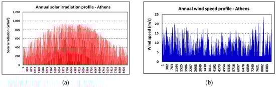
Figure 4.
(a) Annual solar irradiation and (b) wind speed profiles for Athens.
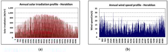
Figure 5.
(a) Annual solar irradiation and (b) wind speed profiles for Heraklion.
5.2. Load Demand Profile
An important parameter during the sizing procedure of a HRES is the load profile. The specific load profile examined as a case study concerned a remote off-grid consumer (four-member dwelling for household use), with average energy requirements equal to 9.45 kWhe/day. It is worth noting that the specific load profile is interlinked only with the concerned dwelling’s electricity consumption, which in turn is not correlated with the building’s thermal loads and consequently its geometrical characteristics. The system sizing is dictated by the relevant hourly peak power demand, equal to 1.52 kWe. Figure 6 depicts the pertinent annual load profile.
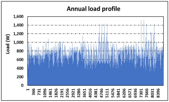
Figure 6.
Annual load profile used for the simulations.
5.3. System Configuration
The architecture of the HRES consists of WT generators, PV modules, and battery banks connected to a common DC (Direct Current) busbar. An inverter electrifies the AC (Alternating Current) load (connected to the AC busbar), also acting as a charge controller for the lead-acid battery banks. The schematic overview of the electric circuit used for the simulations is presented in Figure 7.

Figure 7.
Electric circuit used for the simulations.
5.4. Economic Parameters
Table 2 depicts the system economic parameters which are imported into each software in order to conduct the pertinent analysis, while Table 3 presents the HRES components economic parameters.
Table 2.
System parameters considered for economic analysis.
Table 3.
HRES components economic parameters.
5.5. Optimisation Targets
Economic and power reliability optimisation targets were selected and as consequence different sets of results have been derived. The economic targets aim at minimisation of LCOE and NPC, while the power reliability targets aim at 100% coverage of consumer’s energy demand. The simulation results were accumulated in dedicated Tables for further processing.
Three of the reliability indicators analysed in Section 4 (LOPSP, LA and EUE) were examined, considered as the most widely adopted. These were calculated by the Equations (18)–(20) as:
5.6. Simulation Scenarios
For the evaluation of the selected software, nine different combinations of the previous meteorological data were used as input parameters and simulated with an hourly time step as case studies. Table 4 presents all combinations taken into consideration.
Table 4.
RES potentials combinations.
6. Simulation Results
6.1. System Sizing for Optimum Financial Cost
The results of sizing and financial parameters obtained by the simulation of the examined HRES for optimum financial cost are accumulated in Table 5, Table 6, Table 7 and Table 8.
Table 5.
Simulation results of selected software for the sizing parameters of the HRES examined for optimum financial cost.
Table 6.
Simulation results of the selected software for the energy distribution of the HRES examined for optimum financial cost.
Table 7.
Simulation results of the selected software for unmet load and battery banks’ autonomy of the HRES examined for optimum financial cost.
Table 8.
Simulation results of the selected software for LCOE and NPC of the HRES examined for optimum financial cost.
The following remarks can be concluded:
- iHOGA maintains the total nominal wind power (except for scenario 9) and the batteries bank’s capacity constant as well as their pertinent contribution to load requirement. The strategy opted by the software consists of the diversification of the solar power appropriately to respond to load variation. In contrast, HOMER Pro depicts a diversified dispatch strategy. The software maintains only the total nominal wind power as a constant, whereas both the solar power and also the batteries bank’s capacities are diversified. Moreover, it is worth noting that for scenarios 1 and 4 (where low wind potential is present) HOMER Pro has opted for only PV panels and batteries to satisfy the load demand.
- The PV contribution generated by iHOGA is smaller than the relevant one generated by HOMER Pro for all scenarios examined. On the other hand, HOMER Pro has opted for smaller battery banks’ capacities to satisfy the load requirements in comparison to iHOGA. This is also visualised in the smaller values of batteries bank’s autonomy achieved with HOMER Pro compared to iHOGA.
- For all scenarios examined, HOMER Pro, compared to iHOGA, generates greater volumes of excess energy (ranging from 2 to over 13 times). The previous remark can be principally ascribed to the straightforward control strategy that iHOGA has adopted [11].
With regards to resources allocation, the smaller flexibility noted by iHOGA is the root cause of the greater amounts of annual unmet load compared to the pertinent ones noted by HOMER Pro. To be more precise, the annual unmet load values generated by iHOGA are 1.15 to approximately 17 times greater than the pertinent values generated by HOMER Pro. This fact also affects the variation between the power reliability indicators calculations. The discrepancies between the values calculated for the power reliability indicators LOPSP, LA and EUE are visualised in Figure 8, Figure 9 and Figure 10, respectively, on the basis of the simulation results of the selected simulation software.
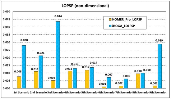
Figure 8.
HOMER Pro and iHOGA LOPSP discrepancies for the 9 scenarios.

Figure 9.
HOMER Pro and iHOGA LA discrepancies for the 9 scenarios.
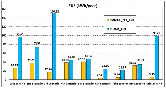
Figure 10.
HOMER Pro and iHOGA EUE discrepancies for the 9 scenarios.
Power reliability indicators are substantially affected by the higher amounts of annual unmet load generated by iHOGA for all scenarios examined. This fact results in greater levels of autonomy and smaller amounts of unserved energy (or energy excess) for the standalone configuration examined. It is also noteworthy that both software tools attained LA values greater than 95.6% for all scenarios examined. Thus, when power reliability optimisation targets are set, HOMER Pro, owing to its dispatch strategy, can be considered more preferable than iHOGA. When financial optimisation constraints are set as a priority, the opposite is valid.
6.2. System Sizing for Optimum Load Coverage
Table 9, Table 10 and Table 11 accumulate the simulation results from HOMER Pro and iHOGA for the sizing and financial parameters of the HRES examined for optimum load coverage.
Table 9.
Optimum load coverage simulation results for the HRES sizing parameters from HOMER Pro and iHOGA.
Table 10.
Optimum load coverage simulation results for the energy distribution of the HRES from HOMER Pro and iHOGA.
Table 11.
Optimum load coverage simulation results of HOMER Pro and iHOGA for LCOE and NPC of the HRES examined.
The following remarks can be concluded:
- As is also valid for the simulations for optimum financial cost, iHOGA maintains the total nominal wind power (except for scenario 5) and the batteries bank’s capacity constant as their pertinent contribution to load demand. The software has opted for the appropriate diversification of solar power to respond to load variation. In contrast, HOMER Pro presents a different dispatch strategy. The software retains constant only the total nominal wind power (except for Scenario 1) and diversifies both the battery banks’ capacities as well as the solar power.
- All energy resources are included in the configurations that have been generated by both software, contrary to the relevant simulations for optimum financial cost.
- The PV contribution generated by iHOGA is greater than the relevant one generated by HOMER Pro for all scenarios examined, as opposed to simulations carried out for optimum financial cost. Furthermore, HOMER Pro has opted for smaller battery banks’ capacities to satisfy the load requirements.
- In 5 out of 9 scenarios (except Scenarios 1, 2, 5 and 7), iHOGA, compared to HOMER Pro, generated smaller amounts of excess energy.
6.3. Comparison of Simulation Results
Table 12 and Table 13 perform a comparison of the simulation results between HOMER Pro, iHOGA and ESA for the nine scenarios examined for optimum financial cost.
Table 12.
Comparison of the optimum financial cost simulation results generated by the three software tools for the sizing parameters.
Table 13.
Comparison of the optimum financial cost simulation results generated by the three software tools for the energy distribution.
The following remarks can be concluded:
- ESA was selected to cover the load demand only with WTs for all scenarios examined. The greater capacity of WTs that resulted from the software simulations has also increased the relevant amount of energy delivered by WTs, compared to the two commercial software examined.
- For all scenarios examined, the battery banks’ capacities generated by ESA are greater than the pertinent ones generated by HOMER Pro. Contrarily, iHOGA generated greater values for the battery banks’ capacities than ESA (except for Scenarios 4 and 5).
- Excluding Scenario 8, the excess energy generated by HOMER Pro is greater than the one generated by ESA. Moreover, iHOGA generated smaller values of excess energy than ESA for all scenarios examined.
7. Discussion
Results from any software shall always be addressed with intrinsic constraints in mind. Familiarity and technical expertise of the software’s user determine to a high extent the simulations’ outcome, necessitating their evaluation with due objectivity. Moreover, the software’s accuracy is enhanced by the quality of data imported and their pertinent detail [107,108]. Due to the fact that the simulations performed were based on hourly distributions of solar irradiation and wind speed, they are considered as the most appropriate input data for the analysis of a pertinent project. Furthermore, the reliability of the findings also depends on the diversity of the case studies examined. The HRES configuration adopted for the simulations was validated against configurations utilised in relevant published studies [10].
As concluded, optimum resource allocation plays the most crucial role for rational compromise between optimisation criteria. The overall findings of the present work research present great interest when compared with existing studies in the literature and pinpoint the requirement for further research. Table 14 aggregates the similarities and discrepancies noted between the present work’s results and three pertinent case studies [11,109,110].
Table 14.
Similarities and discrepancies between the literature and the current research work.
Valuable conclusions could be drawn if the simulations of the current research were repeated via a combination of power reliability and environmental constraints. Moreover, most grid-connected systems are optimised under financial criteria. Thus, of paramount importance would be to repeat the current simulations considering grid-connected instead of standalone HRES and evaluate the pertinent results using the power reliability indicators presented. Furthermore, a variable electrical load could be examined and a relevant sensitivity analysis could be issued for that purpose, contributing to a thorough clarification of the optimisation process.
The gap between modelling capabilities and emerging technologies (or technologies not yet explored in great detail, such as tidal and wave energy) requires ceaseless, long-lasting research and development efforts in the scientific domain of HRES for simulations of increased accuracy. In this context, DSM, load control, financial planning, and forecasting techniques should be incorporated in the HRES operational control. The implied optimised planning can achieve further reduction in the HRES cost. It is noteworthy that the optimisation results shall always consider the maximum penetration limit of wind energy generation into the electricity grid, especially in isolated regions with weak electricity infrastructure.
Energy storage is considered as a prerequisite for the efficient integration of renewable energy into the electricity grids and in this context, there is a constant tendency of novel technologies to appear. Some of them can even be combined to comply with the recommended criteria set by the grid operators for the integration of renewable energy and the quality of power supplied to consumers (Grid Codes). Thus, extended simulations of HRES configurations including different energy storage technologies could be another aspect of long-term work. In addition, the pertinent results can be incorporated into the existing control strategies to boost the percentage of renewable energy injected into the electricity grid. Pareto-based multi-objective optimisation techniques and heuristic approaches could be implemented for that purpose.
Finally, the outputs of control algorithms up to now have been used as a benchmark database for various commercial simulation software. Real-time interactive optimisation algorithms together with ANN are considered the future dominants of the grid junctions’ energy flux. Their behaviour should be investigated and efforts should be made to convert the optimal control strategy from benchmark use to real-time use, adopting respective modelling techniques.
8. Conclusions
The lack of an extended comparison between the selected, most used, commercial software for HRES optimisation was the motivating force for the present work. Several studies were published in the last decade concerning both grid-connected and standalone electrification projects during which the optimum configuration was foraged through various versions of HOMER and at a second level with RETScreen. However, only a tiny minority of them had attempted to clarify, via comparison of simulations, the control strategy adopted from HOMER and iHOGA in relevant projects in order to identify the strong points as also the repercussions of each one on the decision-making.
The current research has realised a review of the theoretical techniques and the software developed for optimising HRES projects. Moreover, it has focused on the various categories of assessment indicators which could serve as optimisation constraints. An important originality imported was that simulations were conducted for nine representative scenarios with one in-house (ESA Microgrid Simulator) and two commercial (HOMER Pro and iHOGA) HRES simulation tools in order to clarify their sensitivity. Special attention was paid to the hourly based elaborate energy balance evaluation for the proposed configuration. Economic and power reliability optimisation targets were selected, being the root cause of different sets of results. The percentage contribution of each renewable energy source, the volume of excess energy generated, and the relevant volume of unmet load were accumulated in dedicated Tables. In this way, they provided responses for the RES that becomes premium by each software and the adopted pertinent dispatch strategy. Subsequently, the selected power reliability indicators were used as the basis for the evaluation of the results.
Finally, a theoretical discussion of the results’ validity was carried out and suggestions for future research work, aiming mainly to incorporate emerging technologies into the current control schemes and render them more efficient, have been carried out.
Author Contributions
Conceptualisation, K.A.K.; methodology, K.A.K.; software, P.T.; validation, K.A.K.; formal analysis, K.A.K. and P.T.; investigation, K.A.K. and P.T.; resources, K.A.K. and P.T.; data curation, P.T.; writing—original draft preparation, P.T.; writing—review and editing, K.A.K.; visualisation, K.A.K. and P.T.; supervision, K.A.K.; project administration, K.A.K.; All authors have read and agreed to the published version of the manuscript.
Funding
This research received no external funding.
Institutional Review Board Statement
Not applicable.
Informed Consent Statement
Not applicable.
Acknowledgments
The authors would like to thank Rodolfo Dufo-López of the University of Zaragoza for his valuable assistance during the simulations with iHOGA software.
Conflicts of Interest
The authors declare no conflict of interest.
Abbreviations
The following abbreviations are used in this manuscript:
| ABC | Artificial Bee Colony |
| AC | Alternating Current |
| AHP | Analytical Hierarchy Process |
| AI | Artificial Intelligence |
| ANN | Artificial Neural Networks |
| CAES | Compressed Air Energy Storage |
| DC | Direct Current |
| DOD | Depth of Discharge |
| DSM | Demand Side Management |
| EPBT | Energy Payback Time |
| ESA | Energy Systems Analysis |
| EUE | Expected Unserved Energy |
| GA | Genetic Algorithms |
| HOMER | Hybrid Optimisation of Multiple Energy Resources |
| HRES | Hybrid Renewable Energy System |
| iHOGA | improved Hybrid Optimisation by Genetic Algorithms |
| LA | Level of Autonomy |
| LOPSP | Loss Of Power Supply Probability |
| LCOE | Levelised Cost Of Electricity |
| MCS | Monte Carlo Simulations |
| NPC | Net Present Cost |
| NREL | National Renewable Energy Laboratory |
| O & M | Operation & Maintenance |
| Probability Density Function | |
| PLC | Probability of Load Curtailment |
| PSO | Particle Swarm Optimisation |
| PV | Photovoltaic |
| RES | Renewable Energy Sources |
| SA | Simulating Annealing |
| SOC | State Of Charge |
| TLBO | Teaching-Learning Based Optimisation |
| TMY | Typical Meteorological Year |
| WT | Wind Turbine |
References
- Erdinc, O.; Uzunoglu, M. Optimum design of hybrid renewable energy systems: Overview of different approaches. Renew. Sustain. Energy Rev. 2012, 16, 1412–1425. [Google Scholar] [CrossRef]
- Kavadias, K.; Triantafyllou, P. Wind-based stand-alone hybrid energy systems. In Reference Module in Earth Systems and Environmental Sciences; Elsevier: Oxford, UK, 2021. [Google Scholar]
- Kavadias, K.A. Modern Solar Map of Greece with Application in Hybrid Renewable Energy Systems (Available in Greek Only). Ph.D. Thesis, University of Ioannina, Ioannina, Greece, January 2016. [Google Scholar]
- Sinha, S.; Chandel, S.S. Review of software tools for hybrid renewable energy systems. Renew. Sustain. Energy Rev. 2014, 33, 192–205. [Google Scholar] [CrossRef]
- Kavadias, K.A. Stand-alone, hybrid systems. In Comprehensive Renewable Energy; Sayigh, A., Kaldellis, J.K., Eds.; Elsevier: Oxford, UK, 2012; Volume 2, pp. 623–656. [Google Scholar]
- Bhandari, B.; Lee, K.T.; Lee, G.Y.; Chso, Y.M.; Ahn, S.H. Optimization of Hybrid Renewable Energy Power Systems: A Review. Int. J. Precis. Eng. Manuf. Green Technol. 2015, 2, 99–112. [Google Scholar] [CrossRef]
- Turcotte, D.; Ross, M.; Sheriffa, F. Photovoltaic hybrid system sizing and simulation tools: Status and needs. In Proceedings of the PV Horizon: Workshop on Photovoltaic Hybrid Systems, Montreal, QC, Canada, 10 September 2001; pp. 1–10. [Google Scholar]
- Subramanian, A.S.R.; Gundersen, T.; Adams, T.A., II. Modeling and Simulation of Energy Systems: A Review. Processes 2018, 6, 238. [Google Scholar] [CrossRef] [Green Version]
- Acuña, L.G.; Padilla, R.V.; Santander-Mercado, A.R. Measuring reliability of hybrid photovoltaic-wind energy systems: A new indicator. Renew. Energy 2017, 106, 68–77. [Google Scholar] [CrossRef]
- Al-Falahi, M.D.A.; Jayasinghe, S.D.G.; Enshaei, H. A review on recent size optimisation methodologies for standalone solar and wind hybrid renewable energy system. Energy Convers. Manag. 2012, 143, 252–274. [Google Scholar] [CrossRef]
- Saiprasad, N.; Kalam, A.; Zayegh, A. Comparative Study of Optimisation of HRES using HOMER and iHOGA Software. J. Sci. Ind. Res. 2018, 77, 677–683. [Google Scholar]
- Kumar, P. Analysis of hybrid systems: Software tools. In Proceedings of the IEEE International Conference on Advances in Electrical, Electronics, Information, Communication and Bio-Informatics (AEEICB16), Chennai, India, 27–28 February 2016. [Google Scholar]
- Diaf, S.; Diaf, D.; Belhamel, M.; Haddadi, M.; Louche, A. A methodology for optimal sizing of autonomous hybrid PV/wind system. Energy Policy 2007, 35, 5708–5718. [Google Scholar] [CrossRef] [Green Version]
- Connolly, D.; Lund, H.; Mathiesen, B.V.; Leahy, M. A review of computer tools for analysing the integration of renewable energy. Appl. Energy 2010, 87, 1059–1082. [Google Scholar] [CrossRef]
- Zhou, W.; Yang, H.; Fang, Z. A novel model for photovoltaic array performance prediction. Appl. Energy 2007, 84, 1187–1198. [Google Scholar] [CrossRef]
- Ashok, S. Optimised model for community-based hybrid energy system. Renew. Energy 2007, 32, 1155–1164. [Google Scholar] [CrossRef]
- Kondili, E. Design and performance optimisation of stand-alone and hybrid wind energy systems. In Stand-Alone and Hybrid Wind Energy Systems: Technology, Energy Storage and Applications; Kaldellis, J.K., Ed.; Woodhead Publishing Series in Energy: Oxford, UK, 2010; pp. 81–101. [Google Scholar]
- HOMER Pro. Available online: https://www.homerenergy.com/products/pro (accessed on 19 July 2019).
- iHOGA. Available online: http://ihoga.unizar.es/en (accessed on 21 October 2019).
- Piraeus University of Applied Sciences. Technology Innovation for the Local Scale, Optimum Integration of Battery Energy Storage, TILOS, Innovation Project LCE-08-2014: Local/Small Scale Storage. D7.1 The Validated Microgrid Simulator; The TILOS Consortium: Egaleo, Greece, 2017; pp. 1–48. [Google Scholar]
- Ghofrani, M.; Hosseini, N.N. Optimizing hybrid renewable energy systems: A review. In Sustainable Energy-Technological Issues, Applications and Case Studies; Zobaa, A.F., Afifi, S., Pisica, I., Eds.; Intech: Rijeka, Croatia, 2016; Chapter 8; pp. 161–176. [Google Scholar]
- Tina, G.M.; Gagliano, S.; Raiti, S. Hybrid solar/wind power system probabilistic modelling for long-term performance assessment. Elsevier Sol. Energy 2006, 80, 578–588. [Google Scholar] [CrossRef]
- Khatod, D.K.; Pant, V.; Sharma, J. Analytical Approach for Well-Being Assessment of Small Autonomous Power Systems with Solar and Wind Energy Sources. IEEE Trans. Energy Convers. 2010, 25, 535–545. [Google Scholar] [CrossRef]
- Zhou, W.; Lou, C.; Li, Z.; Lu, L.; Yang, H. Current status of research on optimum sizing of stand-alone hybrid solar–wind power generation systems. Appl. Energy 2010, 87, 380–389. [Google Scholar] [CrossRef]
- Li, J.; Wei, W.; Xiang, J. A Simple Sizing Algorithm for Stand-Alone PV/Wind/Battery Hybrid Microgrids. Energies 2012, 5, 5307–5323. [Google Scholar] [CrossRef] [Green Version]
- Chedid, R.; Rahman, S. Unit sizing and control of hybrid wind-solar power systems. IEEE Trans. Energy Convers. 1997, 12, 79–85. [Google Scholar] [CrossRef] [Green Version]
- Huneke, F.; Henkel, J.; Benavides González, J.A.; Erdmann, G. Optimisation of hybrid off-grid energy systems by linear programming. Energy Sustain. Soc. 2012, 2, 1–19. [Google Scholar] [CrossRef] [Green Version]
- De, A.R.; Musgrove, L. The optimization of hybrid energy conversion systems using the dynamic programming model–Rapsody. Int. J. Energy Res. 1988, 12, 447–457. [Google Scholar] [CrossRef]
- Bakirtzis, A.G.; Gavanidou, E.S. Optimum operation of a small autonomous system with unconventional energy sources. Electr. Power Syst. Res. 1992, 23, 93–102. [Google Scholar] [CrossRef]
- Konak, A.; Coit, D.W.; Smith, A.E. Multi-objective optimization using genetic algorithms: A tutorial. Reliab. Eng. Syst. Saf. 2006, 91, 992–1007. [Google Scholar] [CrossRef]
- Ming, M.; Wang, R.; Zha, Y.; Zhang, T. Multi-Objective Optimization of Hybrid Renewable Energy System Using an Enhanced Multi-Objective Evolutionary Algorithm. Energies 2017, 10, 674. [Google Scholar] [CrossRef] [Green Version]
- Singh, R.; Bansal, R.C.; Singh, A.R.; Naidoo, R. Multi-objective optimization of hybrid renewable energy system using reformed electric system cascade analysis for islanding and grid connected modes of operation. IEEE Access 2018, 6, 47332–47354. [Google Scholar] [CrossRef]
- Saramourtsis, A.C.; Bakirtzis, A.G.; Dokopoulos, P.S.; Gavanidou, E.S. Probabilistic evaluation of the performance of wind-diesel energy systems. IEEE Trans. Energy Convers. 1994, 9, 743–752. [Google Scholar] [CrossRef]
- Karaki, S.H.; Chedid, R.B.; Ramadan, R. Probabilistic Performance Assessment of Autonomous Solar-Wind Energy Conversion Systems. IEEE Trans. Energy Convers. 1999, 14, 766–772. [Google Scholar] [CrossRef]
- Dagdougui, H.; Minciardi, R.; Ouammi, A.; Robba, M.; Sacile, R. Modelling and control of a hybrid renewable energy system to supply demand of a “Green” building. Energy Convers. Manag. 2012, 64, 351–363. [Google Scholar] [CrossRef]
- Bhandari, B.; Poudel, S.R.; Lee, K.-T.; Ahn, S.-H. Mathematical Modeling of Hybrid Renewable Energy System: A Review on Small Hydro-Solar-Wind Power Generation. Int. J. Precis. Eng. Manuf. Green Technol. 2014, 1, 157–173. [Google Scholar] [CrossRef]
- Zhang, L.; Barakat, G.; Yassine, A. Deterministic Optimization and Cost Analysis of Hybrid PV/Wind/Battery/Diesel Power System. Int. J. Renew. Energy Res. 2012, 2, 686–696. [Google Scholar]
- Borowy, B.S.; Salameh, Z.M. Methodology for Optimally Sizing the Combination of a Battery Bank and PV Array in a Wind/PV Hybrid System. IEEE Trans. Energy Convers. 1996, 11, 367–375. [Google Scholar] [CrossRef]
- Markvart, T. Sizing of hybrid photovoltaic-wind energy systems. Sol. Energy 1996, 57, 277–281. [Google Scholar] [CrossRef]
- Ramoji, S.K.; Rath, B.B.; Kumar, D.V. Optimization of Hybrid PV Wind Energy System Using Genetic Algorithm (GA). Int. J. Eng. Res. Appl. 2014, 4, 29–37. [Google Scholar]
- Rao, R.V.; Savsani, V.J.; Vakharia, D.P. Teaching–learning-based optimization: A novel method for constrained mechanical design optimization problems. Comput. Aided Des. 2011, 43, 303–315. [Google Scholar] [CrossRef]
- Kalogirou, S.A. Optimization of solar systems using artificial neural-networks and genetic algorithms. Appl. Energy 2004, 77, 383–405. [Google Scholar] [CrossRef]
- Alzahrani, A.; Ferdowsi, M.; Shamsi, P.; Dagli, C.H. Modeling and Simulation of Microgrid. Procedia Comput. Sci. 2017, 114, 392–400. [Google Scholar] [CrossRef]
- Saharia, B.J.; Brahma, H.; Sarmah, N. A review of algorithms for control and optimization for energy management of hybrid renewable energy systems. J. Renew. Sustain. Energy 2018, 10, 1–33. [Google Scholar]
- Kennedy, V.; Eberhart, R. Particle swarm optimization. In Proceedings of the ICNN’95-IEEE International Conference on Neural Networks, Perth, WA, Australia, 27 November–1 December 1995; pp. 1942–1948. [Google Scholar]
- Geleta, D.K.; Manshahia, M.S. Artificial bee colony-based optimization of hybrid wind and solar renewable energy system. In Handbook of Research on Energy-Saving Technologies for Environmentally-Friendly Agricultural Development; Kharchenko, V., Vasant, P., Eds.; IGI Global: Hershey, PA, USA, 2019; Chapter 17; pp. 429–453. [Google Scholar]
- Eltamaly, A.M.; Mohamed, M.A.; Al-Saud, M.S.; Alolah, A.I. Load management as a smart grid concept for sizing and designing of hybrid renewable energy systems. Eng. Optim. 2017, 49, 1813–1828. [Google Scholar] [CrossRef]
- Clerc, M. Particle Swarm Optimization; ISTE Ltd.: London, UK, 2006. [Google Scholar]
- Lehmann, S.; Rutter, I.; Wagner, D.; Wagner, F. A simulated-annealing-based approach for wind farm cabling. In Proceedings of the 8th International Conference on Future Energy Systems, Shatin, Hong Kong, 16–19 May 2017; pp. 203–215. [Google Scholar]
- Yang, K.; Kwak, G.; Cho, K.; Huh, J. Wind farm layout optimization for wake effect uniformity. Energy 2019, 183, 983–995. [Google Scholar] [CrossRef]
- Dong, W.; Li, Y.; Xiang, J. Optimal Sizing of a Stand-Alone Hybrid Power System Based on Battery/Hydrogen with an Improved Ant Colony Optimization. Energies 2016, 9, 785. [Google Scholar] [CrossRef]
- Suhane, P.; Rangnekar, S.; Mittal, A. Optimal Sizing of Hybrid Energy System using Ant Colony Optimization. Int. J. Renew. Energy Res. 2014, 4, 683–688. [Google Scholar]
- Ringkjøb, H.K.; Haugan, P.M.; Solbrekke, I.M. A review of modelling tools for energy and electricity systems with large shares of variable renewables. Renew. Sustain. Energy Rev. 2018, 96, 440–459. [Google Scholar] [CrossRef]
- Santarelli, M.; Pellegrino, D. Mathematical optimization of a RES-H2 plant using a black box algorithm. Renew. Energy 2005, 30, 493–510. [Google Scholar] [CrossRef]
- Yang, M.; Chen, C.; Que, B.; Zhou, Z.; Yang, Q. Optimal placement and configuration of hybrid energy storage system in power distribution networks with distributed photovoltaic sources. In Proceedings of the 2018 2nd IEEE Conference on Energy Internet and Energy System Integration (EI2), Beijing, China, 20–22 October 2018; pp. 1–6. [Google Scholar]
- Upadhyay, S.; Sharma, M.P. A review on configurations, control and sizing methodologies of hybrid energy systems. Renew. Sustain. Energy Rev. 2014, 38, 47–63. [Google Scholar] [CrossRef]
- Ganguly, P.; Kalam, A.; Zayegh, A. Design an optimum standalone hybrid renewable energy system for a small town at Portland, Victoria using iHOGA. In Proceedings of the 2017 Australasian Universities Power Engineering Conference (AUPEC), Melbourne, Australia, 19–22 November 2017; pp. 1–6. [Google Scholar]
- Al-Sheikh, H.; Moubayed, N. An overview of simulation tools for renewable applications in power systems. In Proceedings of the 2012 2nd International Conference on Advances in Computational Tools for Engineering Applications (ACTEA), Beirut, Lebanon, 12–15 December 2012; pp. 257–261. [Google Scholar]
- Lundsager, P.; Bindner, H.; Clausen, N.-E.; Frandsen, S.; Hansen, L.H.; Hansen, J.C. Isolated Systems with Wind Power; Risø National Laboratory: Roskilde, Denmark, 2001; pp. 1–72.
- International Energy Agency. World-Wide Overview of Design and Simulation Tools for Hybrid PV Systems; International Energy Agency: Paris, France, 2011.
- Lambert, T.; Gilman, P.; Lilienthal, P. Micropower system modeling with HOMER. In Integration of Alternative Sources of Energy; Farret, F.A., Simões, M.G., Eds.; John Wiley & Sons, Inc.: Hoboken, NJ, USA, 2006; Chapter 15; pp. 379–418. [Google Scholar]
- Hirschberg, S.; Bauer, C.; Burgherr, P.; Dones, R.; Simons, A.; Schenler, W.; Bachmann, T.; Gallego Carrera, D.; Maupu, V.; Lecointe, C.; et al. Deliverable n° D3.2–RS 2b: Final set of sustainability criteria and indicators for assessment of electricity supply options. In NEEDS-New Energy Externalities Developments for Sustainability; Project no: 502687; Paul Scherrer Institut: Villigen, Switzerland, 2008. [Google Scholar]
- Polatidis, H.; Haralambopoulos, D.; Munda, G.; Vreeker, R. Selecting an Appropriate Multi-Criteria Decision Analysis Technique for Renewable Energy Planning. Energy Sources Part B 2006, 1, 181–193. [Google Scholar] [CrossRef]
- Afgan, N.H.; Carvalho, M.G. Sustainability assessment of a hybrid energy system. Energy Policy 2008, 36, 2903–2910. [Google Scholar] [CrossRef]
- Liu, G.; Rasul, M.G.; Amanullah, M.T.O.; Khan, M.M.K. AHP and fuzzy assessment based sustainability indicator for hybrid renewable energy system. In Proceedings of the 2010 20th Australasian Universities Power Engineering Conference, Christchurch, New Zealand, 5–8 December 2010; pp. 1–6. [Google Scholar]
- Santoyo-Castelazo, E.; Azapagic, A. Sustainability assessment of energy systems: Integrating environmental, economic and social aspects. J. Clean. Prod. 2014, 80, 119–138. [Google Scholar] [CrossRef]
- Wang, R.; Lam, C.M.; Hsu, S.C.; Chen, J.H. Life cycle assessment and energy payback time of a standalone hybrid renewable energy commercial microgrid: A case study of Town Island in Hong Kong. Appl. Energy 2019, 250, 760–775. [Google Scholar] [CrossRef]
- Dufo-López, R.; Bernal-Agustin, J.L. Design and control strategies of PV-Diesel systems using genetic algorithms. Sol. Energy 2005, 79, 33–46. [Google Scholar] [CrossRef]
- Gudelj, A.; Krčum, M. Simulation and Optimization of Independent Renewable Energy Hybrid System. Trans. Marit. Sci. 2013, 1, 28–35. [Google Scholar] [CrossRef] [Green Version]
- Heylen, E.; Deconinck, G.; Van Hertem, D. Review and classification of reliability indicators for power systems with a high share of renewable energy sources. Renew. Sustain. Energy Rev. 2018, 97, 554–568. [Google Scholar] [CrossRef]
- Chaer, R.; Zeballos, R.; Uturbey, W.; Casaravilla, G. Simenerg: A novel tool for designing autonomous electricity systems. In Proceedings of the European Community Wind Energy Conference (ECWEC), Lübeck-Travemünde, Germany, 8–12 March 1993; pp. 330–333. [Google Scholar]
- Yazdanpanah, M.-A. Modeling and sizing optimization of hybrid photovoltaic/wind power generation system. J. Ind. Eng. Int. 2014, 49, 1–14. [Google Scholar] [CrossRef] [Green Version]
- Xydis, G. On the exergetic capacity factor of a wind-Solar power generation system. J. Clean. Prod. 2013, 47, 437–445. [Google Scholar] [CrossRef] [Green Version]
- Puri, A. Optimally sizing battery storage and renewable energy sources on an off-grid facility. In Proceedings of the 2013 IEEE Power & Energy Society (PES) General Meeting, Vancouver, BC, Canada, 21–25 July 2013; pp. 1–5. [Google Scholar]
- Singh, R.; Bansal, R. Optimization of an autonomous hybrid renewable energy system using reformed electric system cascade analysis. IEEE Trans. Ind. Inform. 2019, 15, 399–409. [Google Scholar] [CrossRef] [Green Version]
- Kashefi Kaviani, A.; Riahy, G.H.; Kouhsari, S.M. Optimal design of a reliable hydrogen-based stand-alone wind/PV generating system, considering component outages. Renew. Energy 2009, 34, 2380–2390. [Google Scholar] [CrossRef]
- Wu, Y.K.; Chang, S.M. Review of the optimal design on a hybrid renewable energy system. In Proceedings of the 2016 1st Asia Conference on Power and Electrical Engineering (ACPEE 2016), Bangkok, Thailand, 20–22 March 2016; pp. 1–7. [Google Scholar]
- Shrestha, G.B.; Goel, L. A study on optimal sizing of stand-alone photovoltaic stations. IEEE Trans. Energy Convers. 1998, 13, 373–378. [Google Scholar] [CrossRef]
- Chen, H.-C. Optimum capacity determination of stand-alone hybrid generation system considering cost and reliability. Elsevier Appl. Sci. 2013, 103, 155–164. [Google Scholar] [CrossRef]
- Boroujeni, H.F.; Eghtedari, M.; Abdollahi, M.; Behzadipour, E. Calculation of generation system reliability index: Loss of Load Probability. Life Sci. J. 2012, 9, 4903–4908. [Google Scholar]
- Al-Ashwal, A.M.; Moghram, I.S. Proportion assessment of combined PV-Wind generating systems. Renew. Energy 1997, 10, 43–51. [Google Scholar] [CrossRef]
- Celik, A.N. Techno-economic analysis of autonomous PV-wind hybrid energy systems using different sizing methods. Energy Convers. Manag. 2003, 44, 1951–1968. [Google Scholar] [CrossRef]
- Medjoudj, R.; Bediaf, H.; Aissani, D. Power system reliability: Mathematical models and applications. In System Reliability; Volosencu, C., Ed.; IntechOpen: London, UK, 2017; Chapter 15; pp. 279–298. [Google Scholar]
- Billinton, R.; Li, W. Reliability Assessment of Electric Power Systems Using Monte Carlo Methods, 1st ed.; Plenum Press: New York, NY, USA, 1994. [Google Scholar]
- Maghraby, H.A.M.; Shwehdi, M.H.; Al-Bassam, G.K. Probabilistic Assessment of Photovoltaic (PV) Generation Systems. IEEE Trans. Power Syst. 2002, 17, 205–208. [Google Scholar] [CrossRef]
- Yang, H.X.; Lu, L.; Burnett, J. Weather data and probability analysis of hybrid photovoltaic–wind power generation systems in Hong Kong. Renew. Energy 2003, 28, 1813–1824. [Google Scholar] [CrossRef]
- Ganguly, P.; Kalam, A.; Zayegh, A. Solar–wind hybrid renewable energy system: Current status of research on configurations, control, and sizing methodologies. In Hybrid-Renewable Energy Systems in Microgrids, Integration, Developments and Control; Hina Fathima, A., Palanisamy, K., Mekhilef, S., Eds.; Woodhead Publishing Series in Energy: Oxford, UK, 2018; Chapter 12; pp. 219–248. [Google Scholar]
- Moriana, I.; San Martin, I.; Sanchis, P. Wind-photovoltaic hybrid systems design. In Proceedings of the 2010 2nd International Symposium on Power Electronics Electrical Drives Automation and Motion (SPEEDAM), Pisa, Italy, 14–16 June 2010; pp. 610–615. [Google Scholar]
- Maleki, A.; Pourfayaz, F. Optimal sizing of autonomous hybrid photovoltaic/wind/battery power system with LPSP technology by using evolutionary algorithms. Sol. Energy 2015, 115, 471–483. [Google Scholar] [CrossRef]
- Hina Fathima, A.; Palanisamy, K. Optimization in microgrids with hybrid energy systems–A review. Renew. Sustain. Energy Rev. 2015, 45, 431–446. [Google Scholar] [CrossRef]
- Hafez, A.A.; Hatata, A.Y.; Aldl, M.M. Optimal sizing of hybrid renewable energy system via artificial immune system under frequency stability constraints. J. Renew. Sustain. Energy 2019, 11, 015905. [Google Scholar] [CrossRef]
- Zahboune, H.; Zouggar, S.; Krajacic, G.; Sabev Varbanov, P.; Elhafyani, M.; Ziani, E. Optimal hybrid renewable energy design in autonomous system using Modified Electric System Cascade Analysis and Homer software. Energy Convers. Manag. 2016, 126, 909–922. [Google Scholar] [CrossRef]
- Luna-Rubio, R.; Trejo-Perea, M.; Vargas-Vázquez, D.; Ríos-Moreno, G.J. Optimal sizing of renewable hybrids energy systems: A review of methodologies. Sol. Energy 2012, 86, 1077–1088. [Google Scholar] [CrossRef]
- Shirvani, M.; Memaripour, A.; Abdollahi, M.; Salimi, A. Calculation of generation system reliability index: Expected Energy Not Served. Life Sci. J. 2012, 9, 3443–3448. [Google Scholar]
- Al-Shaalan, A.M. Reliability evaluation of power systems. In Reliability and Maintenance-an Overview of Cases; Kounis, L.D., Ed.; IntechOpen: London, UK, 2019; Chapter 1; pp. 1–25. [Google Scholar]
- Aien, M.; Biglari, A.; Rashidinejad, M. Probabilistic reliability evaluation of hybrid wind-photovoltaic power systems. In Proceedings of the 2013 21st Iranian Conference on Electrical Engineering (ICEE), Mashhad, Iran, 14–16 May 2013; pp. 1–6. [Google Scholar]
- Wang, L.; Singh, C. Compromise between cost and reliability in optimum design of an autonomous hybrid power system using mixed-integer PSO algorithm. In Proceedings of the 2007 International Conference on Clean Electrical Power, Capri, Italy, 21–23 May 2007; pp. 682–689. [Google Scholar]
- Garcia, R.S.; Weisser, D. A wind–diesel system with hydrogen storage: Joint optimisation of design and dispatch. Renew. Energy 2006, 31, 2296–2320. [Google Scholar] [CrossRef]
- Jahanbani, F.; Riahy, G.H. Optimum design of a hybrid renewable energy system. In Renewable Energy-Trends and Applications; Nayeripour, M., Khesti, M., Eds.; Intech: Rijeka, Croatia, 2011; Chapter 11; pp. 231–250. [Google Scholar]
- Navaeefard, A.; Moghaddas-Tafreshi, S.M.; Barzegari, M.; Shahrood, A.J. Optimal sizing of distributed energy resources in microgrid considering wind energy uncertainty with respect to reliability. In Proceedings of the 2010 IEEE International Energy Conference, Manama, Bahrain, 18–22 December 2010; pp. 820–821. [Google Scholar]
- Bashir, M.; Sadeh, J. Size optimization of new hybrid stand-alone renewable energy system considering a reliability index. In Proceedings of the 2012 11th International Conference on Environment and Electrical Engineering, Venice, Italy, 18–25 May 2012; pp. 1–6. [Google Scholar]
- Baghaee, H.R.; Mirsalim, M.; Gharehpetian, G.B.; Talebi, H.A. Reliability/cost-based multi-objective Pareto optimal design of stand-alone wind/PV/FC generation microgrid system. Energy 2016, 115, 1022–1041. [Google Scholar] [CrossRef]
- Fockens, S.; van Wijk, A.J.M.; Turkenburg, W.C.; Singh, C. Reliability analysis of generating systems including intermittent sources. Int. J. Electr. Power Energy Syst. 1992, 14, 2–8. [Google Scholar] [CrossRef]
- Singh, C.; Bagchi, A. Reliability analysis of power systems incorporating renewable energy sources. In Proceedings of the 16th National Power Systems Conference, Hyderabad, India, 15–17 December 2010; pp. 43–49. [Google Scholar]
- Singh, R.; Bansal, R.C.; Tiwari, N. Optimization and comparison of autonomous renewable energy system based on ESCA technique. In Proceedings of the IEEE International WIE Conference on Electrical and Computer Engineering (WIECON-ECE), Dehradun, India, 18–19 December 2017; pp. 21–24. [Google Scholar]
- NASA Prediction of Worldwide Energy Resources. Available online: https://power.larc.nasa.gov (accessed on 20 July 2019).
- Tozzi, P.; Jo, J.H. A comparative analysis of renewable energy simulation tools: Performance simulation model vs. system optimization. Renew. Sustain. Energy Rev. 2017, 80, 390–398. [Google Scholar] [CrossRef]
- Yoro, K.O.; Daramola, M.O.; Sekoai, P.T.; Wilson, U.N.; Eterigho-Ikelegbe, O. Update on current approaches, challenges, and prospects of modeling and simulation in renewable and sustainable energy systems. Renew. Sustain. Energy Rev. 2021, 150, 1–15. [Google Scholar] [CrossRef]
- Ataei, A.; Nedaei, M.; Rashidi, R.; Yoo, C. Optimum design of an off-grid hybrid renewable energy system for an office building. J. Renew. Sustain. Energy 2015, 7, 1–25. [Google Scholar] [CrossRef]
- Alkarrami, F.; Iqbal, T.; Pope, K. Optimal sizing of a stand-Alone hybrid energy system for water pumping in Sirte, Libya. In Proceedings of the 2016 IEEE Electrical Power and Energy Conference (EPEC), Ottawa, ON, Canada, 12–14 October 2016; pp. 1–5. [Google Scholar]


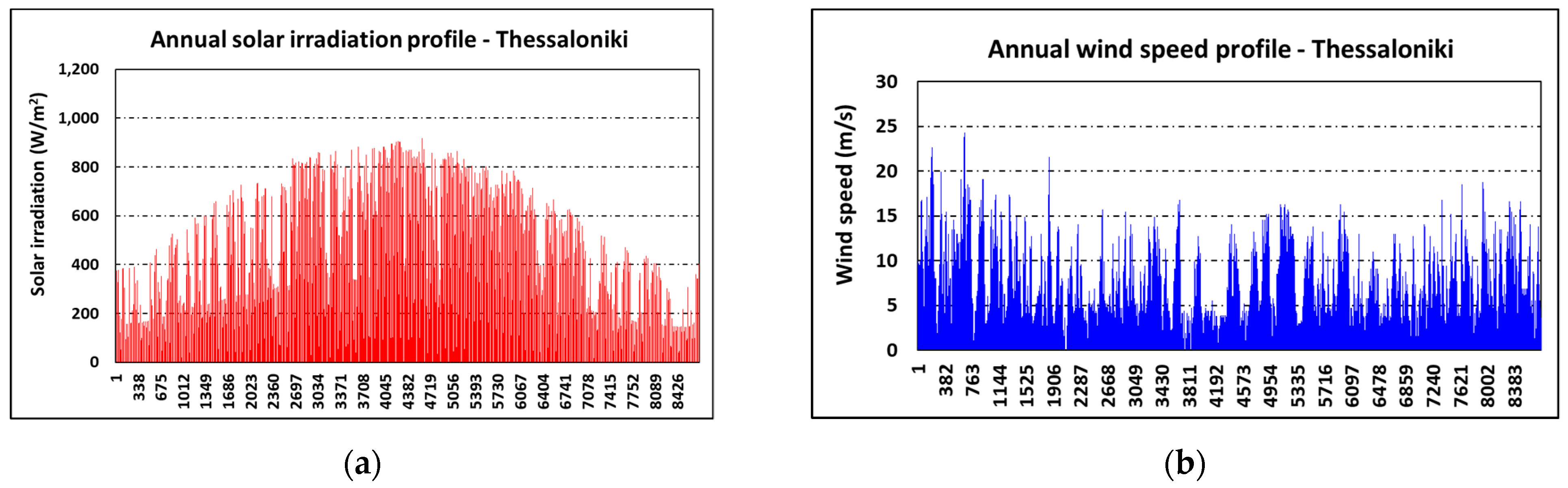
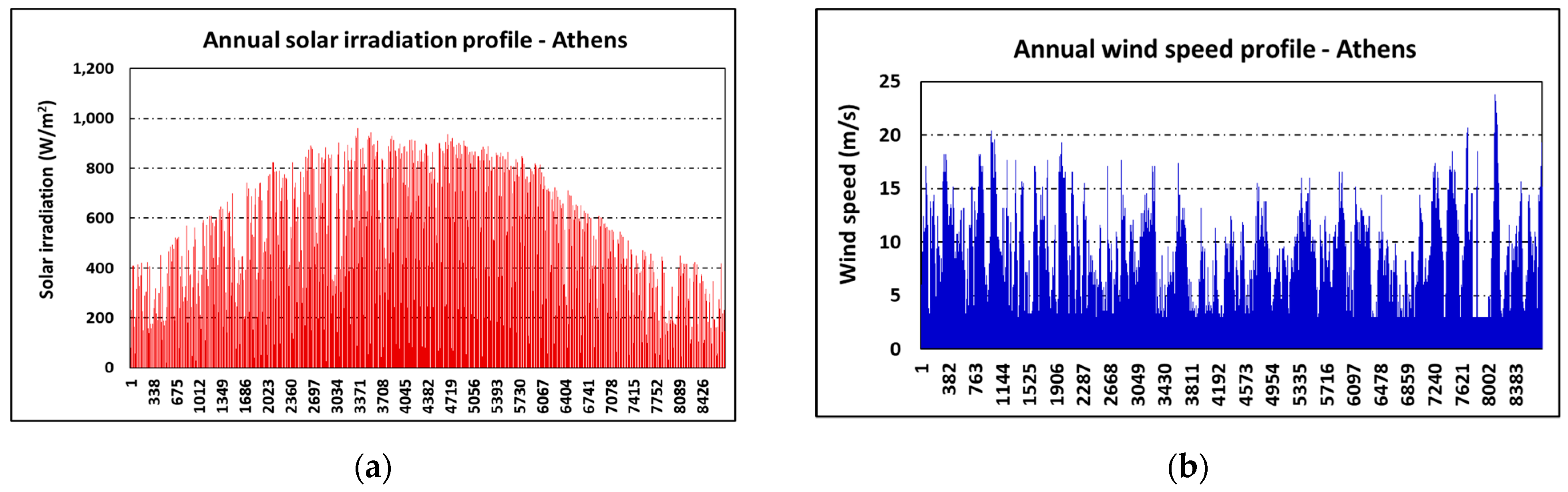
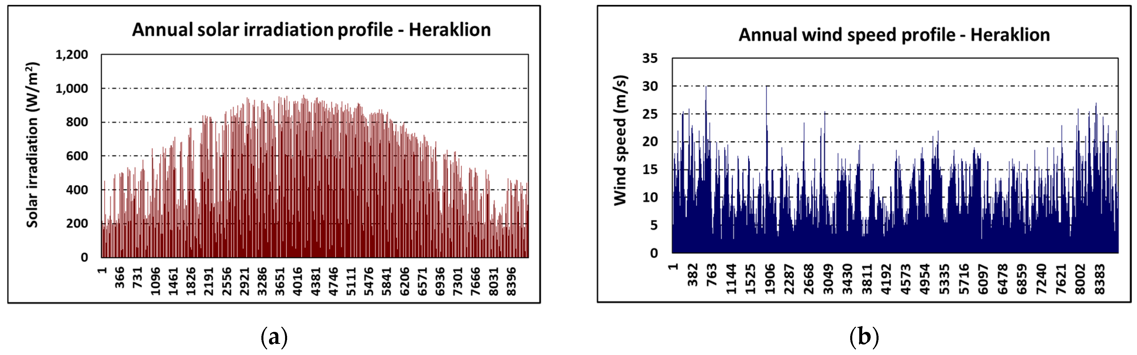
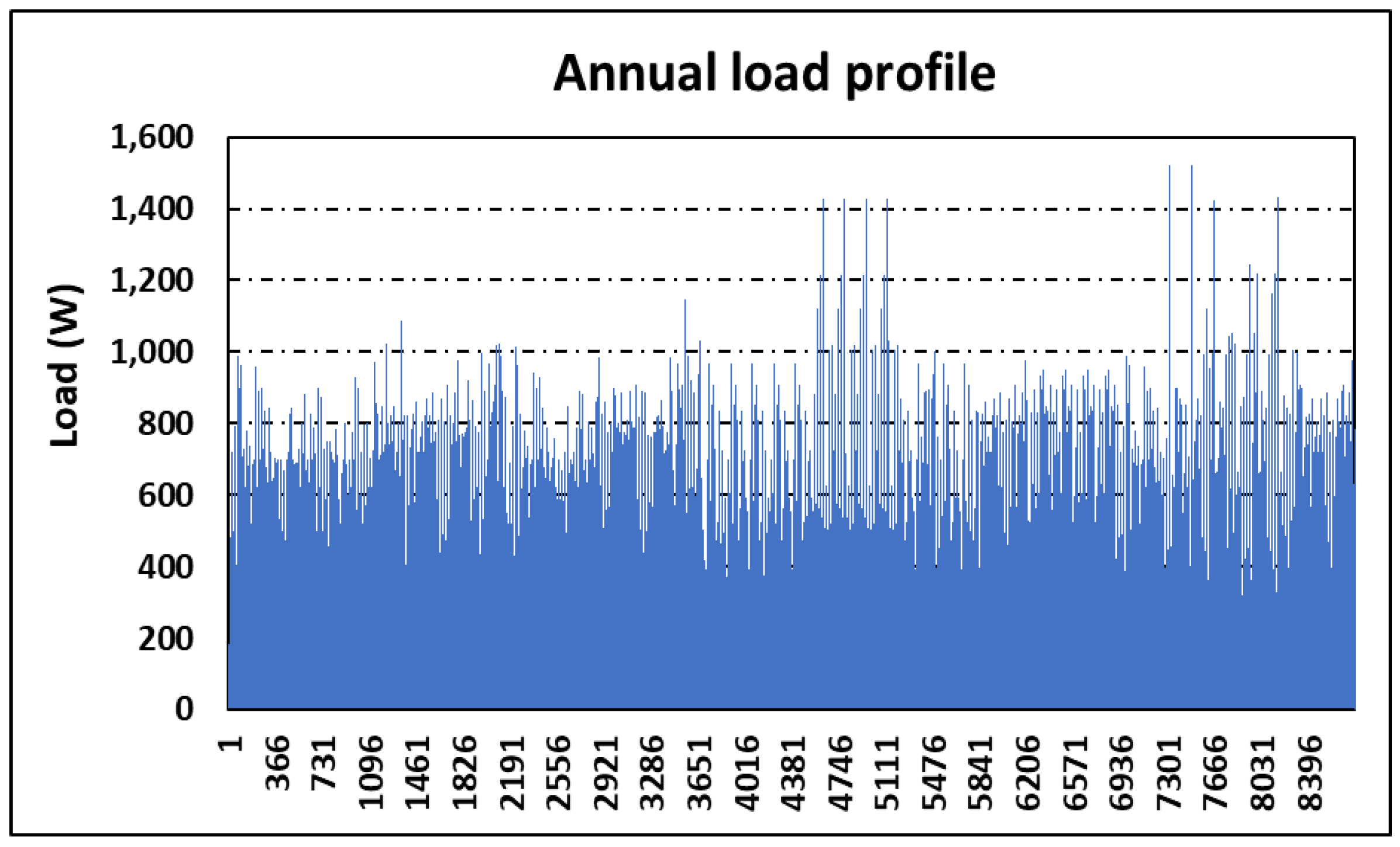
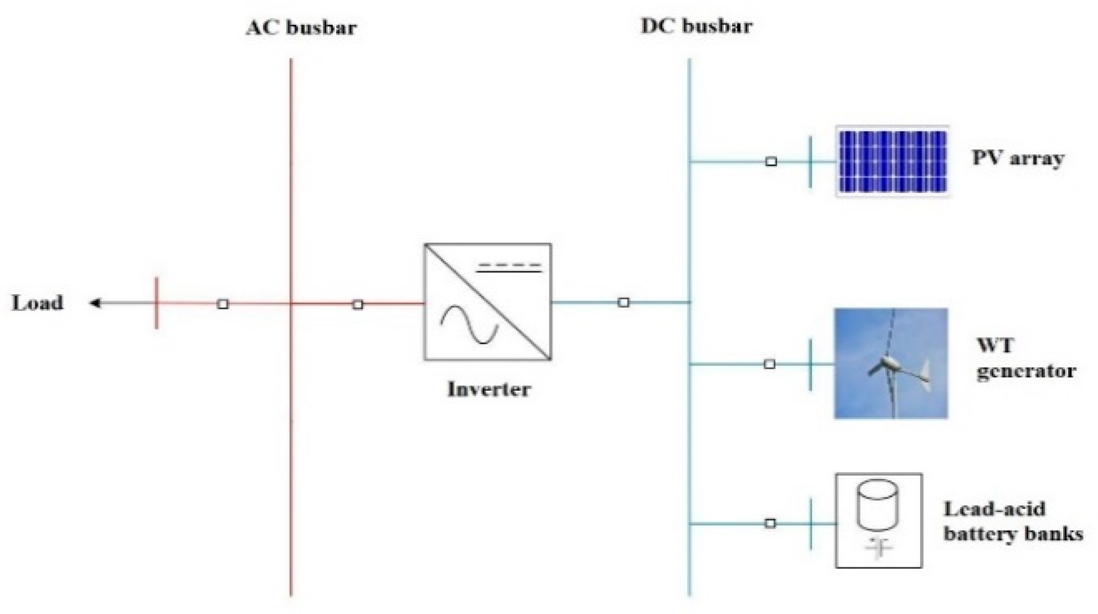
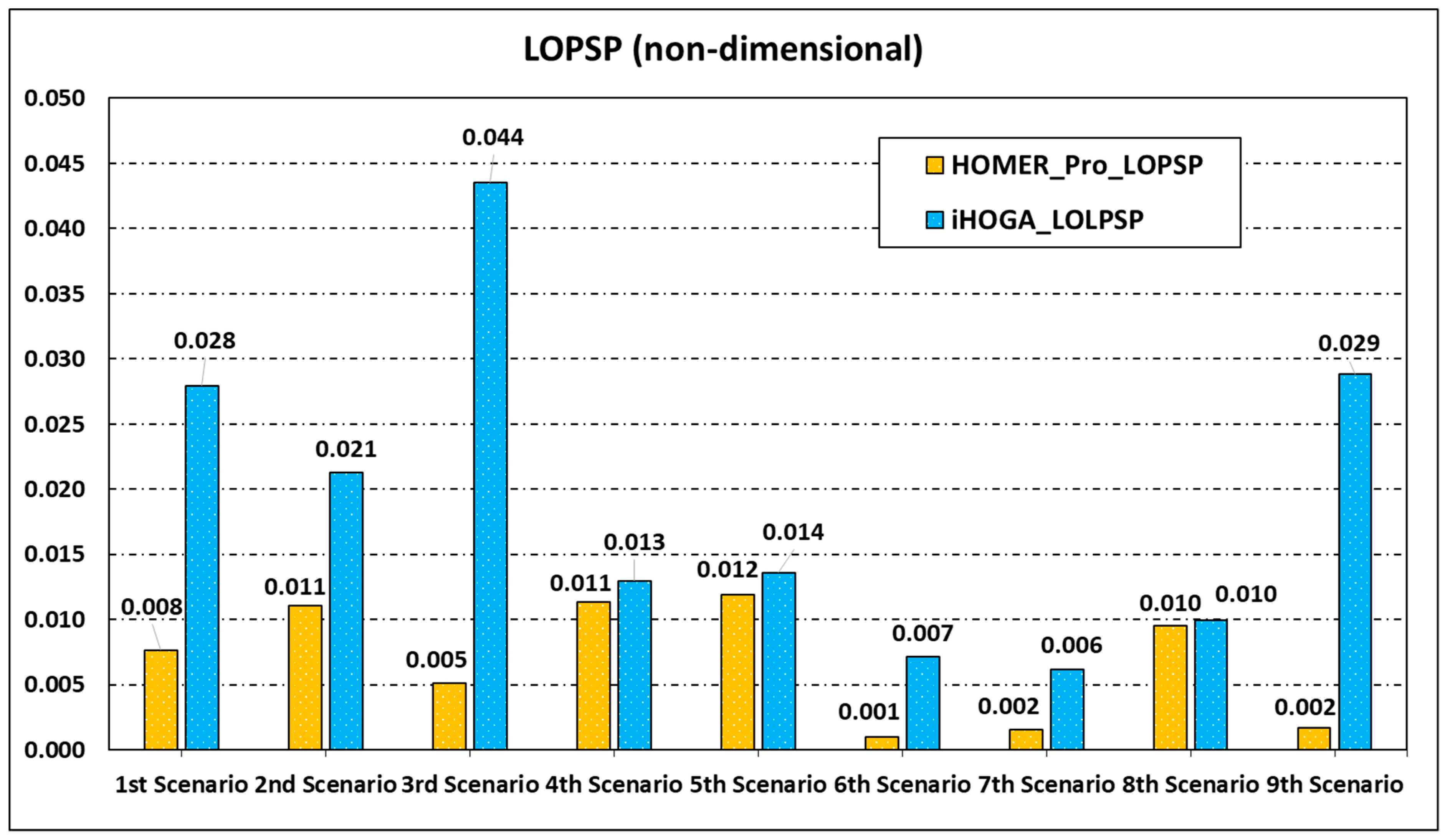
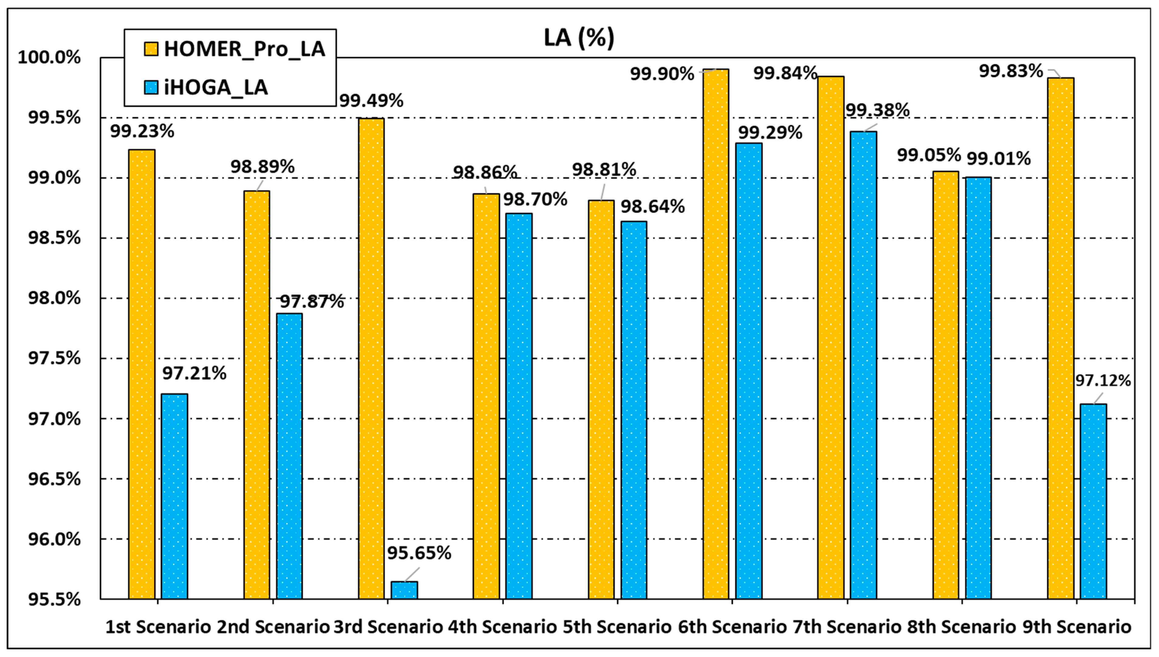

Publisher’s Note: MDPI stays neutral with regard to jurisdictional claims in published maps and institutional affiliations. |
© 2021 by the authors. Licensee MDPI, Basel, Switzerland. This article is an open access article distributed under the terms and conditions of the Creative Commons Attribution (CC BY) license (https://creativecommons.org/licenses/by/4.0/).