Numerical Investigation on Propagation Behaviors of a Three-Dimensional Fracture Network Coupled with Microseismicity in Fractured Shale Reservoirs

Abstract

The formation mechanism and propagation behaviors of a three-dimensional hydraulic fracture network in fractured shale reservoirs remain unclear, especially when the scale of hydraulic fractures is much larger than that of natural fractures. In this study, taking the well XH in the Longmaxi shale reservoir in the Sichuan Basin, China as an example, we develop a fully three-dimensional numerical model for hydraulic fracturing coupled with microseismicity based on the discrete lattice method. We introduce a randomly generated discrete fracture network into the proposed model and explore the formation mechanism of the hydraulic fracture network under the condition that the hydraulic fractures are much larger than natural fractures in scale. Moreover, microseismic events are inversely synthesized in the numerical model, which allows the evolution of the fracture network to be monitored and evaluated quantitatively. In addition, we analyze the effects of injection rate, horizontal stress difference, and fluid viscosity on fracture propagation. Our results show that when the scale of hydraulic fractures is much larger than that of natural fractures, the fracture morphology of “main hydraulic fractures + complex secondary fractures” is mainly formed. We find that a high injection rate can not only create a complex fracture network, but also improve the uniform propagation of multi-cluster fractures and enhance far-field stimulation efficiency. Optimizing the horizontal wellbore intervals with low horizontal stress differences as the sweet spots of hydraulic fracturing is also beneficial to improve the stimulation efficiency. For zones with a large number of natural fractures, it is recommended to use an injection schedule with high viscosity fluid early and low viscosity fluid late to allow the hydraulic fractures to propagate to the far-field to maximize the stimulation effect.

1. Introduction

Due to the influence of tectonic movement and sedimentary environment, a large number of weak geological planes exist in unconventional reservoirs such as natural fractures, bedding planes, and faults [1,2,3,4,5,6,7]. When hydraulic fractures encounter natural fractures, a variety of complex propagation behaviors can occur, such as crossing, offsetting, and being arrested [8,9,10,11,12]. These complex interactions lead to the formation of complex fractures and even fracture networks. Additionally, recent sampling of the fracture core for testing also suggests that propagation behavior at a local scale can be extremely complex [13]. While these complexities cannot be easily modeled in a traditional sense, it may be relevant to consider how they may have an impact on propagation characteristics. Therefore, simulating the propagation behaviors of fractures for unconventional reservoirs has become one of the current research focuses [14,15,16].

The cohesive zone model (CZM) can not only characterize the initiation and propagation of hydraulic fractures, but can also describe the tangential flow and normal filtration of fracturing fluid. Because of these advantages, the simulations of a two-dimensional fracture network [17,18,19] and a three-dimensional fracture network [20,21] based on the cohesive zone model have been carried out, and the effects of injection rate, cementation strength, and natural fracture distribution on the hydraulic fracture network have been discussed. The displacement discontinuity method (DDM) has been widely used in simulating complex hydraulic fractures or fracture networks due to its high computational efficiency [22,23,24]. In addition, significant effort towards modeling fracture networks has been devoted to other advanced methods including the embedded discrete fracture model [25,26], the extended finite element method [27,28], and peridynamics [29]. In laboratory experiments, Zhang et al. (2021) studied the initiation, deflection, and propagation of hydraulic fractures interacting with multiple natural fractures in different directions using triaxial fracturing experiments by embedding a closed cemented pre-existing fracture network in the specimens [30]. They found four interaction behaviors between hydraulic fractures and multiple natural fractures. Liu et al. (2018) used specimens with randomly generated natural fractures by placing small cement pieces and found that the main hydraulic fracture geometry is either a main multi-branched fracture with a fracture network, a main multi-branched fracture, or just a single main fracture [31]. Tan et al. (2017) conducted true-triaxial fracturing experiments on specimens recovered from layered shale outcrops, found complex fracture morphology from specimens with developed bedding planes, and obtained the favorable conditions for creating a complex fracture network [32].

These studies have improved the understanding of complex fracture propagation in fractured unconventional reservoirs under the influence of various geological and engineering factors and have provided theoretical support for the design and optimization of fracturing operation parameters in the field. However, most of these numerical studies have been focused on two-dimensional or pseudo-three-dimensional modeling, without considering fracture height growth. Furthermore, it is generally assumed that the scale of natural fractures, especially in the fracture height, is equivalent to the scale of hydraulic fractures in the existing research. These are the possible reasons that the propagation of the fracture network obtained from numerical simulations differs from the actual situation, which is not beneficial to fracture optimization in unconventional reservoirs.

In this study, taking the well XH in the Sichuan basin, China as an example, we establish a three-dimensional geomechanical model for hydraulic fracturing in fractured shale reservoirs coupled with microseismicity based on the discrete lattice method. In this model, we introduce a discrete fracture network characterized by randomly distributed natural fractures and explore the formation mechanism of the fracture network with the scale of the hydraulic fracture being much larger than that of a natural fracture. Moreover, microseismic events are inversely synthesized in the fracturing model to monitor the evolution of the fracture network and quantitatively evaluate the propagation behavior. Finally, we systematically examine the effects of injection rate, horizontal stress difference, and fluid viscosity on the propagation behavior of the fracture network.

2. Discrete Lattice Method

The discrete lattice method (Figure 1), which is a commercial version developed by Itasca, is a simplified discrete element method based on the synthetic rock and lattice theory [33,34,35,36,37,38]. The central difference equations used to calculate the translational freedom degrees of the nodes [33,36] are expressed as,

$$\{\begin{array}{c}{\dot{u}}_i^{\left(t+\Delta t/2\right)}={\dot{u}}_i^{\left(t-\Delta t/2\right)}+{\displaystyle \sum }{F}_i^{\left(t\right)}\Delta t/m\\ u_i^{\left(t+\Delta t\right)}=u_i^{\left(t\right)}+{\dot{u}}_i^{\left(t+\Delta t/2\right)}\Delta t\end{array}$$

(1)

where ${\dot{u}}_i^{\left(t\right)}$ and $u_i^{\left(t\right)}$ are the velocity and displacement of component i (i = 1, 3) at time t, respectively; $\sum F_i$ is the sum of all force components i (i = 1, 3) acting on the node with mass m; and Δt is the time step.

The angular velocity ω_i of component i (i = 1, 3) at time t is calculated by the following central difference equation [33,36],

$${\omega }_i^{\left(t+\Delta t/2\right)}={\omega }_i^{\left(t-\Delta t/2\right)}+\frac{\sum M_i^{\left(t\right)}}{I}\Delta t$$

(2)

where $\sum M_i$ is the sum of all moment components acting on the node; and I is the moment of inertia.

The relative displacement of the node is used to calculate the force change of the spring, which is written as [33,36],

$$\{\begin{array}{c}{F}^N\leftarrow F^N+{\dot{u}}^N{k}^N\Delta t\\ F_i{}^s\leftarrow F_i{}^s+{\dot{u}}_i{}^s{k}^s\Delta t\end{array}$$

(3)

where the superscript N represents the normal direction; the superscript S represents the tangential direction; k is the spring stiffness; and F is the spring force.

When the tensile force or shear force of the spring exceeds the maximum allowed by the spring (F^N > F^Nmax or F^S > F^Smax), tensile failure or shear failure occurs, and as a result, micro-fractures are created.

The fluid flow in the pipeline is described by the lubrication equation. The injection rate q along the pipeline from node A to node B is calculated by [33,36],

$$q=\beta k_r\frac{a^3}{12\mu }\left[p^A-p^B+{\rho }_{w}g\left(z^A-z^B\right)\right]$$

(4)

where β is a dimensionless calibration parameter; α is the fracture opening, μ is the fluid viscosity; superscripts A and B represent the node A and B, respectively; p is the fluid pressure; z is the elevation of the node; ρ_w is the fluid density; and g is the gravitational acceleration.

The increment of fluid pressure ΔP for a flow time step Δt_f is calculated as [33,36],

$$\Delta P=\frac{\sum q_i}{V}{\overline{K}}_F\Delta t_f$$

(5)

where ${\overline{K}}_F$ is the apparent fluid bulk modulus; V is the nodal volume; and q_i is the injection rate from the pipeline connected to the node i.

Microseismic events in the discrete lattice method are calculated by the slip of fracture [40],

$$M_0=G\times l_{slip}\times A_{slip}$$

(6)

where M₀ is the seismic moment; G is the shear modulus; l_slip is the sliding length; and A_slip is the sliding area.

The coupling between solid deformation and fluid flow is considered in the discrete lattice method. Fracture permeability depends on fracture opening and matrix deformation, affecting the fluid pressure in the fractures. Changes in fluid pressure affect the matrix deformation and failure of the mechanical model, which is in turn impacted by the matrix deformation.

3. Three-Dimensional Numerical Model of Hydraulic Fracture Network

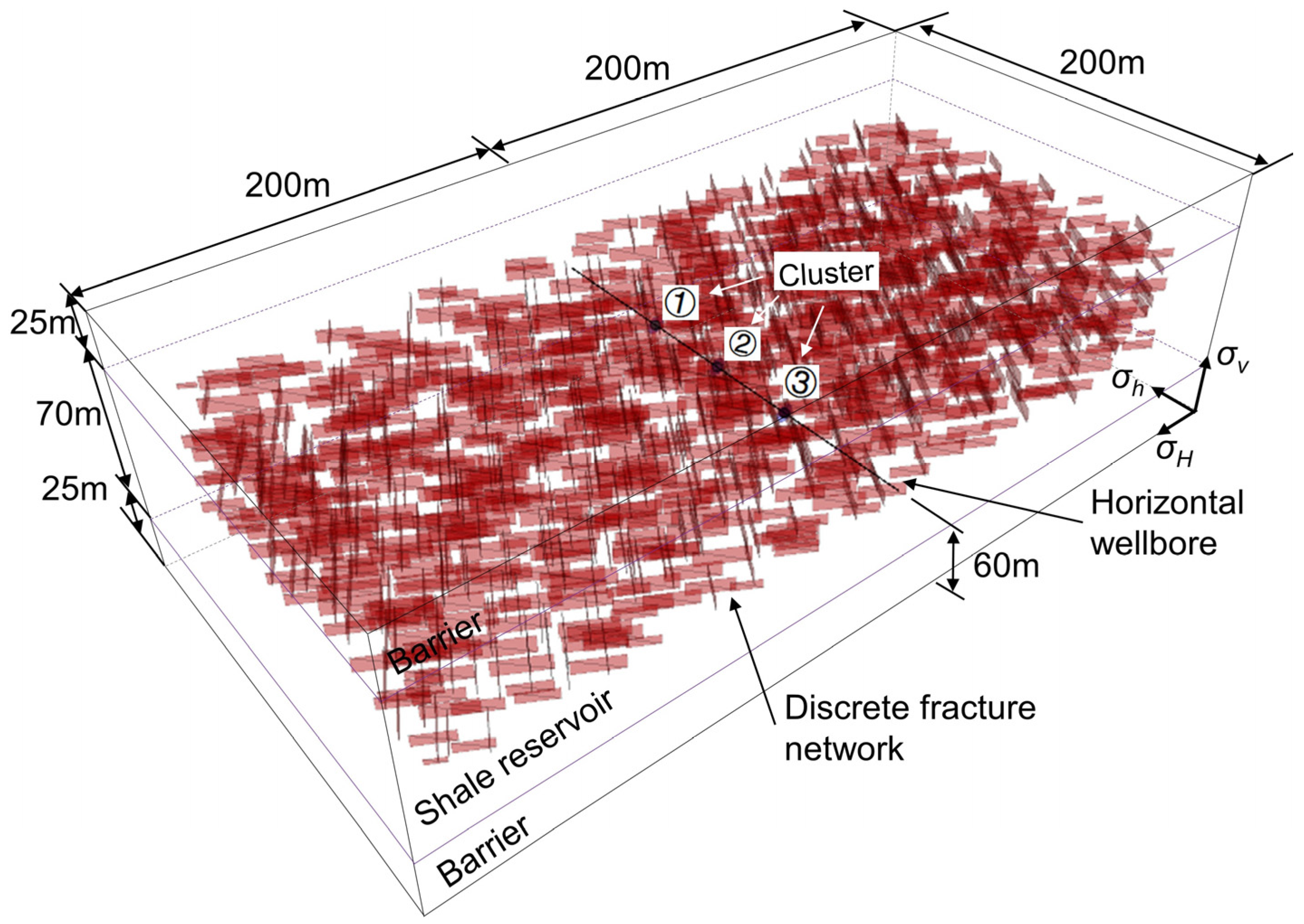
3.1. Engineering Background

The well XH is located in the Sichuan basin, China, and the target shale reservoir is the Longmaxi formation with a thickness of about 70 m. The angle between the strike direction of the well-developed natural fractures and the direction of the maximum horizontal stress is 30°. Slick water with a low viscosity is used as the injection fluid with an injection rate of 13 m³/min. The length of the horizontal wellbore is 1900 m. There are three perforation clusters with a spacing of 30~50 m. The length of each perforation interval is 1 m and the perforation density is 16 holes/m. The helical perforation with a perforation phase angle of 60° is applied. The injection volume for each stage is 1300~1800 m³. Field results show that the productivity of gas wells is increased significantly after hydraulic fracturing, but the increments are different as operating parameters change. Therefore, understanding the impacts of operating parameters such as injection rate, fluid viscosity, and horizontal stress difference on the stimulation effect is important to the design and optimization of parameter control for shale reservoirs.

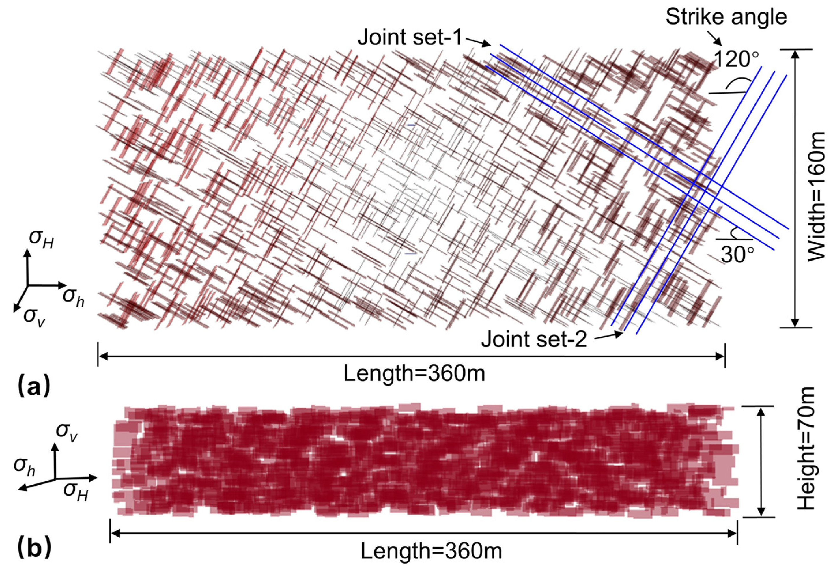
3.2. Establishment of the Three-Dimensional Fracture Network Model

The three-dimensional fracture network model (shown in Figure 2) is built based on the combination of geological parameters (Table 1) and operational parameters (Table 2) of well XH. It is noted that the voronoi tessellation is adopted to generate the mesh in the discrete lattice method. Moreover, a fixed mesh is used, and thus the mesh at the fracture tip does not remesh during the simulation. In addition, the mesh sensity is not considered in our work due to the time-consuming calculation. The initial stresses and stratigraphies are derived from the analysis of well logging data by the field engineers in the PetroChina Southwest Oil & Gas Field Company, Chengdu. The dimension of the model is 200 m × 400 m × 120 m, in which the 70 m thick reservoir is sandwiched between upper and lower barriers of 25 m each. The horizontal wellbore is located in the middle of the reservoir, along with the orientation of the minimum horizontal stress. There are three perforation clusters with a cluster spacing of 40 m. The overburden stress, the maximum and the minimum horizontal stresses are 57.5 MPa, 52.5 MPa, and 47.5 MPa, respectively, and the stress boundary conditions are used for the fracture model.

To consider the effects of natural fracture distribution, the discrete fracture network (Figure 3) is embedded into the shale reservoir (Figure 2). To remove the boundary effects, the dimension of the discrete fracture network is set as 70 m × 160 m × 360 m, smaller than the shale reservoir. A series of 1232 natural fractures are randomly generated to constitute the discrete fracture network. These natural fractures consist of two groups of conjugate joints, one with an angle of 30° between the strike and the maximum horizontal stress direction (joint set-1 in Figure 3a), and the other with an angle of 120° (joint set-2 in Figure 3a). The dip angle of natural fractures is 80°, and the length and height of natural fractures are 6~24 m and 2~8 m, respectively. The tensile strength, cohesion, and internal friction angle are 1.24 MPa, 3.75 MPa, and 25°, respectively [41]. The viscosity of the fracturing fluid is 3 mPa.s, the injection rate is 13 m³/min, and the injection time is 6300 s.

The input data in our numerical model mainly comprises the model size (in the previous paragraph in this Section), the mechanical properties of shale reservoirs (Table 1), and natural fractures (in the previous paragraph in this Section); the petrophysical parameters of shale reservoirs including matrix permeability, porosity, and leak-off coefficient (Table 1); the fracturing fluid properties, e. g., fluid density and fluid viscosity (Table 2); the in situ stresses including formation pore-pressure, overburden stress, and maximum and minimum horizontal stresses (Table 1); and the operational parameters such as injection rate, injection time, perforation parameters, and cluster setting (Table 2).

Table 1. Geological parameters of the shale reservoir.

Parameters	Shale Reservoir
Formation pore pressure (MPa)	29.4
Maximum horizontal principal stress (MPa)	52.5
Minimum horizontal principal stress (MPa)	47.5
Overburden stress (MPa)	57.5
Uniaxial compressive strength (MPa)	200.1
Tensile strength (MPa)	13.16
Poisson’s ratio	0.26
Elastic modulus (GPa)	52.89
Fracture toughness (MPa/m0.5)	0.96
Leak-off coefficient (m/s0.5)	1.2 × 10−4
Matrix permeability (mD)	0.002
Porosity (%)	5

Note: The tensile strength and fracture toughness are derived from Heng et al. (2020) [42].

Table 1. Geological parameters of the shale reservoir.

Parameters	Shale Reservoir
Formation pore pressure (MPa)	29.4
Maximum horizontal principal stress (MPa)	52.5
Minimum horizontal principal stress (MPa)	47.5
Overburden stress (MPa)	57.5
Uniaxial compressive strength (MPa)	200.1
Tensile strength (MPa)	13.16
Poisson’s ratio	0.26
Elastic modulus (GPa)	52.89
Fracture toughness (MPa/m0.5)	0.96
Leak-off coefficient (m/s0.5)	1.2 × 10−4
Matrix permeability (mD)	0.002
Porosity (%)	5

Note: The tensile strength and fracture toughness are derived from Heng et al. (2020) [42].

Table 2. Operational parameters.

Parameters	Value
Number of clusters	3
Cluster spacing (m)	40
Injection rate (m3/min)	13
Fluid viscosity (mPa.s)	3
Fluid density (kg/m3)	1010
Fracturing fluid type	Newtonian fluid
Injection time (s)	6300
Perforation phase angle (°)	60
Perforation density (holes/m)	16

Table 2. Operational parameters.

Parameters	Value
Number of clusters	3
Cluster spacing (m)	40
Injection rate (m3/min)	13
Fluid viscosity (mPa.s)	3
Fluid density (kg/m3)	1010
Fracturing fluid type	Newtonian fluid
Injection time (s)	6300
Perforation phase angle (°)	60
Perforation density (holes/m)	16

In addition, several strategies are applied to reduce the influence of boundary effect on fracture propagation. On one hand, we enlarge the dimension size of the numerical model as much as possible under an allowable calculation-cost, to make the fractures propagate in a relatively small area in the middle of the model. On the other hand, the dimension size of the discrete fracture network (70 m × 160 m × 360 m) is set smaller than the shale reservoir (Figure 2) to mitigate the influence of boundary effects on the discrete fracture network. It is noted that the heterogeneity of the rock properties along the well and across the reservoir is not considered in our current model. The reasons for using homogeneous parameters in our model include: (1) the current fracture model cannot consider the heterogeneity of the reservoir properties, thereby improving our model to consider the reservoir heterogeneity is a promising work in the next step; (2) it is reasonable to adopt homogeneous rock properties in our current research to a certain extent, in that the variation of rock properties of the target reservoir is relatively small for well XH.

The modeling process in the discrete lattice method includes the following steps:

Firstly, the characteristics of natural fractures (such as the fracture strike, dimension size, and mechanical properties) in the target shale reservoir is obtained by the analysis of rock cores and well logging. Then we create the discrete fracture network using the fracture stochastic modeling in the particle flow code (PFC).

Secondly, the discrete fracture network is imported into the three-dimensional fracturing model on the basis of the discrete lattice method to establish the network fracturing model.

Thirdly, the mechanical properties of shale reservoir, fluid properties, and in situ stresses are assigned to the numerical model.

Fourthly, the mechanical equilibrium of the fracturing model is carried out for a certain time (4 s in our simulation) before fluid injection. Only the mechanical calculation for solid is implemented in this process.

Finally, fracturing fluid is forced to be injected into the formation to simulate hydraulic fracturing, which is a fluid-solid coupling process.

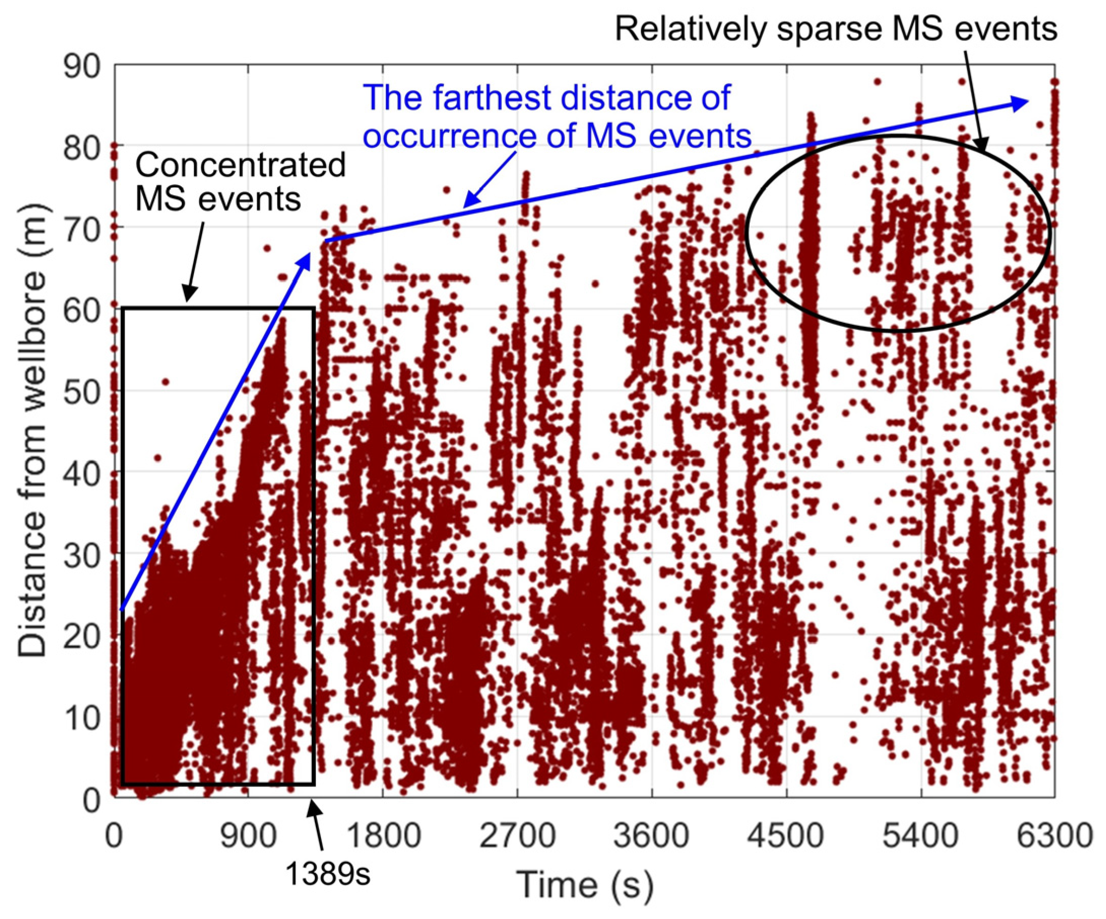
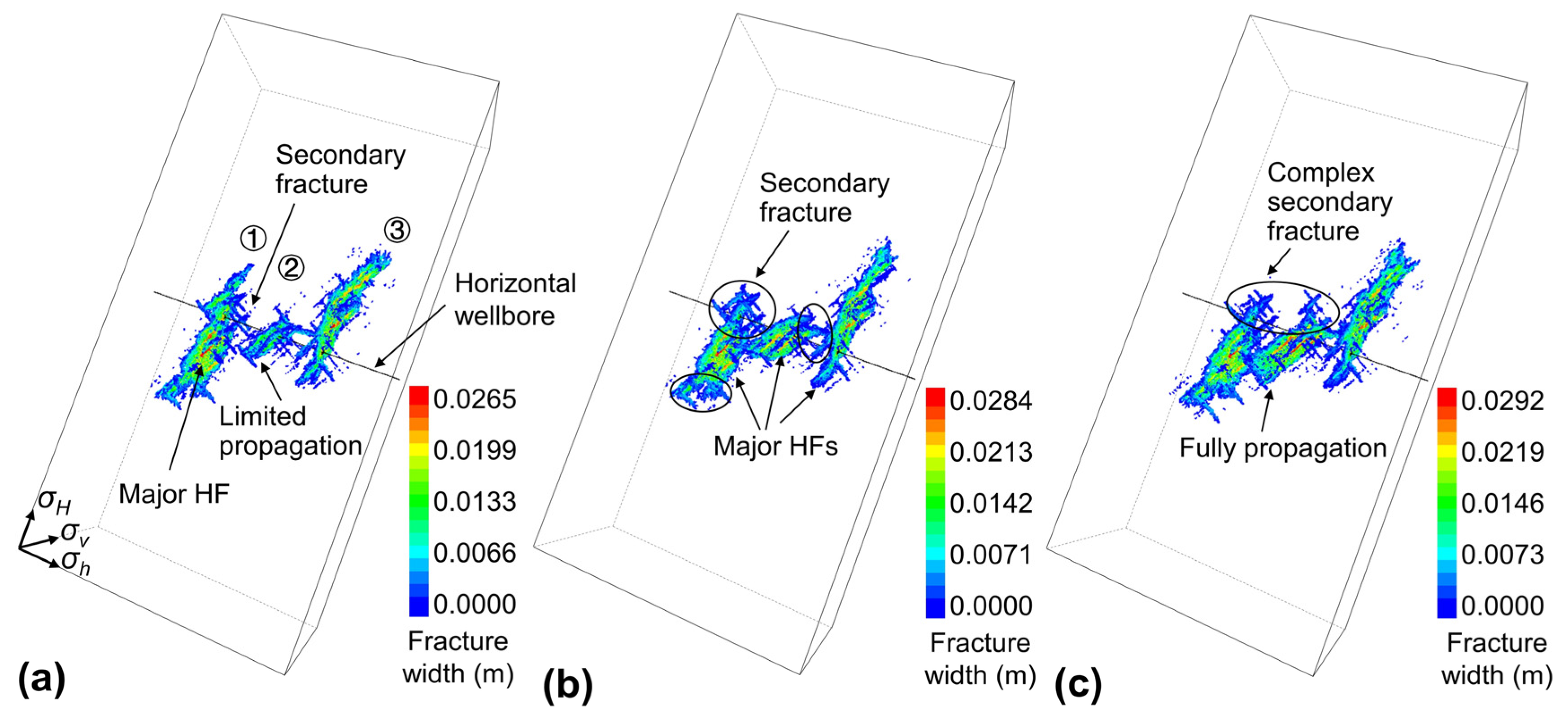
3.3. Numerical Simulation Results and Model Verification

Figure 4 shows the morphologies of the three-dimensional fracture network and the distribution of microseismic events, with an injection time of 6300 s. Complex hydraulic fractures consisting of main hydraulic fractures and secondary multi-branched fractures are formed from all three clusters (Figure 4a). The main hydraulic fractures in the first and third clusters propagate perpendicular to the direction of the minimum horizontal stress, while the main hydraulic fracture in the second cluster deviates from that direction and propagates along the strike direction of joint set-1 due to the impact of natural fractures near the wellbore. This indicates that the propagation of hydraulic fractures is not only controlled by in situ stresses but also affected by natural fractures. The existence of natural fractures, on one hand, affects the propagation direction of the main hydraulic fractures. On the other hand, after hydraulic fractures are connected with natural fractures, natural fractures are activated, resulting in complex secondary fractures.

Figure 4b shows that microseismic events are concentrated in the hydraulic fracture area, indicating that the spatial distribution of microseismic events can characterize the fracture morphology. These microseismic events are called wet events. Therefore, the spatial evolution of the fracture network can be described by the evolution of wet microseismic events. In addition, isolated microseismic events, named dry events, can also be generated beyond the hydraulic fractures [43,44]. There are two types of dry events in our numerical simulation. The first type is a small number of microseismic events that occur on some natural fractures during the initial stage of hydraulic fracturing, represented by blue circles in Figure 4b. These microseismic events are possibly caused by the small dislocation of some natural fractures right after the fluid is injected. The second type are microseismic events that occur at the propagation front of hydraulic fractures, represented by the red circles in Figure 4b. This is because the stress concentration near the fronts of hydraulic fractures causes natural fractures to slip, resulting in these microseismic events.

Microseismic events that occurred at different distances away from the horizontal wellbore are calculated to evaluate the fracture propagation quantitatively, as shown in Figure 5. Microseismic events gradually appear in the farther regions with time. The farthest location of microseismic events exhibits a bilinear trend with time; that is, it increases rapidly in the early stage of fracturing (0~1389 s), but the increment slows down in the later stage of fracturing (1389~6300 s). In addition, microseismic events are densely distributed within 60 m of the near-wellbore region in the early stage of fracturing (0~1389 s). In the later stage of fracturing (1389~6300 s), microseismic events are distributed throughout the whole area, including the near-wellbore area and far-field area. In other words, many microseismic events still appear in the near-wellbore area, indicating that a large amount of fracturing fluid is consumed by fluid filtration or reactivation of natural fractures in the near-wellbore area. This phenomenon leads to a significant reduction in the volume of fracturing fluid used to stimulate the far-field reservoir, which is the reason for the lack of microseismic events in the far-field region in the later stage of fracturing, as illustrated in Figure 5.

Figure 6 shows the comparison of injection pressures between the numerical simulation and fracturing practice at well XH in the field. The evolution of the injection pressure obtained by the numerical simulation is generally consistent with that of the field injection pressure. For example, the extension pressures of the two curves exhibit similarly frequent fluctuations, which are related to the formation of complex fractures. In addition, the breakdown pressure obtained from the numerical simulation is 77.11 MPa, which is 3.02 MPa (4.08%) higher than that obtained from field fracturing (74.09 MPa). Moreover, the maximum difference in extension pressure between the numerical simulation and the field fracturing is 5.28 MPa (7.55%). These comparisons show that the proposed numerical model of hydraulic fracturing can reliably describe the propagation of the fracture network in well XH in the fractured shale reservoir. In addition, it is noted that we do not compare the field microseismic results with numerical microseismic results, in that microseismic monitoring is not conducted in the field for the well XH.

4. Propagation Behaviors of Three-Dimensional Fracture Network

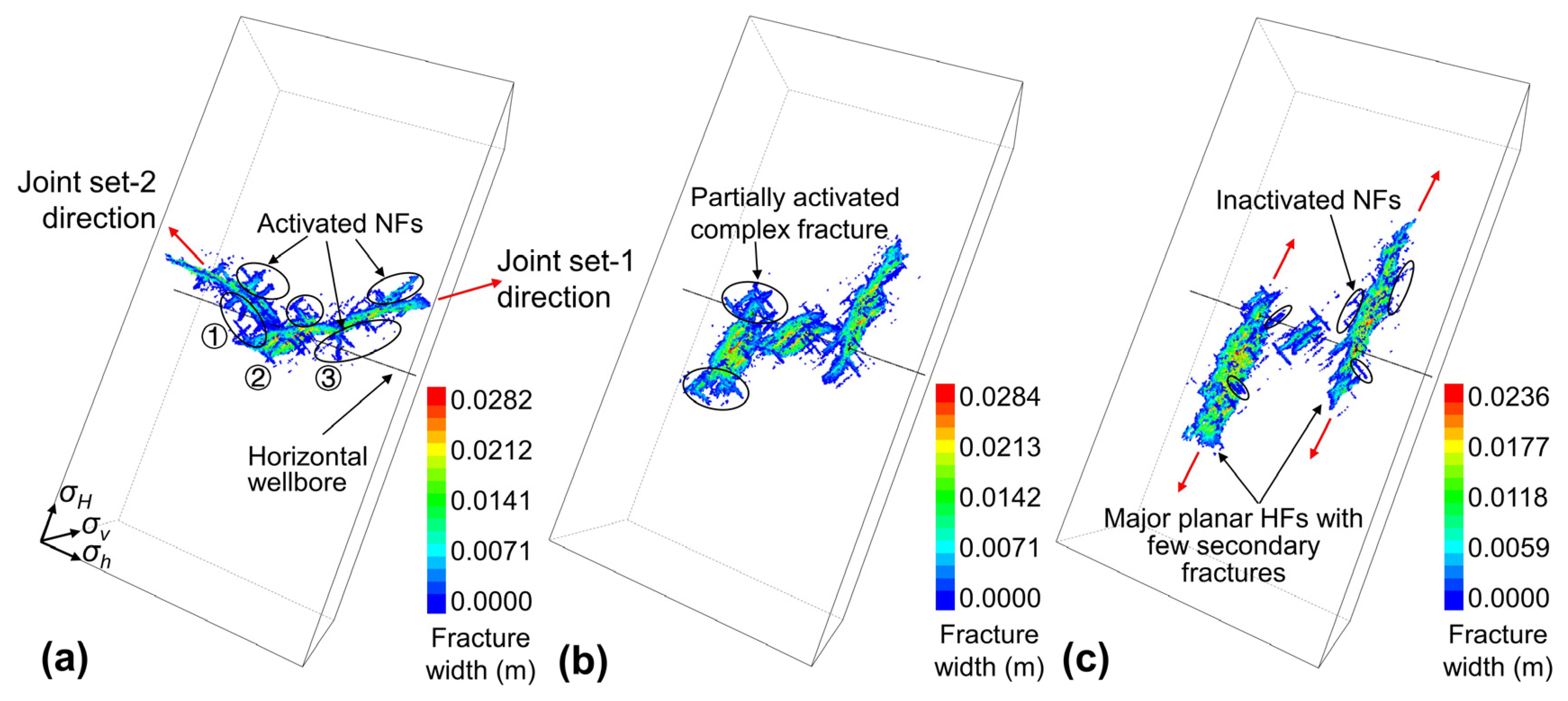
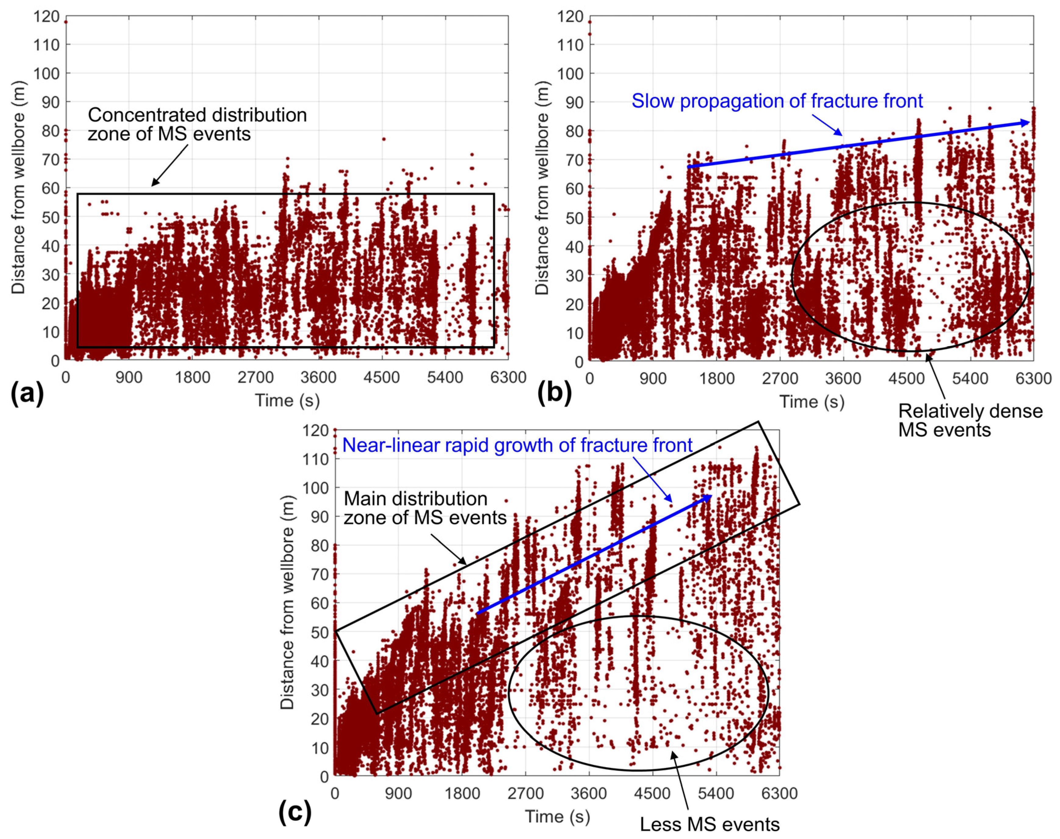
4.1. Injection Rate

Injection rates of 11 m³/min, 13 m³/min, and 17 m³/min are run to understand its impact on fracture propagation, and the results are shown in Figure 7. It is noted that the same fluid volume for different cases is applied.

Figure 7 illustrates that with the increase of injection rate, the main hydraulic fracture in the second cluster gradually propagates further and activates more natural fractures, thus resulting in the relatively balanced propagation of three-cluster fractures. This means that a high injection rate is able to overcome the stress shadow effect of the outermost clusters (the first and the third clusters) on the middle cluster. Additionally, more natural fractures are reactivated at high injection rates, thereby forming a secondary fracture network (Figure 7c). Moreover, when the injection rate increases from 11 m³/min to 17 m³/min, the fracture width of hydraulic fractures gradually increases from 0.0265 m to 0.0292 m, a 10.19% increment.

With a high injection rate of 17 m³/min, more microseismic events are generated, and these microseismic events are densely distributed in the affected region of hydraulic fractures (Figure 8c). Even in the later stage of fracturing, there are still a large number of microseismic events generated in the far-field, implying that a high injection rate is able to stimulate the majority of the target reservoir. In contrast, microseismic events under the low injection rate are mainly concentrated in the near-wellbore area in the early stage of fracturing, while few microseismic events are scattered and unevenly distributed in the far-field in the later stage of fracturing, indicating that a low injection rate is not able to stimulate the far-field. This is because it is difficult for fracturing fluid to fill the newly created fracture promptly in the far-field and the filtration of fracturing fluid when the injection rate is low.

As the injection rate increases from 11 m³/min to 17 m³/min, the total volume of hydraulic fractures increases linearly by 24.93% (42.63 m³), as shown in Figure 9a. In addition, with the increment of injection rate, the proportion of fracture volume of the outermost clusters (the first and third clusters) gradually decreases, whereas the proportion of fracture volume of the second cluster gradually increases. This results in a change in the fracture volume ratio of the three clusters from the initial 0.44:0.08:0.48 (standard deviation of 0.18) to 0.32:0.29:0.39 (standard deviation of 0.04), showing that the high injection rate significantly improves the even propagation of multi-cluster fractures. It is noted that the total volume of hydraulic fractures is approximately 12~16% of the total injected fluid, this is because the high leakoff of fracturing fluid in fractured shale reservoirs (with a leakoff coefficient of 2 × 10⁻⁴ m/s^0.5) causes a large amount of fluid filtration into the natural fractures and rock matrix, resulting in a lower stimulation efficiency.

In summary, we can conclude that the high injection rate of fracturing fluid needs to be applied during hydraulic fracturing in fractured shale reservoirs. This not only allows for the creation of a complex fracture network to increase the total fracture volume, but also improves the uniform propagation of multi-cluster fractures. At the same time, a high injection rate can help the far-field stimulation in the reservoir. It is noted that a high injection rate might lead to frac-hits between adjacent horizontal wells. Therefore, the appropriate injection rate needs to be determined in combination with field experience or further research.

4.2. Horizontal Stress Difference

We ran simulation models with three different horizontal stress differences: 0 MPa, 5 MPa, and 10 MPa. The fracture morphologies are shown in Figure 10. When the two horizontal stresses are equal (Figure 10a), the main hydraulic fractures deflect after encountering natural fractures near the wellbore and then propagate along with the strike directions of two sets of conjugate joints. Specifically, the left-wing of the main hydraulic fractures mainly propagates along the strike direction of joint set-2, and the right-wing propagates along the strike direction of joint set-1. The formation of the main fracture almost parallel to the horizontal wellbore leads to the connection of three clusters near-wellbore. In addition, secondary fractures with different strike directions connected by the main hydraulic fracture are completely activated. As can be seen from Figure 10b,c, hydraulic fractures tend to directly cross natural fractures to form major transverse fractures propagating along the optimal direction under a high horizontal stress difference. With the increase of horizontal stress difference, natural fractures intersected by hydraulic fractures are difficult to be activated, resulting in a simple fracture morphology, such as the main planar fractures with few secondary fractures, as shown in Figure 10c. Moreover, due to the large horizontal stress difference, the fracture propagation of the middle cluster becomes suppressed. This is because the formation of the outermost fractures has significant stress interference on the middle cluster, which inhibits the propagation of the middle fracture if the horizontal stress difference is too large.

Microseismic events during the fracturing process are mainly concentrated within 60 m of the wellbore when there are no horizontal stress differences (Figure 11a). As injection time increases, microseismic events do not occur in the far-field, indicating that hydraulic fractures do not propagate far into the formation. This is consistent with the phenomenon shown in Figure 10a, i.e., the main hydraulic fracture propagates parallel to the wellbore direction due to the influence of pre-existing natural fractures.

With a horizontal stress difference of 5 MPa, microseismic events gradually appear in the far-field as injection time increases from 1389 s to 6300 s (Figure 11b), which indicates that the front of hydraulic fractures slowly propagates forward. In addition, relatively dense microseismic events are still generated near the wellbore in the later stage of fracturing (black ellipse in Figure 11b), implying that a large amount of fracturing fluid is consumed by reservoir stimulation in the near-wellbore area, with the adverse effect of reducing fracturing fluid volume used for far-field stimulation.

As the horizontal stress difference is increased to 10 MPa, microseismic events are concentrated in the black rectangular box in Figure 11c, whereas microseismic events outside the rectangular box are relatively rare and sparse, especially near-wellbore in the later stage of fracturing (black ellipse in Figure 11c). The overall distribution of microseismic events shows that the distance of microseismic events increases almost linearly with time, implying that hydraulic fractures propagate rapidly toward the far-field. Moreover, microseismic events are rarely generated near the wellbore in the later stage of fracturing, indicating that less fracturing fluid is consumed near-wellbore and indirectly implying that hydraulic fractures near the wellbore are relatively simple in geometry. These are beneficial to the far-field stimulation, which is consistent with the simulation results shown in Figure 10c.

Figure 12 shows that, as the horizontal stress difference increases from 0 MPa to 10 MPa, the total fracture volume is gradually reduced by 11.28% (22.20 m³). This is because natural fractures are prone to be activated to form a complex fracture network under a low horizontal stress difference, which significantly improves the stimulation effect. In addition, the fracture volume ratio of the three clusters is changed from 0.35:0.33:0.32 to 0.48:0.03:0.49 as the horizontal stress difference increases, and the corresponding standard deviation is increased from 0.01 to 0.21, indicating a reduction in uniform propagation of multi-cluster fractures. From this point of view, selecting the landing location of a horizontal wellbore with a low horizontal stress difference as a fracturing sweet spot is helpful to improve the stimulation effect.

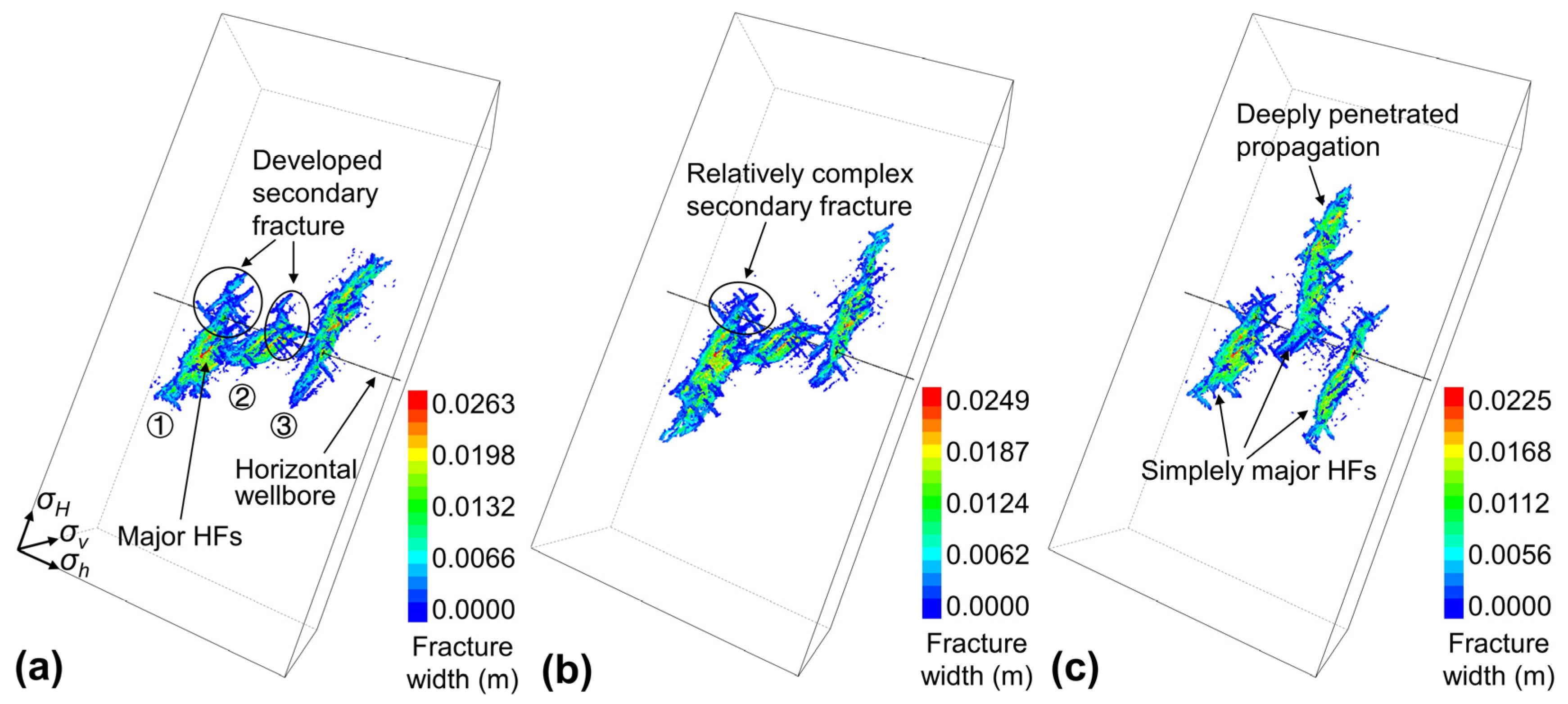
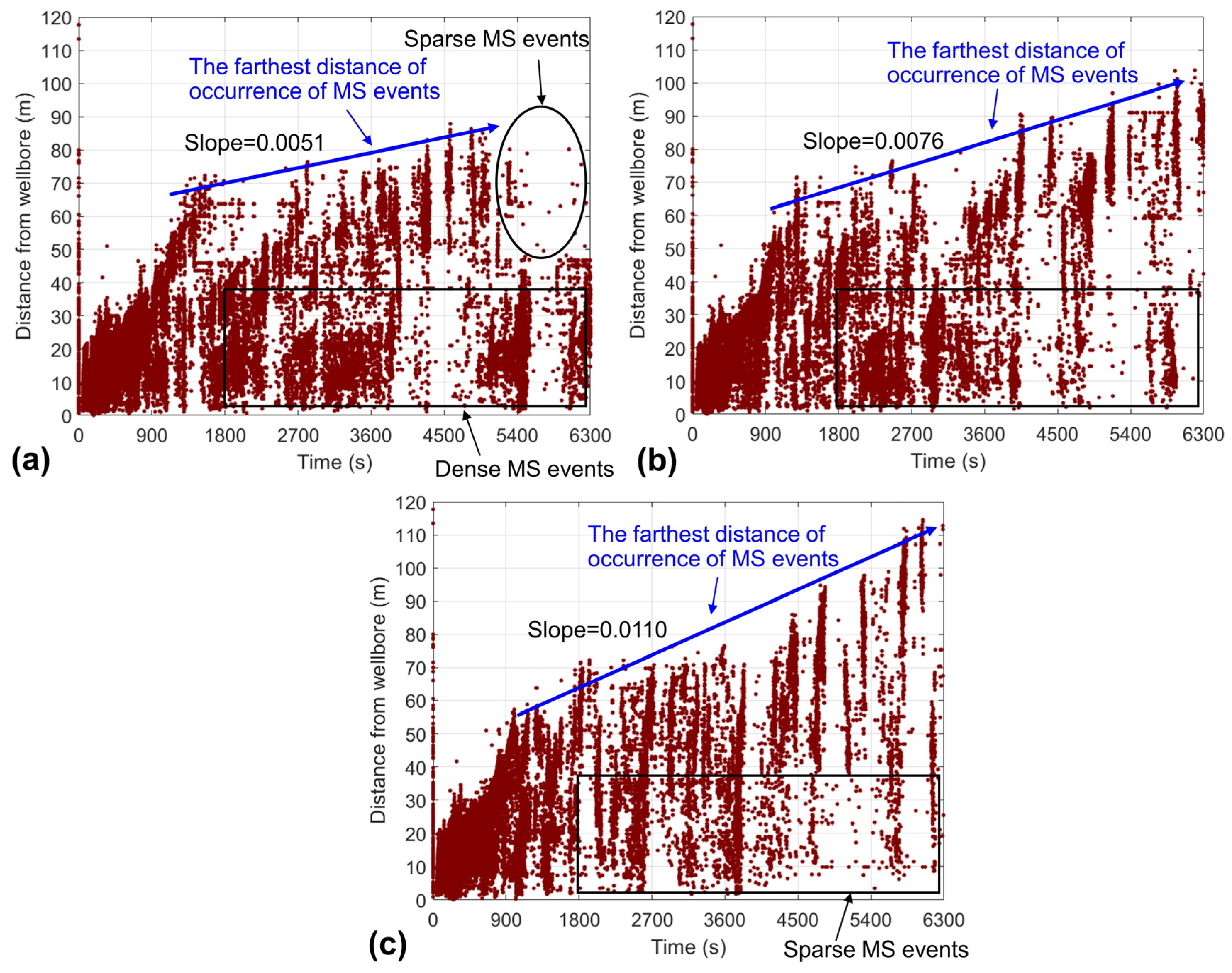
4.3. Fluid Viscosity

Figure 13 shows the fracture morphologies with fluid viscosities of 1 mPa.s, 30 mPa.s, and 120 mPa.s, respectively.

With a low fluid viscosity of 1 mPa.s, it is easy for the main hydraulic fractures to open or shear natural fractures, resulting in a developed secondary fracture network (Figure 13a). As the fluid viscosity increases, main hydraulic fractures extend further, while the complexity of the activated secondary fracture network is reduced, resulting in a simpler fracture network. In addition, the interaction of natural fractures with the main fracture in the second cluster is gradually reduced, resulting in this main fracture crossing the natural fracture directly and then propagating perpendicular to the direction of the minimum horizontal stress to the far-field. Ultimately, simple main fractures with undeveloped secondary fractures are generated from all three clusters, as shown in Figure 13c.

As the fracturing time increases, the maximum distance at which microseismic events occur increases gradually with a slope of 0.0051 when the fluid viscosity is 1 mPa.s (Figure 14a). In the later stage of fracturing (5400~6300 s), microseismic events are rarely generated in the far-field (black ellipse in Figure 14a) and are mainly concentrated near the wellbore. This is because hydraulic fractures under low fluid viscosity are easy to rotate and propagate along and activate natural fractures near the wellbore. When excessive natural fractures are opened or sheared near the wellbore, almost all fracturing fluid is consumed to create complex fracture networks and the high leakoff near the wellbore results in a small amount of fracturing fluid available for far-field stimulation. Therefore, there are fewer microseismic events in the far-field, reducing stimulation efficiency. In addition, with increasing injection time, the farthest distance where microseismic events occur gradually increases with increased slopes of 0.0051, 0.0076, and 0.0110, respectively. The corresponding growth rates of the slopes are 49.02% and 44.74%, respectively. These results show that the high injection rate significantly promotes the rapid propagation of hydraulic fractures into the far-field. Furthermore, the distribution of microseismic events near the wellbore with different viscosities, as shown in the black rectangular box in Figure 14, demonstrates that the higher the fluid viscosity, the fewer the microseismic events near the wellbore in the later stage of fracturing (1800~6300 s). According to the analysis, hydraulic fractures under the high viscosity fracturing fluid often cross natural fractures directly near the wellbore to the far-field.

In summary, hydraulic fractures can be easily affected by natural fractures under low fluid viscosity, which causes the activation of natural fractures and the formation of a complex fracture network. Consequently, the propagation of hydraulic fractures is limited. However, hydraulic fractures under high viscosity fluid are prone to cross natural fractures directly, resulting in the creation of simple hydraulic fractures. Therefore, for areas with dense natural fractures near the wellbore, it is recommended to use high viscosity fracturing fluid in the initial stage of fracturing to allow simple hydraulic fractures to directly cross natural fractures near the wellbore, thus avoiding the limited propagation of hydraulic fractures. Then, low viscosity fracturing fluid is used to maximize the activation of natural fractures in the far-field, thus forming a complex fracture network to effectively stimulate the reservoir.

5. Discussion

In this work, a randomly generated complex discrete fracture network is successfully added to the fracturing numerical model, and a three-dimensional field-scale model of the hydraulic fracture network is established. Different from previous studies in which the scale of natural fractures is equivalent to or even larger than that of hydraulic fractures [45,46,47], our model investigates the complex propagation of a fracture network when a large number of small-scale natural fractures (compared with hydraulic fractures) are present in fractured shale reservoir. Our simulation results show that when the dimension of natural fractures {(2~8 m) × (6~24 m)} is much smaller than that of hydraulic fractures {(70~90 m) × (90~150 m)}, the hydraulic fracture morphology is usually “main hydraulic fractures + complex secondary fractures”, which is different from that of the complex fracture network without main hydraulic fractures formed when the scales of natural fractures and hydraulic fractures are similar [48,49,50,51,52]. In our simulation, the propagation of the main hydraulic fractures is primarily controlled by in situ stresses, and the optimal propagation direction is perpendicular to the direction of the minimum horizontal stress. When a large-scale hydraulic fracture encounters a small-scale natural fracture, even if it is arrested and then offsets and propagates along the natural fracture and forms a secondary branched fracture due to either geological conditions or engineering operations, it only affects the local propagation and does not affect the overall propagation of the fracture network.

6. Conclusions

In this work, we established a three-dimensional numerical model for hydraulic fracturing with thousands of natural fractures in fractured shale reservoirs. Subsequently, we explored the propagation behaviors of complex fracture networks under the influence of injection rate, horizontal stress difference, and fluid viscosity in detail. The following conclusions can be drawn.

(1) The fracture morphology of “main hydraulic fractures + complex secondary fractures” is usually formed in fractured shale reservoirs when the scale of hydraulic fractures is much larger than that of natural fractures.

(2) The spatial growth and evolution of the fracture network can be reflected by the evolution of microseismic events during the numerical simulation.

(3) As the injection rate increases from 11 m³/min to 17 m³/min, the total fracture volume increases nearly linearly with an increment of 24.93% (42.63 m³), and the standard deviation of fracture volume ratio of three clusters decreases from 0.18 to 0.04, indicating a significant improvement in the uniform propagation of multi-cluster fractures. Therefore, a high injection rate is recommended for hydraulic fracturing in the field.

(4) As the horizontal stress difference increases from 0 MPa to 10 MPa, the total fracture volume is reduced by 11.28%, and the standard deviation of fracture volume ratio of three clusters increases from 0.01 to 0.21, indicating a significant reduction in the uniform stimulation of multi-cluster fractures. Therefore, landing the horizontal wellbore in a zone with a low horizontal stress difference can help improve the stimulation efficiency.

(5) For zones with a large number of natural fractures near the wellbore, it is recommended to use high viscosity fracturing fluid (e.g., 120 mPa.s) in the initial stage of fracturing to allow simple hydraulic fractures to directly cross natural fractures near the wellbore, thus avoiding the limited propagation of hydraulic fractures. Low viscosity fracturing fluid (e.g., 1 mPa.s) is then used to activate the far-field natural fractures, thereby maximizing fracture complexity and improving stimulation efficiency.

References

1. Wang, D.-J.; Tang, H.; Shen, P.; Su, X.; Huang, L. Co-effects of bedding planes and parallel flaws on fracture evolution in anisotropic rocks. Eng. Geol. 2020, 264, 105382. [Google Scholar] [CrossRef]
2. Elizalde, C.; Griffith, W.A.; Miller, T. Thrust fault nucleation due to heterogeneous bedding plane slip: Evidence from an Ohio coal mine. Eng. Geol. 2016, 206, 1–17. [Google Scholar] [CrossRef]
3. Ma, G.; Li, M.; Wang, H.; Chen, Y. Equivalent discrete fracture network method for numerical estimation of deformability in complexly fractured rock masses. Eng. Geol. 2020, 277, 105784. [Google Scholar] [CrossRef]
4. Zhao, H.; Wang, X.; Liu, Z. Experimental investigation of hydraulic sand fracturing on fracture propagation under the influence of coal macrolithotypes in Hancheng block, China. J. Pet. Sci. Eng. 2019, 175, 60–71. [Google Scholar] [CrossRef]
5. Tang, J.; Wu, K.; Zuo, L.; Xiao, L.; Sun, S.; Ehlig–Economides, C. Investigation of rupture and slip mechanisms of hydraulic fracture in multiple-layered formation. SPE J. 2019, 24, 2292–2307. [Google Scholar] [CrossRef]
6. Xie, J.; Tang, J.; Yong, R.; Fan, Y.; Zuo, L.; Chen, X.; Li, Y. A 3-D hydraulic fracture propagation model applied for shale gas reservoirs with multiple bedding planes. Eng. Fract. Mech. 2020, 228, 106872. [Google Scholar] [CrossRef]
7. Tan, P.; Jin, Y.; Pang, H. Hydraulic fracture vertical propagation behavior in transversely isotropic layered shale formation with transition zone using XFEM-based CZM method. Eng. Fract. Mech. 2021, 248, 107707. [Google Scholar] [CrossRef]
8. Haddad, M.; Du, J.; Vidal-Gilbert, S. Integration of dynamic microseismic data with a true 3d modeling of hydraulic-fracture propagation in the Vaca Muerta shale. SPE J. 2017, 22, 1714–1738. [Google Scholar] [CrossRef]
9. Mejía Camones, L.A.; Vargas, E.d.A.; Velloso, R.Q.; Paulino, G.H. Simulation of hydraulic fracturing processes in rocks by coupling the lattice Boltzmann model and the Park-Paulino-Roesler potential-based cohesive zone model. Int. J. Rock Mech. Min. Sci. 2018, 112, 339–353. [Google Scholar] [CrossRef]
10. Ouchi, H.; Katiyar, A.; Foster, J.T.; Sharma, M.M. A peridynamics model for the propagation of hydraulic fractures in naturally fractured reservoirs. SPE J. 2017, 22, 1082–1102. [Google Scholar] [CrossRef]
11. Tan, P.; Pang, H.; Zhang, R.; Jin, Y.; Zhou, Y.; Kao, J.; Fan, M. Experimental investigation into hydraulic fracture geometry and proppant migration characteristics for southeastern Sichuan deep shale reservoirs. J. Pet. Sci. Eng. 2020, 184, 106517. [Google Scholar] [CrossRef]
12. Li, M.; Zhang, F.; Zhuang, L.; Zhang, X.; Ranjith, P. Micromechanical analysis of hydraulic fracturing in the toughness-dominated regime: Implications to supercritical carbon dioxide fracturing. Comput. Geosci. 2020, 24, 1815–1831. [Google Scholar] [CrossRef]
13. Maity, D.; Ciezobka, J. Digital fracture characterization at hydraulic fracturing test site hfts-midland: Fracture clustering, stress effects and lithologic controls. In Proceedings of the SPE Hydraulic Fracturing Technology Conference and Exhibition, Virtual, 4–6 May 2021. [Google Scholar]
14. Ru, Z.; Hu, J.; Madni, A.S.; An, K. A study on the optimal conditions for formation of complex fracture networks in fractured reservoirs. J. Struct. Geol. 2020, 135, 104039. [Google Scholar] [CrossRef]
15. Guo, Z.; Tian, S.; Liu, Q.; Ma, L.; Yong, Y.; Yang, R. Experimental investigation on the breakdown pressure and fracture propagation of radial borehole fracturing. J. Pet. Sci. Eng. 2022, 208, 109169. [Google Scholar] [CrossRef]
16. Zhao, H.; Wang, X.; Liu, Z.; Yan, Y.; Yang, H. Investigation on the hydraulic fracture propagation of multilayers-commingled fracturing in coal measures. J. Pet. Sci. Eng. 2018, 167, 774–784. [Google Scholar] [CrossRef]
17. Yang, B.; Wang, H.; Wang, B.; Shen, Z.; Zheng, Y.; Jia, Z.; Yan, W. Digital quantification of fracture in full-scale rock using micro-CT images: A fracturing experiment with N2 and CO2. J. Pet. Sci. Eng. 2021, 196, 107682. [Google Scholar] [CrossRef]
18. Zhai, L.; Zhang, H.; Pan, D.; Zhu, Y.; Zhu, J.; Zhang, Y.; Chen, C. Optimisation of hydraulic fracturing parameters based on cohesive zone method in oil shale reservoir with random distribution of weak planes. J. Nat. Gas Sci. Eng. 2020, 75, 103130. [Google Scholar] [CrossRef]
19. Wang, H. Hydraulic fracture propagation in naturally fractured reservoirs: Complex fracture or fracture networks. J. Nat. Gas Sci. Eng. 2019, 68, 102911. [Google Scholar] [CrossRef] [Green Version]
20. Yu, H.; Dahi Taleghani, A.; Lian, Z. On how pumping hesitations may improve complexity of hydraulic fractures, a simulation study. Fuel 2019, 249, 294–308. [Google Scholar] [CrossRef]
21. Zou, J.; Jiao, Y.-Y.; Tan, F.; Lv, J.; Zhang, Q. Complex hydraulic-fracture-network propagation in a naturally fractured reservoir. Comput. Geotech. 2021, 135, 104165. [Google Scholar] [CrossRef]
22. Fan, H.; Li, S.; Feng, X.-T.; Zhu, X. A high-efficiency 3D boundary element method for estimating the stress/displacement field induced by complex fracture networks. J. Pet. Sci. Eng. 2020, 187, 106815. [Google Scholar] [CrossRef]
23. Ren, L.; Su, Y.; Zhan, S.; Hao, Y.; Meng, F.; Sheng, G. Modeling and simulation of complex fracture network propagation with SRV fracturing in unconventional shale reservoirs. J. Nat. Gas Sci. Eng. 2016, 28, 132–141. [Google Scholar] [CrossRef]
24. Cheng, W.; Wang, R.; Jiang, G.; Xie, J. Modelling hydraulic fracturing in a complex-fracture-network reservoir with the DDM and graph theory. J. Nat. Gas Sci. Eng. 2017, 47, 73–82. [Google Scholar] [CrossRef]
25. Shakiba, M.; de Araujo Cavalcante Filho, J.S.; Sepehrnoori, K. Using embedded discrete fracture model (EDFM) in numerical simulation of complex hydraulic fracture networks calibrated by microseismic monitoring data. J. Nat. Gas Sci. Eng. 2018, 55, 495–507. [Google Scholar] [CrossRef]
26. Li, J.; Yu, W.; Guerra, D.; Wu, K. Modeling wettability alteration effect on well performance in Permian basin with complex fracture networks. Fuel 2018, 224, 740–751. [Google Scholar] [CrossRef]
27. Shi, F.; Wang, X.; Liu, C.; Liu, H.; Wu, H. An XFEM-based method with reduction technique for modeling hydraulic fracture propagation in formations containing frictional natural fractures. Eng. Fract. Mech. 2017, 173, 64–90. [Google Scholar] [CrossRef]
28. Dong, Y.; Li, P.; Tian, W.; Xian, Y.; Lu, D. An equivalent method to assess the production performance of horizontal wells with complicated hydraulic fracture network in shale oil reservoirs. J. Nat. Gas Sci. Eng. 2019, 71, 102975. [Google Scholar] [CrossRef]
29. Qin, M.; Yang, D.; Chen, W.; Xia, X. Hydraulic fracturing network modeling based on peridynamics. Eng. Fract. Mech. 2021, 247, 107676. [Google Scholar] [CrossRef]
30. Zhang, J.; Li, Y.; Pan, Y.; Wang, X.; Yan, M.; Shi, X.; Zhou, X.; Li, H. Experiments and analysis on the influence of multiple closed cemented natural fractures on hydraulic fracture propagation in a tight sandstone reservoir. Eng. Geol. 2021, 281, 105981. [Google Scholar] [CrossRef]
31. Liu, Z.; Wang, S.; Zhao, H.; Wang, L.; Li, W.; Geng, Y.; Tao, S.; Zhang, G.; Chen, M. Effect of random natural fractures on hydraulic fracture propagation geometry in fractured carbonate rocks. Rock Mech. Rock Eng. 2018, 51, 491–511. [Google Scholar] [CrossRef]
32. Tan, P.; Jin, Y.; Han, K.; Hou, B.; Chen, M.; Guo, X.; Gao, J. Analysis of hydraulic fracture initiation and vertical propagation behavior in laminated shale formation. Fuel 2017, 206, 482–493. [Google Scholar] [CrossRef]
33. Damjanac, B.; Detournay, C.; Cundall, P.A. Application of particle and lattice codes to simulation of hydraulic fracturing. Comput. Part. Mech. 2016, 3, 249–261. [Google Scholar] [CrossRef]
34. Benouadah, N.; Djabelkhir, N.; Song, X.; Rasouli, V.; Damjanac, B. Simulation of competition between transverse notches versus axial fractures in open hole completion hydraulic fracturing. Rock Mech. Rock Eng. 2021, 54, 2249–2265. [Google Scholar] [CrossRef]
35. Bakhshi, E.; Rasouli, V.; Ghorbani, A.; Fatehi Marji, M.; Damjanac, B.; Wan, X. Lattice numerical simulations of lab-scale hydraulic fracture and natural interface interaction. Rock Mech. Rock Eng. 2019, 52, 1315–1337. [Google Scholar] [CrossRef]
36. Damjanac, B.; Cundall, P. Application of distinct element methods to simulation of hydraulic fracturing in naturally fractured reservoirs. Comput. Geotech. 2016, 71, 283–294. [Google Scholar] [CrossRef]
37. Zhang, F.; Wang, X.; Tang, M.; Du, X.; Xu, C.; Tang, J.; Damjanac, B. Numerical investigation on hydraulic fracturing of extreme limited entry perforating in plug-and-perforation completion of shale oil reservoir in Changqing oilfield, China. Rock Mech. Rock Eng. 2021, 54, 2925–2941. [Google Scholar] [CrossRef]
38. Zhang, F.; Wu, J.; Huang, H.; Wang, X.; Luo, H.; Yue, W.; Hou, B. Technological parameter optimization for improving the complexity of hydraulic fractures in deep shale reservoirs. Nat. Gas Ind. 2021, 41, 125–135. [Google Scholar] [CrossRef]
39. Wang, X.; Zhang, F.; Tang, M.; Du, X.; Tang, J. Effect of stress shadow caused by multi-stage fracturing from multiple well pads on fracture initiation and near-wellbore propagation from infill wells. SPE J. 2021, 1–22. [Google Scholar] [CrossRef]
40. Zhang, F.; Mack, M. Integrating fully coupled geomechanical modeling with microsesmicity for the analysis of refracturing treatment. J. Nat. Gas Sci. Eng. 2017, 46, 16–25. [Google Scholar] [CrossRef]
41. Zou, Y.; Ma, X.; Zhang, S.; Zhou, T.; Li, H. Numerical investigation into the influence of bedding plane on hydraulic fracture network propagation in shale formations. Rock Mech. Rock Eng. 2016, 49, 3597–3614. [Google Scholar] [CrossRef]
42. Heng, S.; Li, X.; Liu, X.; Chen, Y. Experimental study on the mechanical properties of bedding planes in shale. J. Nat. Gas Sci. Eng. 2020, 76, 103161. [Google Scholar] [CrossRef]
43. Nagel, N.B.; Garcia, X.; Sanchez Nagel, M.; Lee, B. Understanding “SRV”: A numerical investigation of “wet” vs. “dry” microseismicity during hydraulic fracturing. In Proceedings of the SPE Annual Technical Conference and Exhibition, San Antonio, TX, USA, 8–10 October 2012. [Google Scholar]
44. Maxwell, S.C.; Mack, M.; Zhang, F.; Chorney, D.; Goodfellow, S.D.; Grob, M. Differentiating wet and dry microseismic events induced during hydraulic fracturing. In Proceedings of the Unconventional Resources Technology Conference, San Antonio, TX, USA, 20–22 July 2015. [Google Scholar]
45. Li, S.; Zhang, D.; Li, X. A new approach to the modeling of hydraulic-fracturing treatments in naturally fractured reservoirs. SPE J. 2017, 22, 1064–1081. [Google Scholar] [CrossRef]
46. Zou, Y.; Zhang, S.; Ma, X.; Zhou, T.; Zeng, B. Numerical investigation of hydraulic fracture network propagation in naturally fractured shale formations. J. Struct. Geol. 2016, 84, 1–13. [Google Scholar] [CrossRef]
47. Maxwell, S.C.; Zhang, F.; Damjanac, B. Geomechanical modeling of induced seismicity resulting from hydraulic fracturing. Lead. Edge 2015, 34, 678–683. [Google Scholar] [CrossRef] [Green Version]
48. Kresse, O.; Weng, X.; Chuprakov, D.; Prioul, R.; Cohen, C. Effect of flow rate and viscosity on complex fracture development in UFM model. In Proceedings of the ISRM International Conference for Effective and Sustainable Hydraulic Fracturing, Brisbane, Australia, 20–22 May 2013. [Google Scholar]
49. Zhao, H.; Wang, X.; Wang, W.; Mu, E. A simulation method based on energy criterion for network fracturing in shale gas reservoirs. J. Nat. Gas Sci. Eng. 2018, 52, 295–303. [Google Scholar] [CrossRef]
50. Meyer, B.R.; Bazan, L.W. A discrete fracture network model for hydraulically induced fractures: Theory, parametric and case studies. In Proceedings of the SPE Hydraulic Fracturing Technology Conference, The Woodlands, TX, USA, 24–26 January 2011. [Google Scholar]
51. Li, S.; Zhang, D. How effective is carbon dioxide as an alternative fracturing fluid? SPE J. 2019, 24, 857–876. [Google Scholar] [CrossRef]
52. Ni, L.; Zhang, X.; Zou, L.; Huang, J. Phase-field modeling of hydraulic fracture network propagation in poroelastic rocks. Comput. Geosci. 2020, 24, 1767–1782. [Google Scholar] [CrossRef] [Green Version]
Figure 1. Discrete lattice method [39].
Energies 14 08297 g001
Figure 2. Three-dimensional numerical model of hydraulic fracturing with the discrete fracture network.
Energies 14 08297 g002
Figure 3. Three-dimensional discrete fracture network. (a) Top view, and (b) side view.
Energies 14 08297 g003
Figure 4. Fracturing simulation results. (a) Fracture morphologies, and (b) the distribution of microseismic events. The red bold arrow in figure (a) indicates the propagation direction of the main fractures. MS stands for microseismic.
Energies 14 08297 g004
Figure 5. The time vs. distance from the horizontal wellbore relationship of microseismic events. MS stands for microseismic.
Energies 14 08297 g005
Figure 6. The comparison of injection pressures between numerical simulation and field fracturing.
Energies 14 08297 g006
Figure 7. Fracture morphologies under different injection rates of (a) 11 m3/min, (b) 13 m3/min, and (c) 17 m3/min.
Energies 14 08297 g007
Figure 8. The time vs. distance relationship of microseismic events under different injection rates of (a) 11 m3/min, (b) 13 m3/min, and (c) 17 m3/min. MS stands for microseismic.
Energies 14 08297 g008
Figure 9. (a) The total volume of hydraulic fractures, and (b) the proportion of individual fracture volume under different injection rates.
Energies 14 08297 g009
Figure 10. Fracture morphologies under different horizontal stress differences of (a) 0 MPa, (b) 5 MPa, and (c) 10 MPa. The red arrow represents the propagation directions of the main fractures.
Energies 14 08297 g010
Figure 11. The time vs. distance relationship of microseismic events under different horizontal stress differences of (a) 0 MPa, (b) 5 MPa, and (c) 10 MPa. MS stands for microseismic.
Energies 14 08297 g011
Figure 12. (a) Total hydraulic fracture volume, and (b) the proportion of individual fracture volume under different horizontal stress differences.
Energies 14 08297 g012
Figure 13. Fracture morphologies under different fluid viscosities of (a) 1 mPa.s, (b) 30 mPa.s, and (c) 120 mPa.s.
Energies 14 08297 g013
Figure 14. The time vs. distance relationship of microseismic events under different fluid viscosities of (a) 1 mPa.s, (b) 30 mPa.s, and (c) 120 mPa.s. MS stands for microseismic.
Energies 14 08297 g014
Publisher’s Note: MDPI stays neutral with regard to jurisdictional claims in published maps and institutional affiliations.