
Three-Dimensional LiDAR Wake Measurements in an Offshore Wind Farm and Comparison with Gaussian and AL Wake Models


Abstract
:1. Introduction
2. Research Methodology
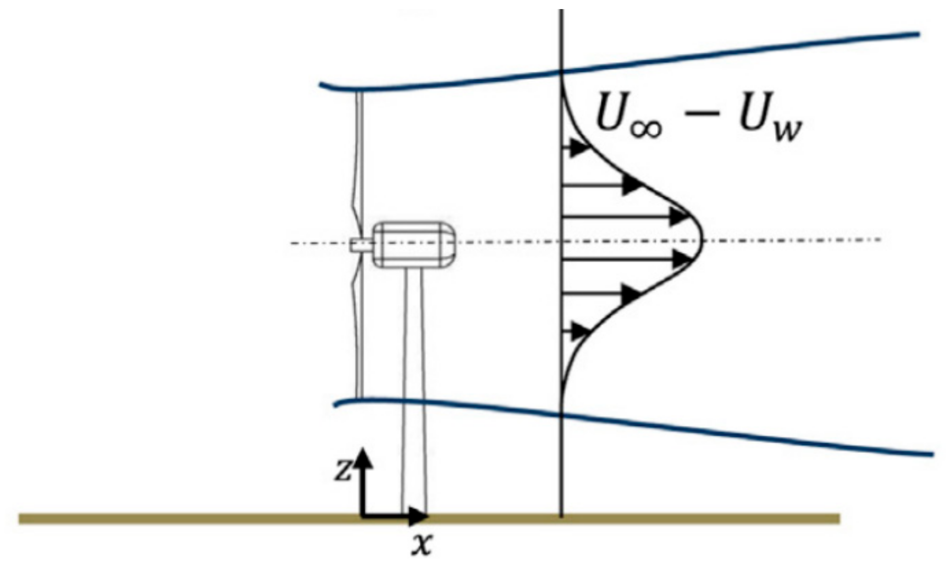
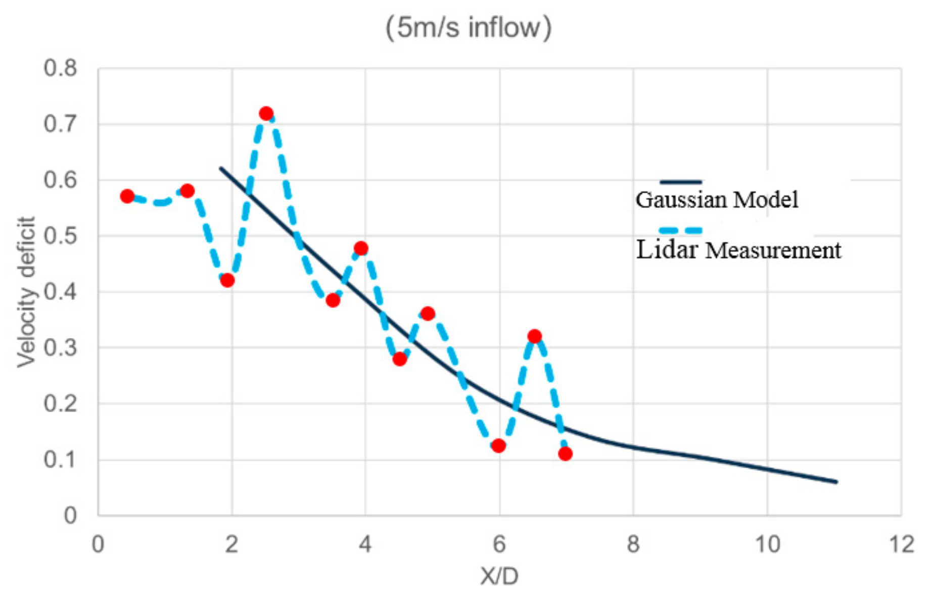
2.1. Gaussian Wake Model
- (1)
- The initial radius of the wake equals the rotor radius;
- (2)
- The velocity distribution in the wake area is nonlinear;
- (3)
- The velocity at any specific x distance in the downstream has a Gaussian distribution.
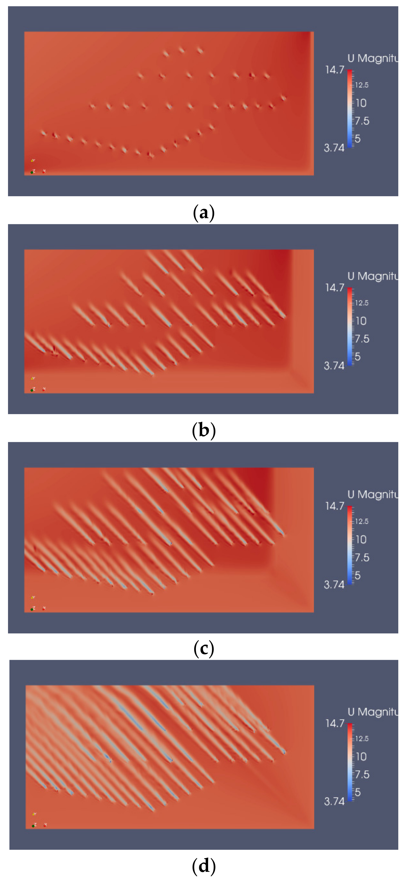
2.2. The Actuator Line Methods
3. Experiment
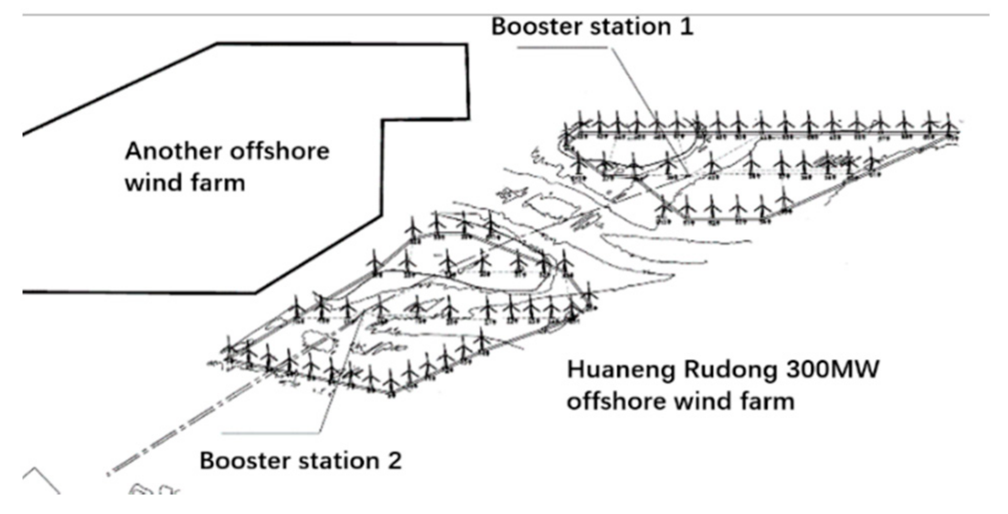
3.1. Wind Farm
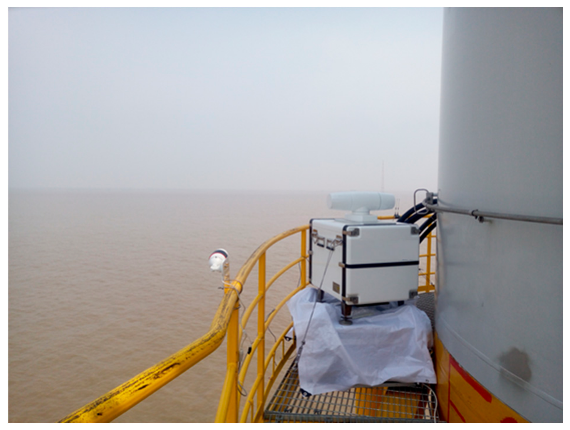
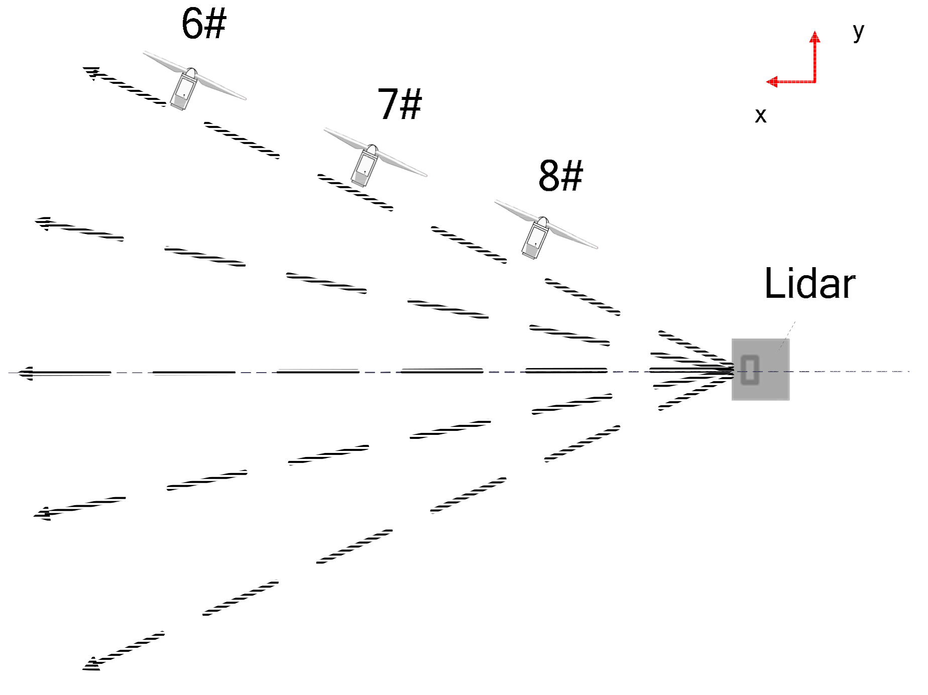
3.2. Experiment Setup
3.3. Lidar Data Processing
4. Results
5. Discussions
- (1)
- It takes some time for the wake to develop, and there is little impact on laterally area out of the wake at the beginning;
- (2)
- The diffusion velocity of the wake equals to the velocity of background wind;
- (3)
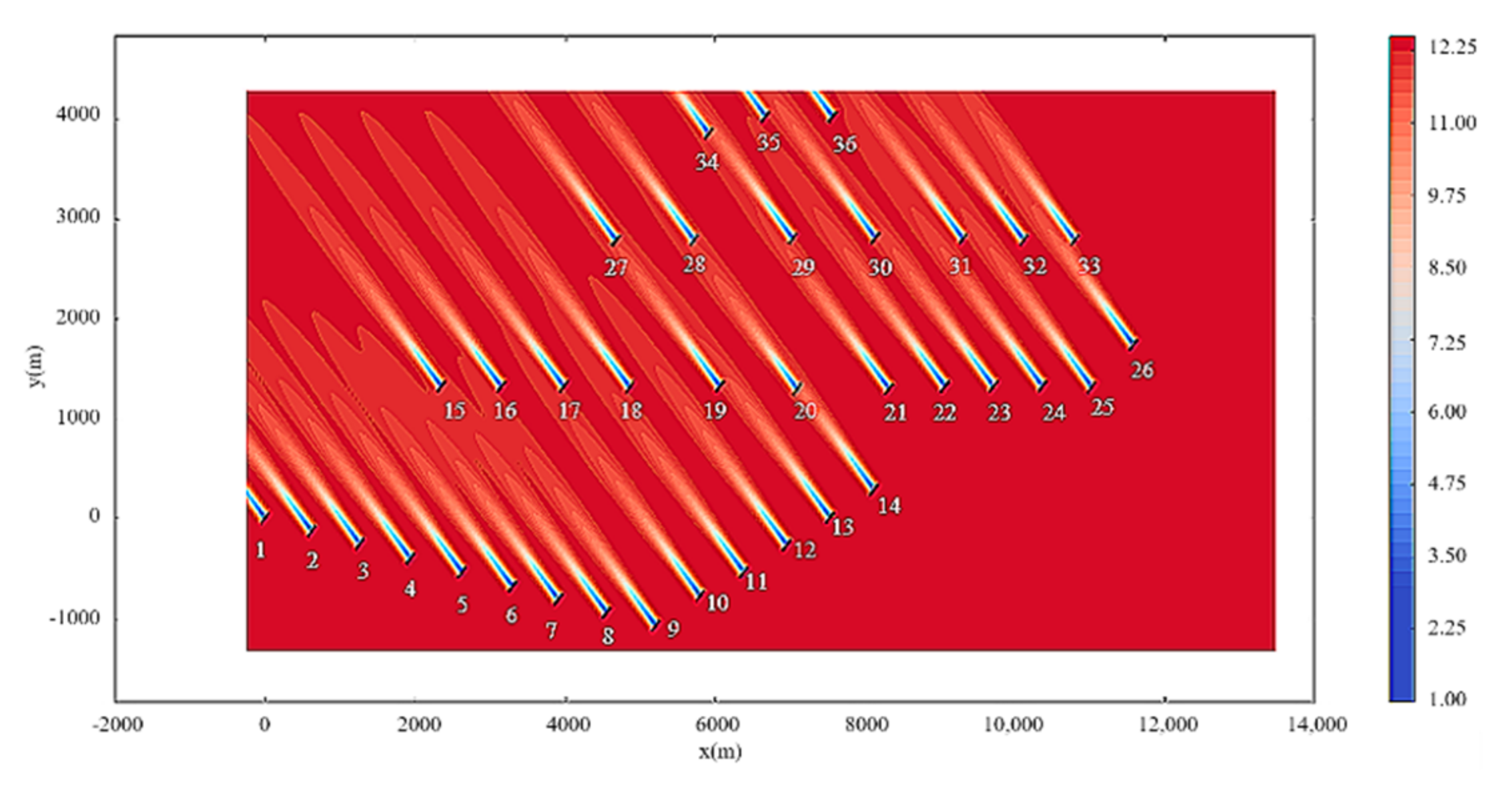
- In the dynamic view, the wake has volatility, and will not develop into a straight line even on flat terrain;
- (4)
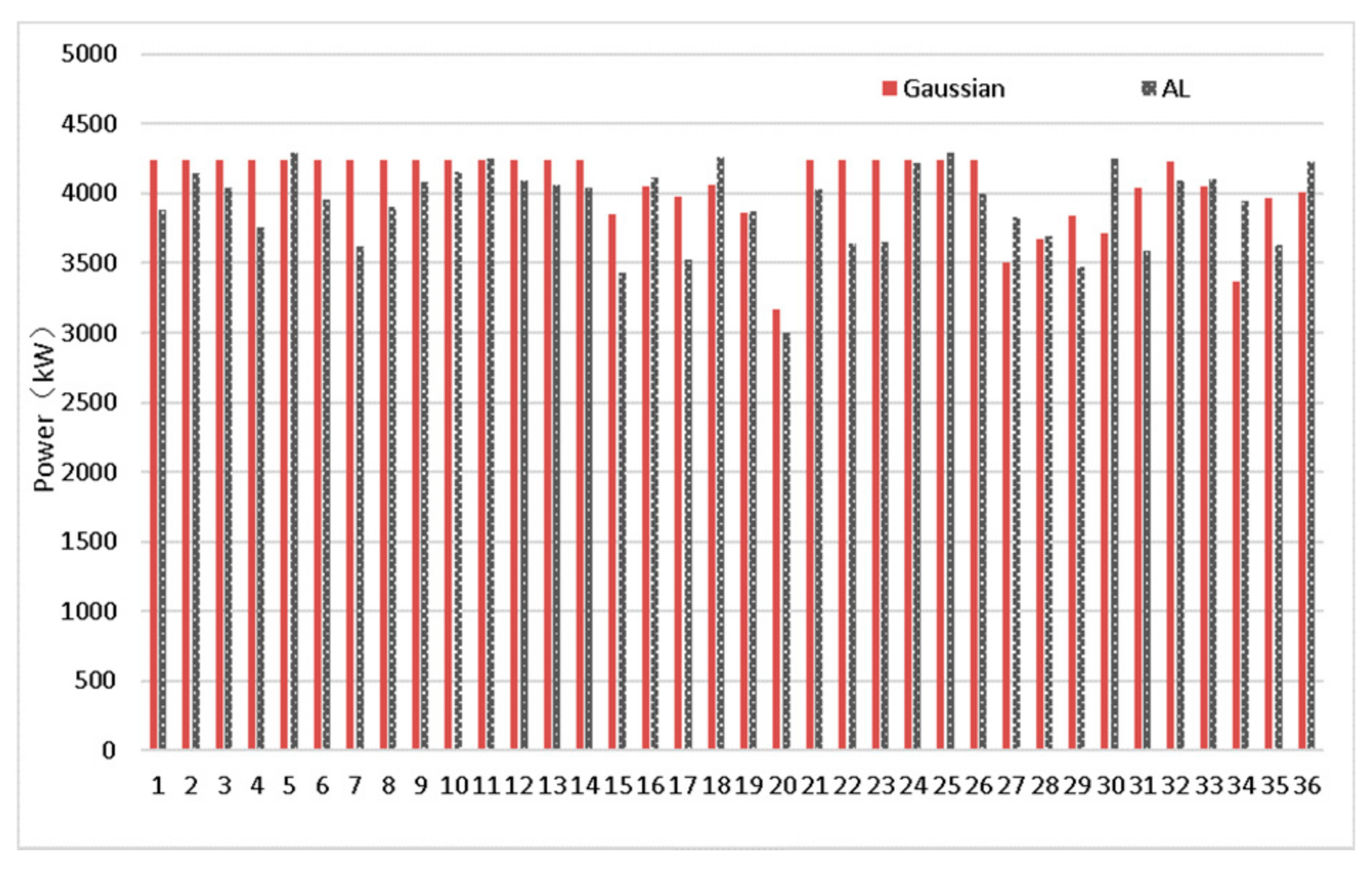
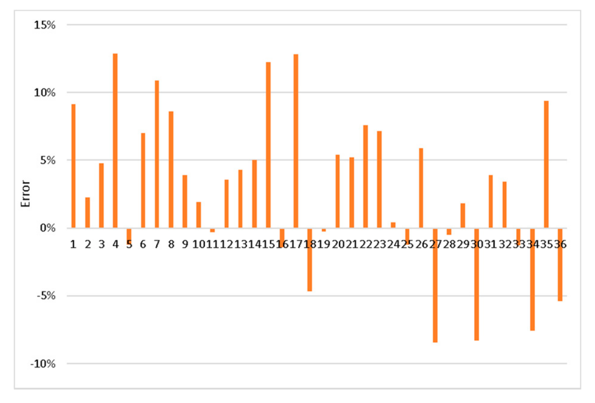
- The volatility of the wake causes the variance of power output;
- (5)
- The average characteristics of the volatility can be approximately analyzed by steady-state wake models.
6. Conclusions
Author Contributions
Funding
Informed Consent Statement
Conflicts of Interest
References
- Bitar, E.; Seiler, P. Coordinated control of a wind turbine array for power maximization. In Proceedings of the 2013 American Control Conference, Washington, DC, USA, 17–19 June 2013; pp. 2898–2904. [Google Scholar]
- Johnson, K.E.; Fritsch, G. Assessment of Extremum Seeking Control for Wind Farm Energy Production. Wind. Eng. 2012, 36, 701–715. [Google Scholar] [CrossRef]
- Johnson, K.E.; Thomas, N. Wind farm control: Addressing the aerodynamic interaction among wind turbines. In Proceedings of the 2009 American Control Conference, St. Louis, MO, USA, 10–12 June 2009; pp. 2104–2109. [Google Scholar]
- Schepers, J.G.; Van der Pijl, S.P. Improved modelling of wake aerodynamics and assessment of new farm control strategies. In Proceedings of the Science of Making Torque from Wind, Lyngby, Denmark, 28–31 August 2007; pp. 012039–012046. [Google Scholar]
- Smith, G.; Schlez, W.; Liddell, A.; Neubert, A.; Pena, A. Advanced wake model for very closely spaced turbines. In Proceedings of the European Wind Energy Conference 2006, Athens, Greece, 27 February–2 March 2006. [Google Scholar]
- Barber, S.; Chokani, N.; Abhari, R.S. Wind turbine performance and aerodynamics in wakes within wind farms. In Proceedings of the European Wind Energy Conference and Exhibition 2011, Brussels, Belgium, 14–17 March 2011. [Google Scholar]
- Ainslie, J. Calculating the flowfield in the wake of wind turbines. J. Wind. Eng. Ind. Aerodyn. 1988, 27, 213–224. [Google Scholar] [CrossRef]
- Sørensen, J.N.; Myken, A. Unsteady actuator disc model for horizontal axis wind turbines. J. Wind. Eng. Ind. Aerodyn. 1992, 39, 139–149. [Google Scholar] [CrossRef]
- Torres, P.; Van Wingerden, J.-W.; Verhaegen, M. Modeling of the flow in wind farms for total power optimization. In Proceedings of the 2011 9th IEEE International Conference on Control and Automation (ICCA), Santiago, Chile, 19–21 December 2011; pp. 963–968. [Google Scholar]
- Sørensen, N.; Johansen, J. UpWind: Aerodynamics and aero-elasticity Rotor aerodynamics in atmospheric shear flow. In Proceedings of the European Wind Energy Conference & Exhibition, EWEC 2007, Milan, Italy, 7–10 May 2007. [Google Scholar]
- Yang, X.; Sotiropoulos, F. On the predictive capabilities of LES-actuator disk model in simulating turbulence past wind turbines and farms. In Proceedings of the 2013 American Control Conference, Washington, DC, USA, 17–19 June 2013; pp. 2878–2883. [Google Scholar]
- Jensen, N.O. A Note on Wind Generator Interaction; Risø: Roskilde, Denmark, 1983. [Google Scholar]
- Parada, L.; Herrera, C.; Flores, P.; Parada, V. Wind farm layout optimization using a Gaussian-based wake model. Renew. Energy 2017, 107, 531–541. [Google Scholar] [CrossRef]
- Bastankhah, M.; Porté-Agel, F. A new analytical model for wind-turbine wakes. Renew. Energy 2014, 70, 116–123. [Google Scholar] [CrossRef]
- Bastankhah, M.; Porté-Agel, F. Experimental and theoretical study of wind turbine wakes in yawed conditions. J. Fluid Mech. 2016, 806, 506–541. [Google Scholar] [CrossRef]
- Niayifar, A.; Porté-Agel, F. A new analytical model for wind farm power prediction. J. Phys. Conf. Ser. 2015, 625, 012039. [Google Scholar] [CrossRef]
- Jha, P.; Churchfield, M.; Moriarty, P. Accuracy of state-of-the-art actuator-line modeling for wind turbine wakes. In Proceedings of the 51st AIAA Aerospace Sciences Meeting including the New Horizons Forum and Aerospace Exposition, Grapevine, TX, USA, 7–10 January 2013; p. 608. [Google Scholar]
- Hamlaoui, M.N.; Smaili, A.; Dobrev, I.; Pereira, M.; Fellouah, H.; Khelladi, S. Numerical and experimental investigations of HAWT near wake predictions using Particle Image Velocimetry and Actuator Disk Method. Energy 2022, 238, 121660. [Google Scholar] [CrossRef]
- Nilsson, K.; Shen, W.Z.; Sørensen, J.N.; Breton, S.P.; Ivanell, S. Validation of the actuator line method using near wake measurements of the MEXICO rotor. Wind. Energy 2015, 18, 499–514. [Google Scholar] [CrossRef]
- Kim, T.; Oh, S.; Yee, K. Improved actuator surface method for wind turbine application. Renew. Energy 2015, 76, 16–26. [Google Scholar] [CrossRef]
- Jin, J.; Hu, C. Stability analysis of offshore wind power monopile foundation under wind load. IOP Conf. Ser. Earth Environ. Sci. 2020, 569, 012084. [Google Scholar] [CrossRef]
- Hansen, M. Aerodynamics of Wind Turbines, 3rd ed.; Routledge: London, UK, 2015. [Google Scholar]
- Drechsel, S.; Mayr, G.J.; Chong, M.; Chow, F.K. Volume Scanning Strategies for 3D Wind Retrieval from Dual-Doppler Lidar Measurements. J. Atmos. Ocean. Technol. 2010, 27, 1881–1892. [Google Scholar] [CrossRef]
- Sathe, A.; Banta, R.; Pauscher, L.; Vogstad, K.; Schlipf, D.; Wylie, S. Estimating Turbulence Statistics and Parameters from Ground- and Nacelle Based Lidar Measurements IEA Wind Expert Report. DTU Wind Energy. 2015. Available online: https://orbit.dtu.dk/en/publications/estimating-turbulence-statistics-and-parameters-from-ground-and-n (accessed on 30 September 2021).
- Verbeke, G.; Lesaffre, E. Power Performance Measurements of the NREL CART-2 Wind Turbine Using a Nacelle-Based Lidar Scanner. J. Atmos. Ocean. Technol. 2013, 31, 2029–2034. [Google Scholar]
- Wagner, R.; Pedersen, T.F.; Courtney, M.; Antoniou, I.; Davoust, S.; Rivera, R.L. Power curve measurement with a nacelle mounted LiDAR. Wind. Energy 2014, 17, 1441–1453. [Google Scholar] [CrossRef] [Green Version]


| Index | Unit | Value |
|---|---|---|
| Measuring range | m | 80~4000 |
| Distance resolution | m | 15 (set by software) |
| Refresh rate | s | 1 (typical) 0.25 (fast) |
| Wind speed accuracy | m/s | ≤0.1 (radial speed) ≤0.2 (wind shear profile) |
| Wind direction accuracy | ° | <3 (Speed >2 m/s) |
| Speed range | m/s | 70 |
| Scanning model | / | PPI/RHI/DBS |
| Pointing precision | ° | <0.1 |
| Precision of servo steady platform (shipboard) | ° | <0.1 |
| Scanning speed | °/s | 1–55 |
| Index | Unit | Value |
|---|---|---|
| Rated power | kW | 4200 |
| IEC grade | / | IEC S |
| Designed average wind speed | m/s | 8 |
| Reference turbulence intensity | / | B |
| Cut-in speed | m/s | 3 |
| Rated wind speed | m/s | 12.5 |
| Cut-out speed (10 min average) | m/s | 25 |
| Cut-out speed | m/s | 30 |
| Recut-in Speed (10 min average) | m/s | 23 |
| Extreme large speed (10 min average) | m/s | 45 |
| Rotor diameter | m | 136 |
| Swept area of rotor | m2 | 14,526 |
| Blade weight | t | 99.4 |
| Nacelle weight | t | 148 |
Publisher’s Note: MDPI stays neutral with regard to jurisdictional claims in published maps and institutional affiliations. |
© 2021 by the authors. Licensee MDPI, Basel, Switzerland. This article is an open access article distributed under the terms and conditions of the Creative Commons Attribution (CC BY) license (https://creativecommons.org/licenses/by/4.0/).
Share and Cite
Liu, X.; Li, L.; Shi, S.; Chen, X.; Wu, S.; Lao, W. Three-Dimensional LiDAR Wake Measurements in an Offshore Wind Farm and Comparison with Gaussian and AL Wake Models. Energies 2021, 14, 8313. https://doi.org/10.3390/en14248313
Liu X, Li L, Shi S, Chen X, Wu S, Lao W. Three-Dimensional LiDAR Wake Measurements in an Offshore Wind Farm and Comparison with Gaussian and AL Wake Models. Energies. 2021; 14(24):8313. https://doi.org/10.3390/en14248313
Chicago/Turabian StyleLiu, Xin, Lailong Li, Shaoping Shi, Xinming Chen, Songhua Wu, and Wenxin Lao. 2021. "Three-Dimensional LiDAR Wake Measurements in an Offshore Wind Farm and Comparison with Gaussian and AL Wake Models" Energies 14, no. 24: 8313. https://doi.org/10.3390/en14248313
APA StyleLiu, X., Li, L., Shi, S., Chen, X., Wu, S., & Lao, W. (2021). Three-Dimensional LiDAR Wake Measurements in an Offshore Wind Farm and Comparison with Gaussian and AL Wake Models. Energies, 14(24), 8313. https://doi.org/10.3390/en14248313