Performance Analysis of a Floating Photovoltaic System and Estimation of the Evaporation Losses Reduction

Abstract

Our research aims to achieve dual-positive effects in the presented study by raising photovoltaic (PV) panels over the water surface. With this, target experiments were primarily conducted to evaluate the efficiency increments of the PV panel while reducing its operating temperature through passive convective cooling obtained by raising it over water. The following objective was to estimate the reduction in water evaporation due to the shading effect induced by the panel placed inside the same basin. The performance of two PV panels was analyzed, one used for tests, the other as a reference. The characteristic curves were determined under the local environmental conditions of Cagliari, Italy. The true temperature reduction and efficiency gain calculations of panel P1 due to water cooling was achieved via the measured temperatures and calculated efficiencies of panel P2 at environmental conditions. The water height inside the basin was constantly monitored and maintained at approximately 7.5 cm below panel P1, which covered about 17% of the total water surface area. The presence of water underneath P1 leads to its efficiency increment on average by 2.7% (absolute) and about 17.22% (relative). At the same time, temperature of panel P1 dropped by 2.7 °C on average. The comparative water evaporation study conducted with and without P1 inside the basin showed a 30% reduction in water evaporation.

1. Introduction

Electrical energy production from renewable sources is not new, and the photovoltaic (PV) system is one of the most popular technologies for renewable energy systems. PV panels constitute a significant part of the total project cost. Therefore, the proper choice of the PV panel and its generating efficiency becomes an essential factor for the return on investment (ROI) [1]. The well-known fact is that nearly 80% of the total available solar energy incident on PV cells gets transformed into thermal energy, which reduces their efficiency by about 0.40–0.50%/°C [2,3], as the operating temperature plays a vital role in the PV conversion process [4]. Depending on the type and the quality, the PV cell’s efficiency may range from 5% to 20% at standard test conditions (STC) [5]. Many experiments and studies have been carried out to improve efficiency and energy production by reducing the PV panel’s operating temperature using different methodologies and technologies based on active and passive cooling methods. Active cooling uses auxiliary cooling systems like fans, sprinklers, irrigators, etc., while the passive cooling methods use natural conduction or convection, or both combined [5].

Generally, hybrid PV systems offer [6] a practical solution to increase the electrical power production from PV panels and reduce the heating loads, in addition to the recovery of heat extracted from the panels, whereas other techniques to reduce the PV temperature have also been studied using air [7], heat pipe [8], phase-change-material (PCM) [9] or thermoelectric modules [10], etc.

In [11], water from the reservoir was pumped and sprayed to reduce the panel’s temperature, by reducing the loss ratio due to the module temperature from 17% to 4%. In addition, studies have demonstrated an electrical yield increment of more than 9.5% by front water vail [12] and an electrical efficiency increment of 4% by circulating water on the front and back of the panels [13]. A maximum efficiency gain from 11% to 15% has been obtained by submerging panels at 4 cm [14] and at 6 cm in distillate water [15].

Particularly interesting for our purposes are the methodologies finalized to improve PV panel efficiency by floating them on reservoirs (floating photovoltaic panels (FPV)), taking advantage of a better heat exchange with surrounding air [16,17,18]. Notably, some disadvantages might influence the submerged or floating PV system project, design, and overall cost. Other drawbacks that can be highlighted are the wind and wave effects on structural stability, metallic parts being more prone to corrosion, and working restriction of the electrical structures at high tension [14,18]. Moreover, due to system’s structural complexity, the overall cost of a submerged PV system must be much higher.

In [19], using simulations, the authors showed that under similar ambient conditions, the FPV system’s temperature is lower than the terrestrial system by 3.5 °C, thus resulting in an increase of the efficiency up to 2%. Indeed, some experimental studies comparing FPV systems with land-based systems have demonstrated an efficiency improvement of 11% [20] or even more [21].

FPV not only improves the overall generating capacity of systems, but it is also useful in diminishing the stress of fertile land occupation. Thus, it encourages the aspect of environmental [22] and economic prosperity. The FPV system’s shadowing effect can reduce the free surface water evaporation, thus helping in conserving water [23] at strategic locations (places where loss of water due to evaporation is a bigger problem than that of production of electrical energy).

Land use for solar systems depends strongly on the level of insolation. However, it is relatively straightforward that the real issues are not the availability of solar radiation but the availability of open land for the PV system installation, which becomes a real constraint limiting the use of these sources [24]. The footprint of projectable land of a given site decreases with higher insolation so that the same system may require up to 1.5 m²/MWh for high latitudes, 1 m²/MWh for moderately sunny locations, and 0.5 m²/MWh for locations close to the equator [25,26].

The scarcity of blue water (fresh water and ground) has been felt globally on a regular basis [27]. Nearly two-thirds of the global population (half in India and China) still live under conditions with severe water scarcity and face this crisis at least one month per year, whereas half a billion people face severe water scarcity throughout the year. Notably, one part of the blue water in reservoirs gets lost due to evaporation [28]. As highlighted in [18,29], a total of 25–95% of the reduction in water evaporation has been achieved by covering 7–95% of the total surface area of the water reservoir.

In [23], the authors reported a reduction in water evaporation ranging between 15,000 and 25,000 cubic meters and up to 10% improvement in energy production.

It is worth highlighting that none of the above-mentioned works aimed to experimentally explore and verify the two problems simultaneously, i.e., to evaluate the shadowing effect on the evaporation of water and the panel’s efficiency improvement due to convective heat exchanges caused by water underneath.

This paper describes the adoption of an experimental setup that includes PV systems and other apparatus built in our laboratory. We further demonstrate the efficiency augmentation of the PV panel positioned above the level of a water surface when compared to the PV panel placed on the ground under the same irradiation conditions. Furthermore, we investigated the shadowing effect reduction in the percentage of water evaporation also measured in the basin.

2. Materials and Methods

The experiment was carried out on the roof of the building that houses applied thermodynamics laboratories in the University of Cagliari, Italy, with co-ordinates: latitude 39°13′43.97″ [N] and longitude: 9°6′34.32″ [E].

The main reason for choosing this site was due to the availability of a flat roof without any direct or indirect influence of natural or artificial shadow(s), and the possibility of using the laboratories as a data collection center.

The objective of our research is to evaluate the double effect of improving the generation efficiency of the photovoltaic panel and reducing the evaporation of water by placing the panel over a water basin and creating constant shading on it (see Figure 1). The panel and the water are never in direct contact, nor has any auxiliary cooling system been used.

The experimental data were collected by putting panel P1 inside the wooden basin, at first without and then with water, while panel P2 was used as a reference panel and placed outside the basin and away from the influence of water (see Figure 1). For both the panels, data were collected in different phases and set against while evaluating the real efficiency gain and the panel temperature reduction calculation. The daily water evaporation reduction rate was measured by following the capillary method and using a home-made measuring gauge.

Similarly, evaporation from an open basin was compared with the basin partially covered with the panel P1.

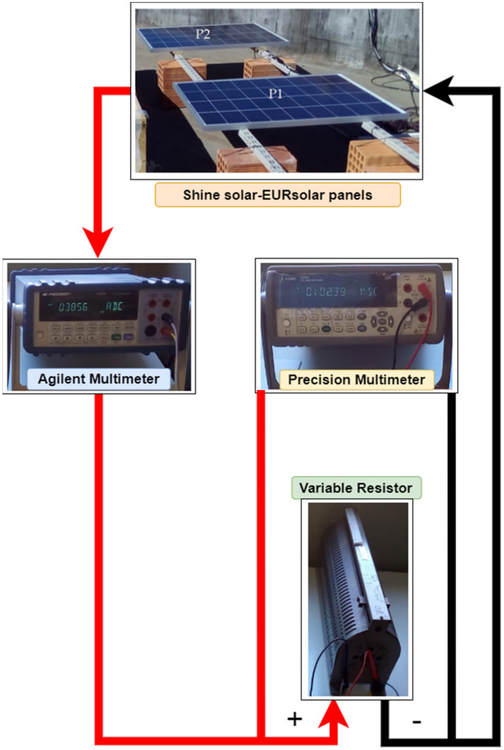
2.1. Instrumentation

Before starting the on-site measurements, the panels and the instruments were tested using artificial solar light, which has a maximum irradiance capacity of 1000 W/m² (see Section 3.1). On-site measurements were conducted during a period of 6 months. The instruments were set to measure at an interval of every one-minute.

Ambient parameters, e.g., wind velocity, temperature, atmospheric pressure, relative humidity, and precipitation were measured with the Vantage Pro weather station installed on the same roof as the test building near (approximately 2 m) the test apparatus. The solar insolation (total and diffused radiations) was measured using two separate pyranometers CMP11 (with sensitivity 8.45 μV/W/m²), and CM11 (with sensitivity 5.08 μV/W/m²) manufactured by KIPP & ZONEN company and are classified as “Secondary Standard” to comply with the requirements of ISO 9060 [30] ‘Solar energy’’.

The voltages of the PV panels P1 and P2 (The Shine Solar EURsolar −100 Wp with tolerance ±5) were measured and these data were further used to calculate the current and power produced, and therefore the generating efficiency. The voltages were measured, and the current was calculated based on the value of a fixed resistance i.e., 3.54 Ω (see the Section 2.4), used as load. To verify the panels performance and the influence of temperature on them, both panels were characterized, and I-V and P-V curves were obtained for different solar radiation ranges by using a variable resistance (see the Section 2.3).

An Agilent multi-meter and precision multi-meter (see Figure 3) have been used to measure current and voltage respectively while characterizing the PV panels. Both PV panels are equipped with thermocouples (Type -T) within the temperature range from −200 to 350 °C and sensitivity of about 43 μV/°C [31]. The temperature sensors underneath the panels were placed to measure respective working temperatures. The temperature sensors were completely sealed with cell synthetic rubbers and aluminum tape was put above the thermocouples to prevent outside heat and reflected radiation from affecting measurements.

The water surface temperatures were measured with the help of thermo-resistance temperature sensors (PT100 DIN-A manufactured by LSI S.p.a. with working temperature range of −50 to +600 °C), partially submerged by means of a specially made floating device (see Figure 2b).

All the measured data were collected continuously in two separate computers with the help of two data loggers, BABUC ABC and DEVIS PRO, placed inside the below laboratory.

2.2. Efficiency Evaluation

For the efficiency evaluation, the data collection and measurements were conducted in two phases: (1) In Phase I, the data were collected for both PV panels P1 and P2, with panel P1 placed inside the wooden basin without water; (2) in Phase II, the data were collected for both panels, but in this phase the wooden basin was filled with water and with panel P1 placed over the water surface.

The distance between the water surface level and the PV panel P1 was always maintained approximately to a distance of 7.5 cm, and panel P2 was mounted and placed outside the basin at ambient conditions.

2.3. Evaporation Estimation

For the evaporation estimation, the measurements were conducted in two phases separately with and without PV panel inside the wooden basin. To estimate the true daily evaporation rate, the experiments and measurements were conducted in summer months, considering the maximum evaporation generally occurs in these months.

To study the daily water evaporation measurement, a wooden basin of 2 × 2 m² was constructed and the PV panel P1 was placed inside the wooden basin and above water (as shown in Figure 1), covering approximately 17% of the basin’s total surface area. The water evaporation from this artificial water basin was monitored by measuring the level of water on a daily basis using a home-made measuring gauge, which follows the capillary method (as can be seen in the Figure 1b).

2.4. Efficiency Calculation and Choice of Load

The produced power and thereafter the efficiency of each PV panel at each instant (at a rate of per minute) were calculated, with respect to the measured voltage using Equation (1),

$$\mathsf{\eta }=\frac{\mathrm{P}}{({\mathrm{G}}_{\mathrm{Total}})\ast \left({\mathrm{A}}_{\mathrm{Panel}}\right)}$$

(1)

where η is the efficiency of each panel, P (W) is the produced power, G_Total (W/m²) the global irradiance, and A_Panel (m²) the net area of the PV panels. The choice of the loads was based on the theoretical capability to dissipate the maximum power produced by the panels, which can be calculated using Equation (2),

$${\mathrm{R}}_{\mathrm{MP}}=\frac{{\mathrm{V}}_{\mathrm{MP}}}{{\mathrm{I}}_{\mathrm{MP}}}$$

(2)

where R_MP (Ω) is the maximum resistance, V_MP (V) is the maximum voltage, and I_MP (A) is the maximum current.

The maximum rated power voltage and power current for the PV panels are 18.8 V and 5.3 A respectively, based on the data provided by the manufacturer.

Therefore, the calculated ideal resistances were used as load value equal to 3.54 Ω. The variable resistances have been used as loads for the PV panels.

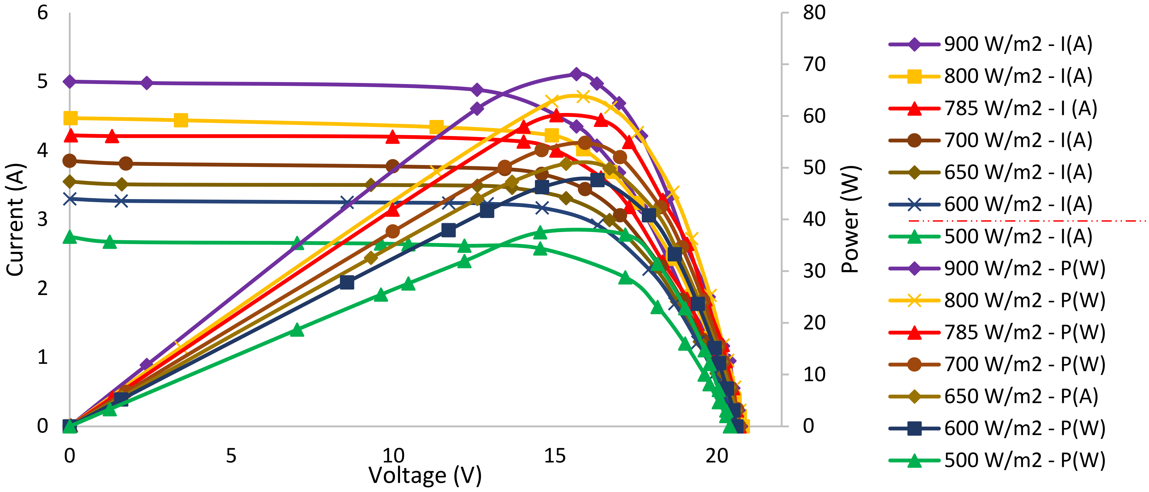
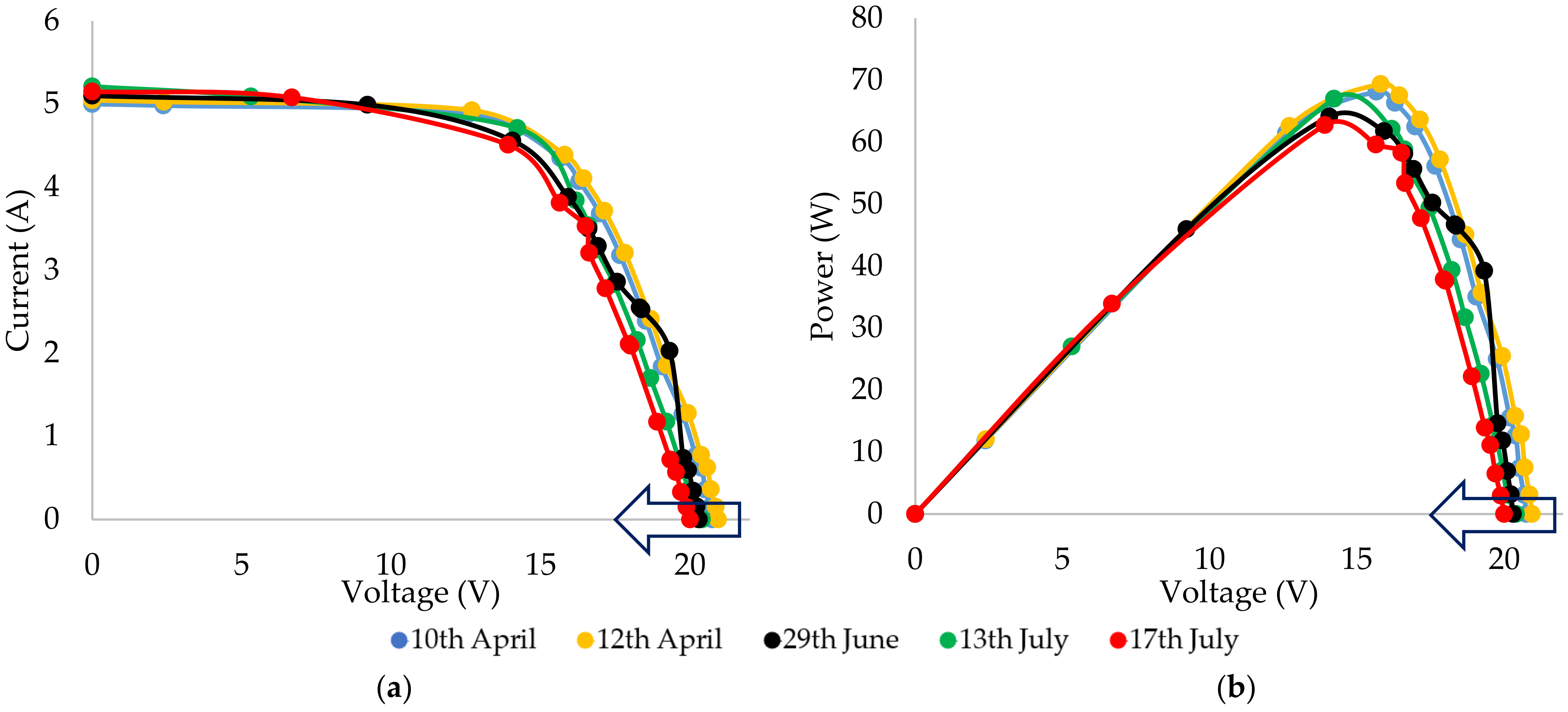
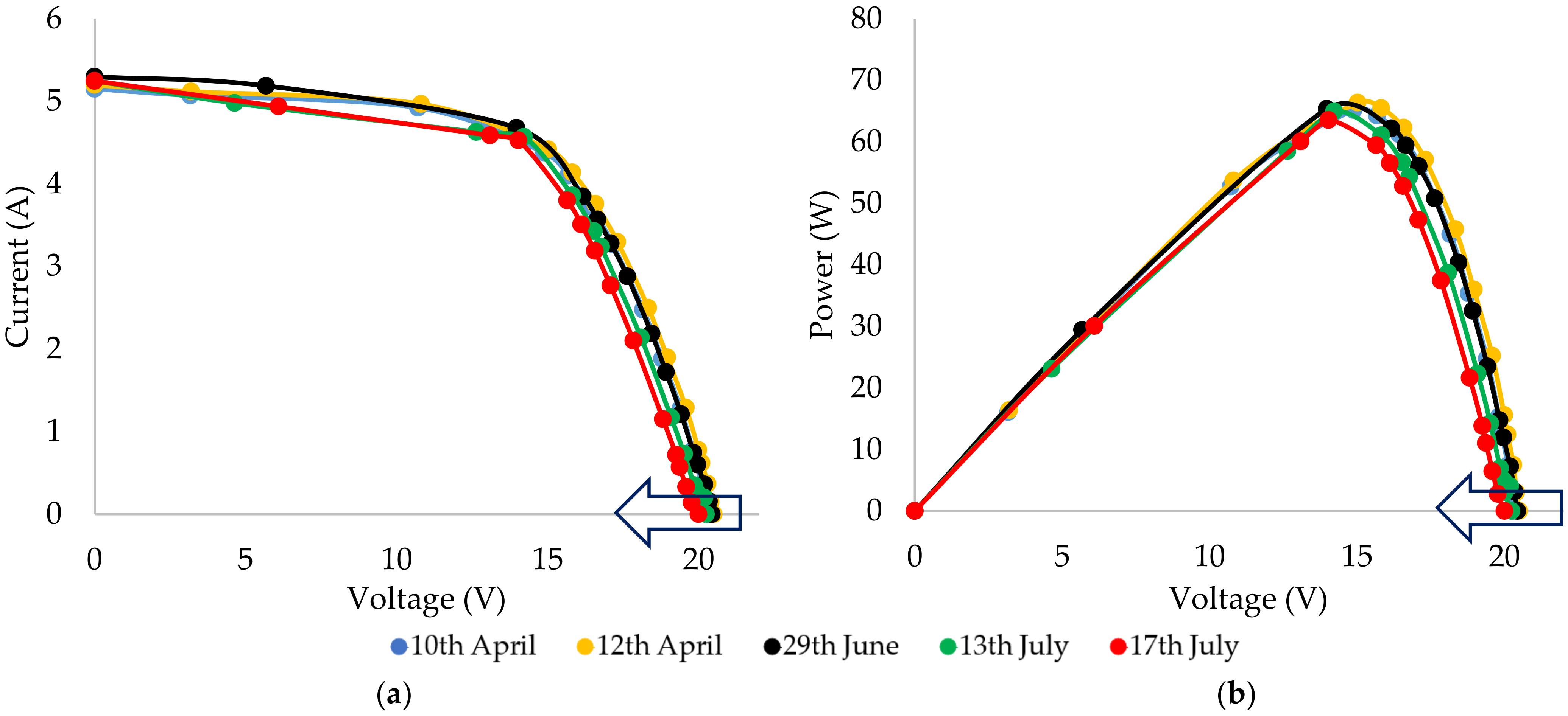
2.5. PV Panels Characteristic Curves

The PV panels characteristic curves (I-V and P-V) were plotted by measuring the voltages (V) and currents (A), with help of the Precision multi-meter and Agilent multi-meter (see Figure 3) respectively, by varying the resistance (Ω) of a variable resistor (see Figure 3).

Figure 4 demonstrates a typical trend of I-V and P-V curves of the panel P1 (100 Wp) at different solar irradiance from 500 to 900 W/m², for the measurements conducted on 10 April 2017 and the panel was placed in natural local ambient conditions with clear sky.

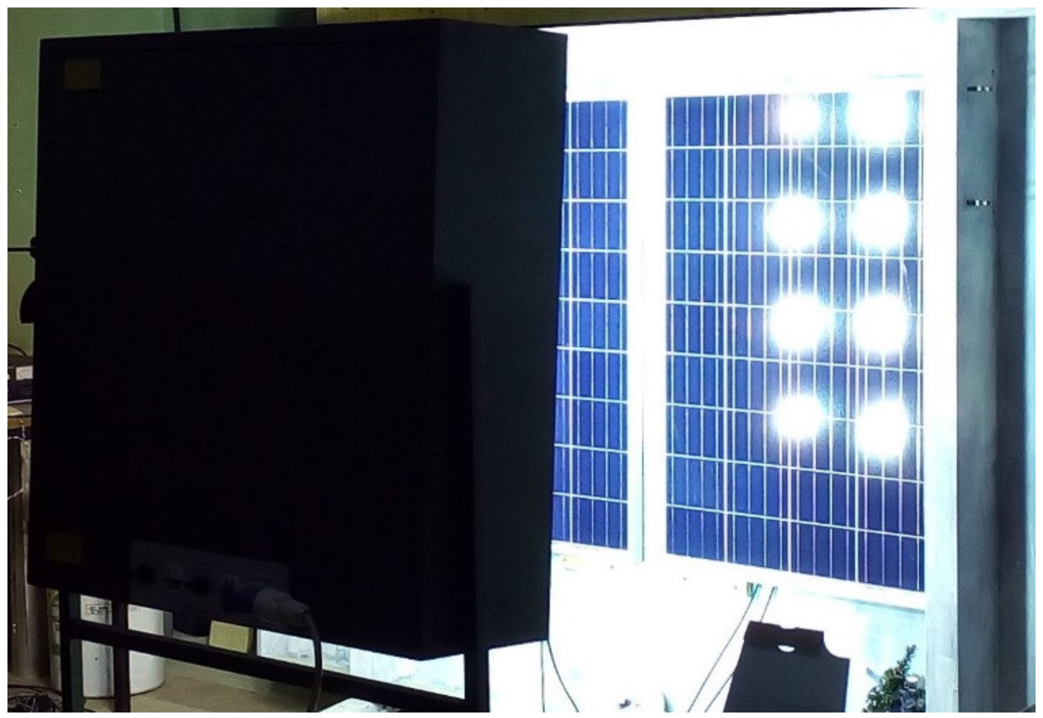
3. PV Panels—Performance Evaluation

At first, the PV panel performance was verified by using the solar simulator capable to perform long-term experiments under very stable conditions. It is composed of sixteen elliptical reflectors with Xenon short arc lamps (see Figure 5), altogether providing a power of 48 kW, replicating full spectrum sunlight with a flux density of 1000 W/m² and over 90% uniformity in the usable area.

The light source was placed one meter away from the targeted PV panel and single panel was tested individually, in the absence of diffused light or light source. In laboratory conditions, the measured open circuit voltage (Voc) of the panel (P1) was found to be 0.6% higher than that of panel (P2). Later, this difference has been used to adjust/eliminate the error from the measurements conducted in situ, natural ambient, and created conditions.

3.1. Under Normal Outdoor Conditions

Panel performance in situ with local ambient conditions and the effect of the temperature on the efficiency were analyzed. Panels were tested under same ambient condition (see Figure 6) and at identical reflection factors. For computing the characteristic curves, the measurements were carried out in April, June, and July, respectively, during the year 2017 (see

Table 1. Performance of the Panels at local ambient conditions @ 900 W/m².

	Ambient Conditions			Panels Temperature		Panels Performance
Tabulated Values Considered Here Are the Average of the Measured Data, Only in the Time Frame When the Available Global Irradiance Was 900 W/m2
				P1	P2	P1				P2
Test Date	Ta	RH	V	TP1	TP2	Measured Volt @ PMAX	Measured Current @ PMAX	PMAX	η	Measured Volt @ PMAX	Measured Current @ PMAX	PMAX	η
	°C	%	m/s	°C	°C	V	A	W		V	A	W
10 April	21.4	30	1.8	46.10	46.15	15.66	4.35	68.12	11.95%	14.88	4.38	65.19	11.57%
12 April	22.8	29	3.1	54.38	54.33	15.80	4.39	69.38	12.17%	15.02	4.42	66.39	11.65%
29 June	27.9	61	3.3	56.57	56.29	14.22	4.71	66.98	11.75%	13.97	4.68	65.38	11.47%
13 July	34.6	17	5.7	57.61	57.48	14.06	4.56	64.11	11.25%	14.22	4.57	64.99	11.40%
17 July	30.0	38	3.7	56.63	56.50	13.91	4.51	62.73	11.01%	14.03	4.53	63.56	11.15%

).

It is a well stablished fact that the PV panels do not use all the incident solar radiations to generate electrical energy. The photons with shorter wavelength contain higher energy and cannot free the electors to generate current. Therefore this un-usable energy gets dissipated as heat in the PV cell [32].

At high operating temperature, the PV panel’s efficiency decreases linearly so as the power output [33]. According to [34,35], the open circuit voltage also decreases with the increase in temperature and the same phenomenon was observed for the PV panels P1 and P2. In Figure 5, the IV and PV graphs of the PV panels were drawn with respect to the average solar irradiation of 900 W/m² and these trends are plotted from the zero voltage (at short circuit current Isc) to the open circuit voltage (Voc) by varying the load resistance, and each of these resistance points are represented on and along the trend lines in the graphs. The effect and the influence of the temperature on PV panels (P1 and P2) open circuit voltage is clearly noticeable in the I-V and P-V graphs (see Figure 7 and Figure 8). The trend curves and corresponding open circuit voltage shift towards lower voltages with an increase in ambient temperatures from about 20 °C in the month of April to approximately 30 °C measured in the month of July. Thereby, the maximum power of both panels was decreasing together with the calculated efficiency. For PV panel P1 and P2, the corresponding measured and calculated values for a particular solar irradiance (900 W/m²) and other local ambient conditions, are reported in Table 1.

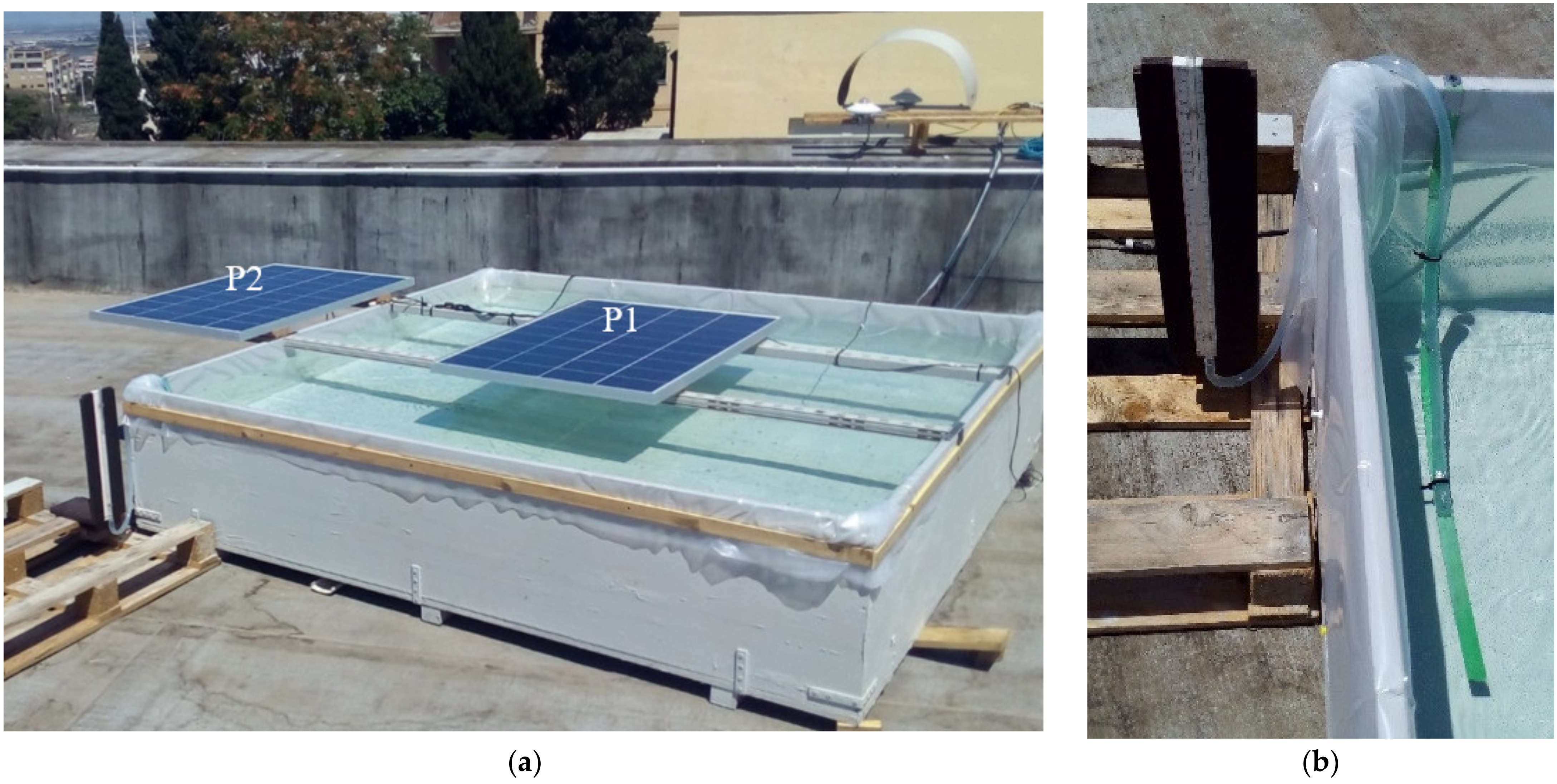
4. Situ Experimental Results, When P1 Placed on Water and P2 in Ambient Conditions

4.1. Temperature Reduction in the Panel (P1) Placed above the Water Surface

During phase I, the panel P1′s temperature always remained higher than that of panel P2, whereas just the opposite was observed during phase II.

During phase II, the temperature increment (from cooler to hotter months) of the panels found to be almost equal to the temperature different that was observed in phase I.

During phase II, the overall temperature drop of the panel P1 (with water underneath) occurred due to the water cooling process. Interestingly due to this passive water cooling, only the temperature of the panel P1 always remained lower than that of panel P2.

For each solar irradiation range, the temperature difference between panels P1 and P2 were calculated for both phase I and phase II. Based on the experimental observations and the above-mentioned considerations, the total reduction in temperature for panel P1 due to the convective cooling effect (passive water cooling) has been calculated and reported in

Table 2. P1’s Total temperature reduction (the panel under observation).

Global Radiation Ranges [W/m2]	Experiment—Phase I			Experiment—Phase II			The Total Reduction of Temp. [°C] for the Panel (P1)
	P1 Placed Inside the Wooden Basin WITHOUT Water	P2 Placed at Ambient Conditions		P1 Placed Inside the Wooden Basin WITH Water	P2 Placed at Ambient Conditions
	T P1 [°C]	T P2 [°C]	T P1 (pr.1) ↓	T P1 [°C]	T P2 [°C]	T P1 (pr.2) ↓	T P1 (Tot.temp) ↓
	When temp. of P1 > P2			When temp. of P1 < P2
	D	E	F = (D − E)	I	J	K = (I − J)	(−F) + (−K)
400 < G < 500	34.91	33.50	1.40	39.72	40.02	−0.31	−1.71
500 < G < 600	38.45	36.20	2.26	42.26	42.28	−0.02	−2.28
600 < G < 700	40.94	38.18	2.82	44.90	45.24	−0.34	−3.1
700 < G < 800	43.84	41.03	2.76	47.60	48.44	−0.84	−3.65
800 < G < 900	46.80	44.23	2.56	50.05	50.92	−0.87	−3.44
900 < G < 1000	48.99	47.07	1.93	52.21	53.10	−0.88	−2.81
1000 < G < 1100	45.87	44.40	1.47	49.96	50.71	−0.75	−2.22
1100 < G < 1200	45.78	44.23	1.55	52.64	54.02	−1.38	−2.93
Average	Reduction						−2.7

.

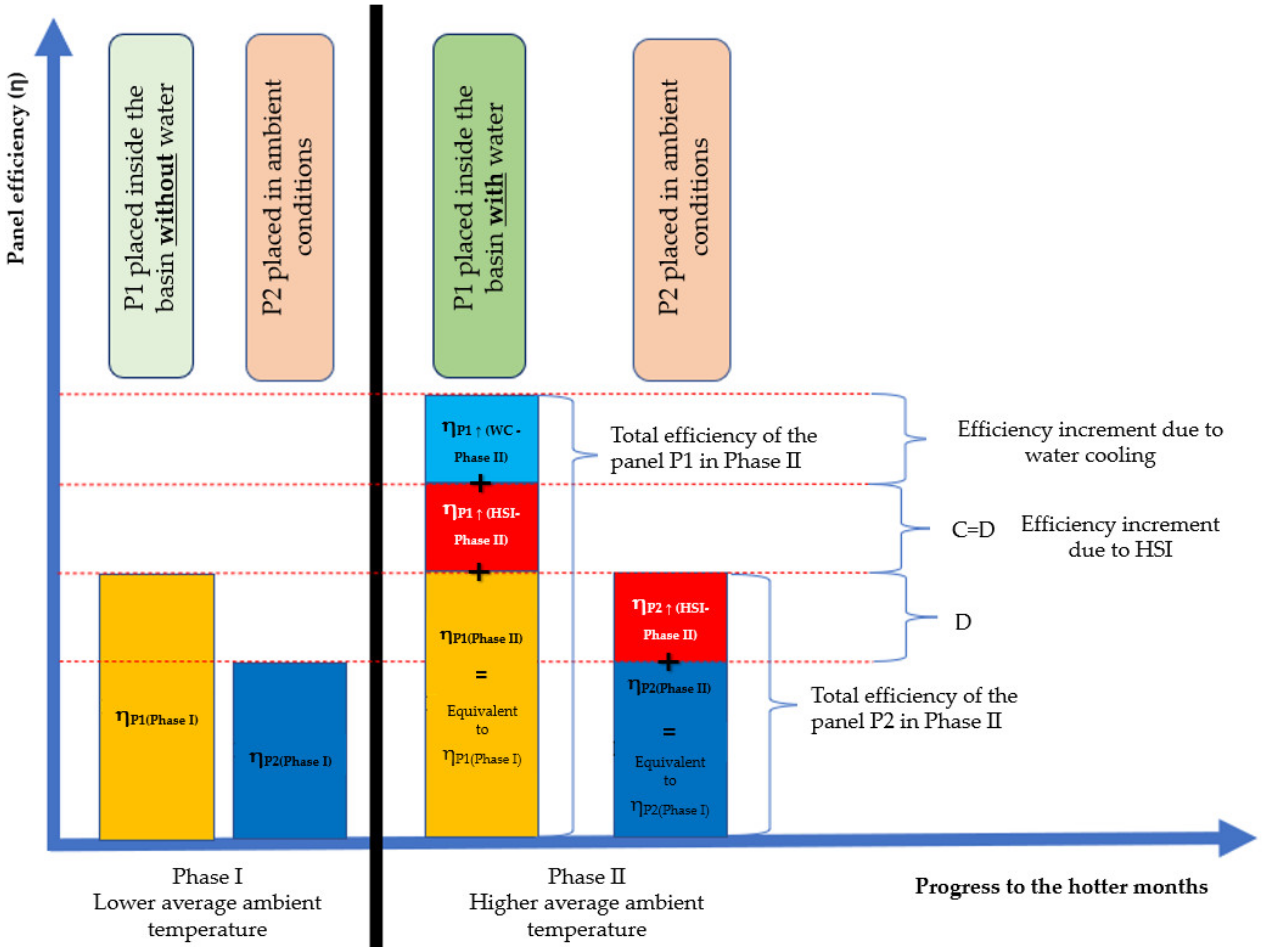
4.2. Efficiency Increment Calculation for P1 Panel

4.2.1. P1 and P2 Efficiencies during the Experiment Phase-I

In phase I, the panel P1 was placed horizontally inside the basin without any water, whereas the panel P2 was placed outside the basin with the same tilt angle, under normal ambient conditions. In this phase, the measured voltage data for both the panels were collected and these values were used to calculate the panels efficiencies. It is important to mention that the calculated efficiencies of the panels P1 and P2 were compared with each other at this stage only to demonstrate the similar behavior of the two panels as the solar radiation varies, with the same tilt angle but exposed to different reflecting surfaces (roof and basin). Thus, the efficiency of the panel P2 was used as a reference to evaluate the variation in efficiency due to the change in the local ambient conditions, especially due to the availability of higher solar irradiation (HSI) in the hotter months. In another way, it can be said that the change in the efficiency value of the panel P2 has been used to nullify the normal efficiency increment due to the HSI, from the total efficiency rise while calculating the real efficiency gain of P1 due to passive convective cooling. The calculated efficiencies during the experiment phase I of the panels P1 and P2 are designated as ${\mathsf{\eta }}_{\mathrm{P}1 \left(\mathrm{phase} \mathrm{I}\right)}$ and ${\mathsf{\eta }}_{\mathrm{P}2 \left(\mathrm{phase} \mathrm{I}\right)}$ in

Table 3. P1’s efficiency increment (the panel under observation).

	ηP1 [%] of the Panel under Observation (P1)			ηP2 [%] of the Panel under Observation (P2)
Global Radiation Ranges	Experiment—Phase-I Wooden Basin WITHOUT Water	Experiment—Phase-II Wooden Basin WITH Water	Efficiency Increment Due to Water Cooling Effect +Efficiency Increment Due to Change in the Ambient Conditions	Experiment—Phase-I Ambient Conditions	Experiment—Phase-II Ambient Conditions	Efficiency Increment Due to the Change in the Ambient Conditions	ηP1↑ TOTAL Increase in Efficiency [%]
	M	N	O = N − M	P	Q	R = Q − R	S = O − R
400 < G < 500	7.50%	9.70%	2.20%	6.70%	7.00%	0.30%	1.90%
500 < G < 600	8.70%	11.50%	2.80%	7.70%	8.40%	0.70%	2.10%
600 < G < 700	9.90%	13.30%	3.40%	8.90%	10.20%	1.30%	2.10%
700 < G < 800	10.70%	14.20%	3.50%	10.10%	11.60%	1.50%	2.00%
800 < G < 900	11.30%	14.20%	2.90%	10.90%	11.90%	1.00%	1.90%
900 < G < 1000	11.50%	13.60%	2.10%	11.00%	11.50%	0.50%	1.60%
1000 < G < 1100	11.20%	13.20%	2.00%	10.60%	11.30%	0.70%	1.30%
1100 < G < 1200	10.50%	12.30%	1.80%	9.90%	10.60%	0.70%	1.10%
Avg.	10.16%	12.75%	2.59%	9.48%	10.31%	0.84%	1.75%

.

4.2.2. P1 and P2 Efficiencies during the Experiment Phase-II

During the phase II experiment-period, the water height below panel P1 was constantly monitored and maintained apparently at a fixed level by adding the equivalent amount of water evaporated on a daily basis. The distance between the water surface and the panel P1 was kept approximately at 7.5 cm. Meanwhile, panel P2 was kept in the same place and position as in phase I.

The simplified form of the efficiencies of the panel P1 and P2, during the phase II could expressed as ${\mathsf{\eta }}_{\mathrm{P}1 \left(\mathrm{phase} \mathrm{II}\right)}$ and ${\mathsf{\eta }}_{\mathrm{P}2 \left(\mathrm{phase} \mathrm{II}\right)}$ (see Equations(3) and (4)), and represented as R and Q respectively in the Table 3.

As is evident in Table 3, during phase II, the efficiency increment of panel P1 was higher than that of panel P2. Moreover, the efficiencies of the panels P1 and P2 observed during the experiment phase II was found always to be higher than that of phase I.

Based on the above-mentioned observations, the efficiencies of the panels P1 and P2 during phase II could be equated as follows. At first, the efficiency increment of P1 and P2 during phase II can be assumed to be equal to the sum of the efficiency obtained during phase I and the efficiency increment due to external effects (like higher HSI and water cooling etc.)

While plotting the graph (Figure 9), the measured voltage and current values obtained within the global radiation range from 400 < G < 500 W/m² to 1100 < G < 1200 W/m² were considered.

Now, the efficiencies attended by both panels during phase II could be written as,

$${\mathsf{\eta }}_{\mathrm{P}1 \left(\mathrm{phase} \mathrm{II}\right)}={\mathsf{\eta }}_{\mathrm{P}1 \left(\mathrm{phase} \mathrm{I}\right)}+{\mathsf{\eta }}_{\mathrm{P}1\uparrow \left(\mathrm{phase} \mathrm{II}\right)}$$

(3)

$${\mathsf{\eta }}_{\mathrm{P}2 \left(\mathrm{phase} \mathrm{II}\right)}={\mathsf{\eta }}_{\mathrm{P}2 \left(\mathrm{phase} \mathrm{I}\right)}+{\mathsf{\eta }}_{\mathrm{P}2\uparrow \left(\mathrm{phase} \mathrm{II}\right)}$$

(4)

where ${\mathsf{\eta }}_{\mathrm{P}1\uparrow \left(\mathrm{phase} \mathrm{II}\right)}$ and ${\mathsf{\eta }}_{\mathrm{P}2\uparrow \left(\mathrm{phase} \mathrm{II}\right)}$ represent the efficiency increment of panel P1 and P2, respectively, due to the higher solar irradiation and water cooling for panel P1 and only to higher solar irradiation for panel P2.

From Equation (4), the total efficiency increment ${\mathsf{\eta }}_{\mathrm{P}1\uparrow \left(\mathrm{phase} \mathrm{II}\right)}$ of the panel P1, from phase I to phase II can be written as,

$${\mathsf{\eta }}_{\mathrm{P}1\uparrow \left(\mathrm{phase} \mathrm{II}\right)}=\left[{\mathsf{\eta }}_{\mathrm{P}1 \left(\mathrm{phase} \mathrm{II}\right)}-{\mathsf{\eta }}_{\mathrm{P}1 \left(\mathrm{phase} \mathrm{I}\right)}\right]$$

(5)

In another way, assuming a reasonable linear combination of effects, the same efficiency increment of the panels P1, during the experiment phase II can be expressed as,

$${\mathsf{\eta }}_{\mathrm{P}1 \uparrow \left(\mathrm{phase} \mathrm{II}\right)}={\mathsf{\eta }}_{\mathrm{P}1 \uparrow \left(\mathrm{HSI}\right)}+{\mathsf{\eta }}_{\mathrm{P}1 \uparrow \left(\mathrm{WC}\right)}$$

(6)

where,

${\mathsf{\eta }}_{\mathrm{P}1 \uparrow \left(\mathrm{HSI}\right)}$ is the efficiency increment due to availability of HSI during successive summer and longer months, and other respective ambient conditions.

${\mathsf{\eta }}_{\mathrm{P}1 \uparrow \left(\mathrm{WC}\right)}$ is the efficiency gain due to passive water cooling (WC).

Similarly, the total efficiency increment ${\mathsf{\eta }}_{\mathrm{P}2 \uparrow \left(\mathrm{phase} \mathrm{II}\right)}$ of the panel P2 from phase I to phase II should be equal to (using the Equation (4)),

$${\mathsf{\eta }}_{\mathrm{P}2 \uparrow \left(\mathrm{phase} \mathrm{II}\right)}=\left[{\mathsf{\eta }}_{\mathrm{P}2 \left(\mathrm{phase} \mathrm{II}\right)}-{\mathsf{\eta }}_{\mathrm{P}2 \left(\mathrm{phase} \mathrm{I}\right)}\right]={\mathsf{\eta }}_{\mathrm{P}2 \uparrow \left(\mathrm{HSI}\right)}$$

(7)

In Equation (7), ${\mathsf{\eta }}_{\mathrm{P}2 \uparrow \left(\mathrm{WC}\right)}$ = 0, as panel P2 was placed in ambient condition and away from the influence of the water.

${\mathsf{\eta }}_{\mathrm{P}1 \uparrow \left(\mathrm{HSI}\right)}$ is the efficiency increment due to the availability of HSI during successive summer and longer months, and other respective ambient conditions.

As mentioned previously, panel P2 was used as reference with the objective to have only the efficiency amount that is influenced due to the local ambient conditions. Finally, the similar behavior of the two panels when the solar radiation varies (see Section 4.2.1), allows to obtain,

$${\mathsf{\eta }}_{\mathrm{P}1 \uparrow \left(\mathrm{HSI}\right)}={\mathsf{\eta }}_{\mathrm{P}2 \uparrow \left(\mathrm{HSI}\right)}$$

(8)

4.2.3. Total Efficiency Increment Due to Water Cooling of P1

The total efficiency increment due to passive water cooling ${\mathsf{\eta }}_{\mathrm{P}1\uparrow \left(\mathrm{WC}\right)}$ taking into account Equation (5), can be written as,

$${\mathsf{\eta }}_{\mathrm{P}1\uparrow \left(\mathrm{WC}\right)}={\mathsf{\eta }}_{\mathrm{P}1 \uparrow \left(\mathrm{phase} \mathrm{II}\right)}-{\mathsf{\eta }}_{\mathrm{P}1 \uparrow \left(\mathrm{HSI}\right)}$$

(9)

which, combining with Equations (7), (8) and (10), one obtains,

$${\mathsf{\eta }}_{\mathrm{P}1 \uparrow \left(\mathrm{Total} \mathrm{WC}\right)}=\left[{\mathsf{\eta }}_{\mathrm{P}1 \left(\mathrm{phase} \mathrm{II}\right)}-{\mathsf{\eta }}_{\mathrm{P}1 \left(\mathrm{phase} \mathrm{I}\right)}\right]-\left[{\mathsf{\eta }}_{\mathrm{P}2 \left(\mathrm{phase} \mathrm{II}\right)}-{\mathsf{\eta }}_{\mathrm{P}2 \left(\mathrm{phase} \mathrm{I}\right)}\right]$$

(10)

5. Evaporation Reduction Estimation

Water evaporation from the basin was measured and thereafter calculated by using the water budget method, when all components of the water budget except evaporation are either measured or estimated over a time-period (t) [36].

$$E_o=Q_i+P-Q_o- \Delta S$$

(11)

where,

E_o (m³/t) is the evaporation from the wooden basin under observation.

P (m³/t) is the precipitation on the basin, null during the experimental period.

Q_i and Q_o (m³/t) are the water in and out flows respectively, according to the water balance method.

The experimental structure under observation was placed above a rooftop, isolated, and insulated. Thus, there was no in or out flow of water and all the values respective to Q_i and Q_o can be neglected. We used Q_INPUT as the initial volume of water inside the basin. ΔS (m³/t) is the change in the storage and was measured regularly.

After all the above considerations, Equation (11) was modified to have the new water balance formula, shown as below:

$$E_o=Q_{INPUT}-(h_x\ast A_{SB})$$

(12)

where h_x (m) is the average level of water inside the basin. The h_x inside the wooden basin was determined through eight measurements at different points inside the same basin. A_SB (m²) represents the water surface area inside the basin.

The water inside the artificial wooden basin was poured manually and the initial water volume inside the basin can be written as, $Q_{INPUT}=Q_{INITIAL}=(h_{INITIAL}\ast A_{SB})$ and initial water level is given as $h_x=h_{INITIAL}$.

Water evaporation rate was measured on a daily basis by using our own home-made evaporation meter (see Figure 1b), which was constructed following the communicating vessels principle. The water evaporation was calculated based on the difference measured between the basin with and without the panel P1.

6. Results and Discussion

Three different but correlating effects have been observed during this study: (i) the temperature reduction of the panel P1 inside the basin, when water was present underneath the panel (for details, see Section 4.1), (ii) increment in the panel P1’s overall generating efficiency (for details, see Section 4.2), and (iii) reduction in water evaporation due to the presence of panel P1 inside the wooden basin (for details, see Section 5).

6.1. Temperature Effect

The heating-up of the solar panel was also responsible for the heating of the surrounding air, whereas the hot air underneath the panel remained blocked due the metal structural frame of the panel and was thus unable to rise-up [32] or circulate. This phenomenon is responsible in rising the temperature of the panel.

During the temperature analysis of PV panels in the experimental phase I, it was observed that the panel P1 inside the wooden basin without water always maintained a higher value of temperature than that of panel P2, with the difference ranging from 1.40 to 2.82 °C, and the highest value was measured in 700–800 W/m² range (see Table 2). The higher value of temperatures of the panel P1 could be associated to the lack of free air flow underneath the panel, and due to it being placed in an enclosed environment inside the wooden basin. In contrast, panel P2 was placed at normal ambient conditions, thus enjoying a continuous flow of fresh air from the surroundings which might have helped it to keep its temperature lower than that of panel P1.

The experimental phase II was performed during the summer period, and due to the availability of HSI and corresponding rising ambient temperature, we noted the measured temperatures of both panels to be higher than that of measurements conducted during phase I (see Figure 7 and Table 2), specifically when compared with their own measured values. Notably, during this phase, when the panel P1 was placed inside the water-filled wooden basin and the panel P1′s temperature always remained lower (in the range of 0.02–1.38 °C) than that of P2, the exact opposite to that which was noticed during phase I occurred (see Table 2).

As highlighted in [19,37], due to the phenomenon of the water-cooling effect, the ambient temperature above the water surface would be lower than the temperature on land. So, as panel P1 was placed above water, the hot air-temperature under the panel and cooler ambient-temperature above water would have created the air circulation underneath the panel and therefore, it leads to a natural air-convection underneath the panel P1. This phenomenon predominantly accounts for the passive cooling of the panel P1 and temperature reduction, and it certainly must have had an influence in lowering the panel P1’s temperature (see Figure 10, Table 2). The maximum reduction of 3.7 °C in panel P1’s temperature was noticed in the range of 700–800 W/m², whereas an average reduction of 2.3 °C was achieved for the same panel due to water cooling.

6.2. Efficiency Increment

During the consecutive experiment phases, it was observed that the efficiency of both the panels increased continuously and simultaneously. One of the experimental objectives was to increase the overall electricity production and improve the generating efficiency of the PV panel (i.e., of P1), through convective natural cooling, specifically by raising it over water.

PV panel P2 was used as a reference panel and it was kept in a fixed position, away from the influence of water, throughout the project period.

The panel P2’s efficiency increment from phase I to phase II was only influenced by the change in the ambient conditions like colder months (phase I’s average efficiency of 9.48%) to hotter months with HSI (phase I’s average efficiency of 10.31%). Therefore, on average, the total efficiency improvement observed only due to the natural phenomenon was 0.75%.

On the other hand, panel P1’s efficiency increment was due to the water cooling effect as well as the change in the ambient conditions (similar as of P2), and an efficiency increment from phase I (12.16%) to phase II (12.75%) was found (see Table 3). When calculating the efficiency increment of panel P1 only due to the water cooling effect, this improvement was found to be 1.75% (absolute), with a maximum increment of 2.10% observed in the radiation ranges of 600–700 W/m² and 700–800 W/m².

The efficiency improvement of the panel P1 expressed in relative terms was found to be equal to 17.22% on an average (i.e., from 10.16% to 11.91% = 12.75–0.84%), and this improvement was due to passive water cooling. Figure 11 demonstrates the efficiency increment in correspondence of each solar radiation category, for the cases when panel P1 was put inside the wooden basin without water (in the phase I) and then filled with water (in the phase II).

6.3. Water Evaporation Reduction

Based on the daily measurements of the water evaporation from the basin with and without panel P1, the evaporation rate was calculated by using the water balance method. It was found that only by covering approximately 17% of the total water surface area (see Figure 3), approximately 30% of water evaporation from the basin could be reduced.

6.4. Efficiency and Evaporation-Integrated Approach

The experiment has demonstrated that this integrated approach helps to improve the panel’s (P1) efficiency by almost 1.75% (absolute), i.e., around 17% (relative), through passive water cooling. Therefore, reducing the panel (P1) temperature by about 2.7 °C (avg.) also helps to keep the valuable water in the basin by minimizing the water loss through evaporation.

7. Conclusions

This paper analyses the dual positive effects of raising PV panels above water, specifically to improve the panel’s generating efficiency induced by passive cooling from water underneath the PV panel and the reduction in water evaporation achieved by creating an artificial shadow of the same panel above the water. By studying the two effects simultaneously, our research effort is unique and novel, as previously published works have either investigated PV panel efficiency increment achieved through active or passive cooling or have examined the data related to water evaporation. Therefore, no experimental data are available highlighting these two aspects together. The present work demonstrates that passive underneath water cooling of the panel reduces the panel’s operating temperature by approximately 2.7 °C (on average), and with a maximum of 3.7 °C for 700 < G < 800 W/m² range. The water-cooling process facilitated improving the panel’s efficiency by 1.75% (absolute), i.e., around 17.22% (relative), and the shadowing effect reduced the water evaporated from the basin by 30%.

In conclusion, the information gathered in this study could encourage developers and nations to install PV system(s) on water (i.e., water bodies) as it is an ingenious system. With proper design, it could be possible to increase the total energy production while at the same time reducing water evaporation and therefore also reducing the land stress.

Even though the outcome of this experiment conducted in a 3–4-month period provides encouraging results, large-scale experiments need to be undertaken for an arc of at least a year (considering all seasons) to better estimate the performance of the PV panel and its influence on the marine eco-system.

References

1. Krumdieck, S. Transition Engineering- Building a Sustainable Future; CRC Press: Boca Raton, FL, USA, 19 September 2019. [Google Scholar] [CrossRef]
2. Razak, A.; Irwan, Y.M.; Leow, W.Z.; Irwanto, M.; Safwati, I.; Zhafarina, M. Investigation of the effect temperature on photovoltaic (PV) panel output performance. Int. J. Adv. Sci. Eng. Inf. Technol. 2016, 6, 682–688. [Google Scholar] [CrossRef]
3. Arpino, F.; Cortellessa, G.; Frattolillo, A. Experimental and numerical assessment of photovoltaic collectors performance dependence on frame size and installation technique. Sol. Energy 2015, 118, 7–19. [Google Scholar] [CrossRef]
4. Dubey, S.; Sarvaiya, J.N.; Seshadri, B. Temperature dependent photovoltaic (PV) efficiency and its effect on PV production in the world—A review. Energy Procedia 2013, 33, 311–321. [Google Scholar] [CrossRef] [Green Version]
5. Grubišić-Čabo, F.; Nižetić, S.; Giuseppe Marco, T. Photovoltaic panels: A review of the cooling techniques. Trans. FAMENA 2016, 40, 63–74. [Google Scholar]
6. Bijjargi, Y.S.; Kale, S.S.; Shaikh, K.A. Cooling techniques for photovoltaic module for improving its conversion efficiency: A review. Int. J. Mech. Eng. Technol. (IJMET) 2016, 7, 22–38. [Google Scholar]
7. Mazón-Hernández, R.; García-Cascales, J.R.; Vera-García, F.; Káiser, A.S.; Zamora, B. Improving the electrical parameters of a photovoltaic panel by means of an induced or forced air stream. Int. J. Photoenergy 2013, 2013, 830968. [Google Scholar] [CrossRef]
8. Gang, P.; Huide, F.; Huijuan, Z.; Jie, J. Performance study and parametric analysis of a novel heat pipe PV/T system. Energy 2012, 37, 384–395. [Google Scholar] [CrossRef]
9. Maiti, S.; Banerjee, S.; Vyas, K.; Patel, P.; Ghosh, P.K. Self regulation of photovoltaic module temperature in V-trough using a metal–wax composite phase change matrix. Sol. Energy 2011, 85, 1805–1816. [Google Scholar] [CrossRef]
10. Arcuri, N.; Reda, F.; De Simone, M. Energy and thermo-fluid-dynamics evaluations of photovoltaic panels cooled by water and air. Sol. Energy 2014, 105, 147–156. [Google Scholar] [CrossRef]
11. Ueda, Y.; Sakurai, T.; Tatebe, S.; Itoh, A.; Kurokawa, K. Performance analysis of PV systems on the water. In Proceedings of the 23rd European Photovoltaic Solar Energy Conference, Valencia, Spain, 1 September 2008; pp. 2670–2673. [Google Scholar]
12. Dorobanţu, L.; Popescu, M.O. Increasing the efficiency of photovoltaic panels through cooling water film. UPB Sci. Bull. Ser. C 2013, 75, 223–232. [Google Scholar]
13. Hachicha, A.A.; Ghenai, C.; Hamid, A.K. Enhancing the performance of a photovoltaic module using different cooling methods. World Acad. Sci. Eng. Technol. Int. J. Environ. Chem. Ecol. Geol. Geophys. Eng. 2015, 9, 1106–1109. [Google Scholar]
14. Rosa-Clot, M.; Tina, G.M. Submerged and Floating Photovoltaic Systems: Modelling, Design and Case Studies; Academic Press: Cambridge, MA, USA, 2017; ISBN 9780128123232, Paperback ISBN 9780128121498. [Google Scholar]
15. Abdulgafar, S.A.; Omar, O.S.; Yousif, K.M. Improving the efficiency of polycrystalline solar panel via water immersion method. Int. J. Innov. Res. Sci. Eng. Technol. 2014, 3, 96–101. [Google Scholar]
16. Trapani, K. Flexible Floating Thin Film Photovoltaic (PV) Array Concept for Marine and Lacustrine Environments. Ph.D. Thesis, Laurentian University of Sudbury, Sudbury, ON, Canada, 2014. [Google Scholar]
17. Redón-Santafé, M.; Ferrer-Gisbert, P.S.; Sánchez-Romero, F.J.; Torregrosa Soler, J.B.; Gozalvez, F.; Javier, J.; Ferrer Gisbert, C.M. Implementation of a photovoltaic floating cover for irrigation reservoirs. J. Clean. Prod. 2014, 66, 568–570. [Google Scholar] [CrossRef] [Green Version]
18. Sahu, A.; Yadav, N.; Sudhakar, K. Floating photovoltaic power plant: A review. Renew. Sustain. Energy Rev. 2016, 66, 815–824. [Google Scholar] [CrossRef]
19. Liu, L.; Wang, Q.; Lin, H.; Li, H.; Sun, Q. Power generation efficiency and prospects of floating photovoltaic systems. Energy Procedia 2017, 105, 1136–1142. [Google Scholar] [CrossRef]
20. Choi, Y.K. A study on power generation analysis of floating PV system considering environmental impact. Int. J. Softw. Eng. Its Appl. 2014, 8, 75–84. [Google Scholar] [CrossRef]
21. Floating Photovoltaic. Available online: http://www.nrg-energia.it/fotovoltaico-galleggiante.html (accessed on 7 December 2021).
22. Thi, N.D. The Evolution of Floating Solar Photovoltaics; Research Gate: Berlin, Germany, 16 July 2017. [Google Scholar]
23. Rosa-Clot, M.; Tina, G.M.; Nizetic, S. Floating photovoltaic plants and wastewater basins: An Australian project. Energy Procedia 2017, 134, 664–674. [Google Scholar] [CrossRef]
24. Sukhatme, S.P. Meeting India’s future needs of electricity through renewable energy sources. Curr. Sci. 2011, 101, 624–630. [Google Scholar]
25. Piano, S.L.; Mayumi, K. Toward an integrated assessment of the performance of photovoltaic power stations for electricity generation. Appl. Energy 2017, 186, 167–174. [Google Scholar] [CrossRef] [Green Version]
26. Martín-Chivelet, N. Photovoltaic potential and land-use estimation methodology. Energy 2016, 94, 233–242. [Google Scholar] [CrossRef]
27. Vörösmarty, C.J.; Green, P.; Salisbury, J.; Lammers, R.B. Global water resources: Vulnerability from climate change and population growth. Science 2000, 289, 284–288. [Google Scholar] [CrossRef] [PubMed] [Green Version]
28. Mekonnen, M.M.; Hoekstra, A.Y. Four billion people facing severe water scarcity. Sci. Adv. 2016, 12, e1500323. [Google Scholar] [CrossRef] [PubMed] [Green Version]
29. Taboada, M.E.; Cáceres, L.; Graber, T.A.; Galleguillos, H.R.; Cabeza, L.F.; Rojas, R. Solar water heating system and photovoltaic floating cover to reduce evaporation: Experimental results and modeling. Renew. Energy 2017, 105, 601–615. [Google Scholar] [CrossRef] [Green Version]
30. ISO-9060. Solar Energy—Specification and Classification of Instruments for Measuring Hemispherical Solar and Direct Solar Radiation; International Organization for Standardization: Geneva, Switzerland, 2018. [Google Scholar]
31. Pandya, R. To Study and Used of Thermocouple for Temperature Measurement in Experiment Work. Vol-1 Issue-4 2015. JARIIE-ISSN(O)-2395-4396. Available online: http://ijariie.com/AdminUploadPdf/TO_STUDY_AND_USED_OF_THERMOCOUPLE_FOR_TEMPERATURE_MEASURMENT_IN_EXPERIMENT_WORK_ijariie1293_volume_1_14_page_181_190.pdf (accessed on 7 December 2021).
32. Abdelhady, S.; Abd-Elhady, M.S.; Fouad, M.M. An understanding of the operation of silicon photovoltaic panels. Energy Procedia 2017, 113, 466–475. [Google Scholar] [CrossRef]
33. Tobnaghi, D.M.; Madatov, R.; Naderi, D. The effect of temperature on electrical parameters of solar cells. Int. J. Adv. Res. Electr. Electron. Instrum. Eng. 2013, 2, 6404–6407. [Google Scholar]
34. Abd-Elhady, M.S.; Serag, Z.; Kandil, H.A. An innovative solution to the overheating problem of PV panels. Energy Convers. Manag. 2018, 157, 452–459. [Google Scholar] [CrossRef]
35. Nelson, J. The Physics of Solar Cells; Imperial College Press: London, UK, 2003; ISBN 978-1-86094-340-9. [Google Scholar]
36. Brooks, K.N.; Ffolliott, P.F.; Magner, J.A. Hydrology and the Management of Watersheds; John Wiley & Sons: Hoboken, NJ, USA, October 2012. [Google Scholar] [CrossRef]
37. Wang, H.; Fu, B. The temperature effect of water body. Meteorol. Sci. 1991, 11, 233–243. [Google Scholar]
Figure 1. (a) PV Panel P1 placed above water surface, whereas the Panel P2 placed at ambient condition; (b) Water evaporation measuring system.
Energies 14 08336 g001
Figure 2. Measurement variables and instruments for experimental set-up. (a) pyranometer for global and diffuse radiation; (b) RTD for water temperature and (c) Thermocouple to measure the panel temperature.
Energies 14 08336 g002
Figure 3. PV panels characterization scheme.
Energies 14 08336 g003
Figure 4. PV panel P1’s characteristics curves (I-V and P-V).3. PV panels characterization at laboratory and ambient conditions.
Energies 14 08336 g004
Figure 5. Panels tested with solar simulator at laboratory condition.
Energies 14 08336 g005
Figure 6. Panels placed under identical condition.
Energies 14 08336 g006
Figure 7. I-V and P-V curves for PV panel P1. (a) Temperature effect on PV panel P1 and the I-V curves behavior at 900 W/m2 with different ambient temperatures, (b) Temperature effect on P1and the P-V curves behavior at 900 W/m2 with different ambient temperatures (see Table 1).
Energies 14 08336 g007
Figure 8. I-V and P-V curves for PV panel P2. (a) Temperature effect on P2 and the IV curves behavior at 900 W/m2 with different ambient temperatures, (b) Temperature effect on P2 and the PV curves behavior at 900 W/m2 with different ambient temperatures (see the Table 1).
Energies 14 08336 g008
Figure 9. Panels efficiency increment scheme, in phase II- two phenomenon have affected the efficiency increment (1) availability of higher solar insolation (increment observed in both panels) and (2) due to water cooling effect (only observed in the case of P1 placed above water).
Energies 14 08336 g009
Figure 10. Temperature reduction due to water cooling- temperature variation of the panels.
Energies 14 08336 g010
Figure 11. The efficiency increment of the PV panel P1.
Energies 14 08336 g011