Article

Rotating Instabilities in a Low-Speed Single Compressor Rotor Row with Varying Blade Tip Clearance

1
Chair of Turbomachinery and Flight Propulsion, Technische Universität Dresden, 01062 Dresden, Germany
2
School of Power and Energy, Northwestern Polytechnical University, Xi’an 710129, China
*
Author to whom correspondence should be addressed.
Energies 2021, 14(24), 8369; https://doi.org/10.3390/en14248369
Submission received: 18 November 2021 / Revised: 6 December 2021 / Accepted: 9 December 2021 / Published: 12 December 2021

Abstract

:
When a compressor is throttled to the near stall point, rotating instability (RI) is often observed as significant increases of amplitude within a narrow frequency band which can be regarded as a pre-stall disturbance. In the current study, a single compressor rotor row with varying blade tip clearance (1.3%, 2.6% and 4.3% chord length) was numerically simulated using the zonal large eddy simulation model. The mesh with six blade passages was selected to capture the proper dynamic feature after being validated in comparison to the measured data, and the dynamic mode decomposition (DMD) approach was applied to the numerical temporal snapshots. In the experimental results, RIs are detected in the configurations with middle and large tip gaps (2.6% and 4.3% chord length), and the corresponding characterized frequencies are about 1/2 and 1/3 of the blade passing frequency, respectively. Simulations provide remarkable performance in capturing the measured flow features, and the DMD modes corresponding to the featured RI frequencies are successfully extracted and then visualized. The analysis of DMD results indicates that RI is essentially a presentation of the pressure wave propagating over the blade tip region. The tip leakage vortex stretches to the front part of the adjacent blade and consequently triggers the flow perturbations (waves). The wave influences the pressure distribution, which, in turn, determines the tip leakage flow and finally forms a loop.

1. Introduction

Rotating instability (RI) is one of the typical dynamic properties in compressors. This phenomenon is observed near the stability limit of the compressor and can be regarded as a pre-stall disturbance [1]. In the frequency spectra processed from casing wall pressure, RIs are found as significant increases of amplitude within a narrow frequency band below the blade passing frequency (BPF). The circumferential mode order of RI varies from 1/3 to 2 times the rotor blade number, and the rotating velocity of RI is from 25% to 90% of the rotor velocity [2].
RI has been detected in a variety of turbomachines. Early in the 1980s, Mathioudakis and Breugelmans [3] noticed the existence of the RI disturbance in a low-speed axial compressor. Later on, Liu et al. [4] performed measurements on a low-speed axial fan and found a narrow-band tip clearance noise component below BPF when the tip clearance was larger than or equal to 0.27% of the impeller diameter. They also concluded that the mode orders of the disturbance and rotating stall are not harmonically related. Based on the same test rig, Kameier and Neise [5] discovered that the pressure level increases within narrow frequency bands in a region below BPF when the tip clearance is enlarged, and RI only occurs if a reversed flow condition exists in the tip gap. Based on the Dresden Low Speed Research Compressor (LSRC), Mailach et al. [2,6] carried out experiments on a 4-stage axial compressor with varying blade tip clearance only for the third rotor row and a linear cascade using the same rotor blades, respectively. The RIs were found in those configurations with relatively large tip clearance. Rolfes et al. [7] observed RI in a single stage build of the Dresden LSRC when the rotor tip clearance was increased to 2.5% chord length, and the mean frequency of the hump decreased with the tip gap extended. The amplitudes of RIs were damped by a circumferential groove casing treatment. In all investigations of the research group, RIs are clearly linked with the tip leakage flow showing strong fluctuations while the compressor is still operated at a stable condition. Investigations concerning the RI were also performed on an annular cascade test rig [8], and the RI was surprisingly found in the stator configuration without hub clearance. Apart from the occurrence in low-speed compressors, the RI phenomena were also detected in high-speed axial compressors [9,10], transonic compressors [11,12], centrifugal environments [13,14], and steam turbines [15,16].
Since RI is closely relevant to compressor performance, including acoustic and aeroelastic issues, its mechanism has attracted widespread concern. Hoying et al. [17] employed numerical tools to simulate the short length-scale inception process for the first time in open publications, and the RI was found to be linked to the blade passage flow, especially the tip clearance vortex. Simulations on the same test rig were performed by Vo [18]. The results suggested that the RI likely results from impingement of the tip clearance backflow on the rear pressure side of the blade, and the removal of backflow or flow impingement plays as a successful strategy to suppress the RI. By carrying out measurements, Mailach et al. [2,6] concluded that the RI is caused by periodical interactions of the tip clearance flow over different blades. März et al. [19] attributed the unsteadiness to the formation and the movement of the vortex. Kielb et al. [20] linked the RI with the non-synchronous vibration (NSV) and pointed out that the primary flow features of NSV are a coupled suction side vortex shedding and a tip flow instability. The relationship between RI and tip leakage flow has also been studied on a single-stage transonic compressor [11,12]. It was concluded that the unsteadiness of the flow is due to the tip clearance vortex oscillation. Instead of relating the RI to the tip leakage flow, Pardowitz et al. [21,22,23] proposed an assumption that the RI is generated by flow instabilities in a shear layer, according to the research on an axial compressor stage test rig without rotating parts.
Accurate prediction of the dynamic features provides credible flow information, and the number of the meshed passages is an important consideration in simulating the RI property. Hoying et al. [17] assumed that the actual fraction of the circumference should not be critical as the short wavelength type of stall inception is a local phenomenon, and they employed 8 out of 54 blade passages to simulate the RI in a low-speed compressor. Kielb et al. [20] applied a computational domain with 1/7 of the rotor circumference, and the simulation predicted a reasonable aerodynamic instability frequency in the blade reference frame. Apart from the above-mentioned calculations, partial-annulus meshes were also used in [18] (1/9 annulus), [24] (1/6 annulus), and [25] (1/4 annulus). In the full-wheel simulations performed by Hah et al. [12], the flow structures over different blade passages were very similar at the design point, while the instantaneous flow structures varied significantly among blade passages at the near stall point. They concluded that the single-passage simulation with periodicity condition is not adequate for the simulation of unsteady flow near the stall. The research of Cravero et al. [26] revealed that the model with single channel can predict the flow near the stability limit of a high-speed centrifugal compressor when the rotational speed is low, while it fails to capture the complex unsteady phenomenon at the high rotational speed. In addition, full-annulus meshing approaches were also employed in [8,9,10,19,27,28]. However, due to the high demand of the CPU source, the computational meshes were relatively coarse, thus the accuracy in capturing the flow features was sacrificed.
In this manuscript, a single compressor rotor with varying blade tip clearance is selected as the research object. First, numerical methods, which are selected based on investigations at the design point of the same compressor build [29], are validated by comparing the predicted flow features to the available experimental data at near stall conditions. The current work extends the discussion of an appropriate numerical setup to the selection of multiple passages in circumferential direction to allow RI to develop with arbitrary frequencies. Following this, the physical behavior of RI is studied based on the numerical data. As the RIs are composed of multiple perturbations at different frequencies, the intuitive observation into the flow fields may only detect the superimposed representation. Therefore, Dynamic Mode Decomposition (DMD) is used for filtering the big data from computational fluid dynamics (CFD) results. The DMD result is correlated to the RI. The spatial and temporal properties of the RI are visualized, and the mechanism of the RI is finally analyzed.

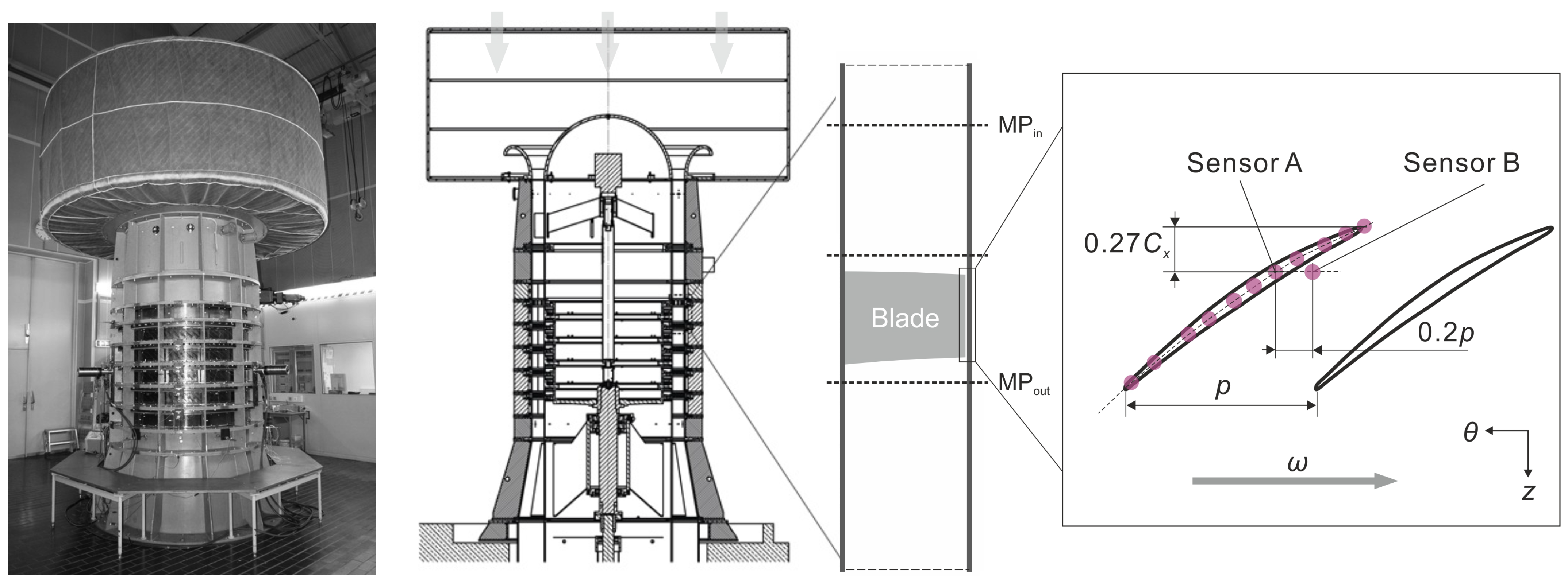
2. Experimental Setup

The investigated object in this paper is a single rotor of the LSRC operated by the Chair of Turbomachinery and Flight Propulsion at Technische Universität Dresden (Figure 1). The compressor is vertically arranged with a downward flow direction. The reference build-up consists of four stages, but for investigating the specific flow features of a rotor blade row, only a single rotor row (without rotor-stator interaction) was retained and experimentally investigated. The inlet flow has no swirl as no inlet guide vane was present. The rotor blade profile, which was designed to model a middle-stage group of a high-pressure compressor, corresponds to the reference build of the compressor as documented by Boos et al. [30]. Time-averaged flow field data were acquired using a cranked five-hole probe with a spherical head of 2 mm diameter up- and downstream of the blade row (MPin and MPout in Figure 1). On the shroud wall, Kulite sensors, with the arrangement demonstrated in Figure 1, were placed along the blade chord direction and at 0.27 axial chord length ( C x ) downstream of the blade leading edge. The specification of the test rig is presented in Table 1. By milling the compressor blades while keeping the casing diameter unchanged, different tip clearances were obtained. The blade tip clearance (s) for the investigated compressor as well as the relative size to the blade tip chord length (C) are shown in Table 2.

3. Numerical and Mathematical Approaches
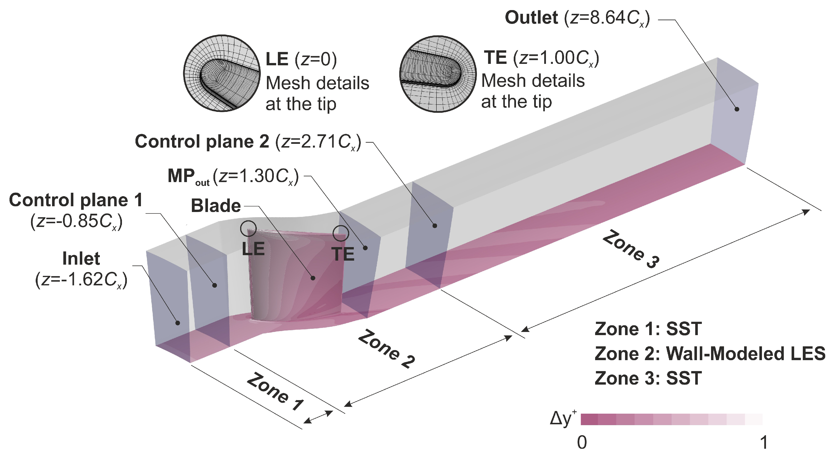
3.1. Mesh Setup

The mesh and the numerical setups in this paper are based on authors’ previous research [29]. The mesh for numerical simulations was generated using NUMECA/AutoGrid5. The computational domain of the research object is presented in Figure 2. Two control planes were set at 0.85 C x upstream of the rotor blade leading edge (LE) and at 1.71 C x downstream of the rotor blade trailing edge (TE), splitting the mesh domain into three zones. Regarding the mesh structures, O4H topology was employed to encircle the rotor blade, and OH topology was used for the blade tip clearance. Blocks with H topology were utilized as the extending segments apart from the blade region, and all the nodes were fully matched between adjacent mesh blocks as well as the periodic boundaries. As for the nodes, 209 grid points were set surrounding the blade circumference, and 161 layers (41 nodes for the tip clearance) were specified in the radial direction. The normalized wall cell dimension normal to the wall fulfills Δ y + < 1 (see contours). Over the whole simulation domain, the minimum skewness of the mesh is 28.7°, and the maximum expansion ratio is 2.8. Finally, 2.39 million nodes (1.97 million nodes in zone 2) were employed for the computational region. Grid validation has been carried out beforehand, and the result implies that the selected mesh setup satisfies the grid independence for simulating the flow features of the investigated compressor.

3.2. Numerical Setup
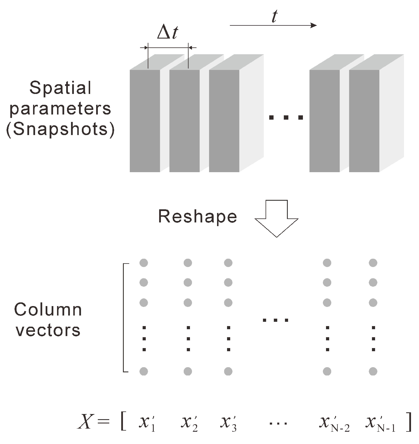
The simulations were performed using ANSYS-CFX 2020 R2. The zonal large eddy simulation (ZLES) model, as a beta function in the current ANSYS-CFX version, was employed as the numerical model [31,32]. In this method, the shear stress transport (SST) model as a Reynolds-averaged Navier–Stokes (RANS) approach was applied in zone 1 and zone 3 as depicted in Figure 2, whereas wall-modeled LES was specified in zone 2 aiming at capturing the complex and turbulent flow characteristics within the blade row. To provide a time-resolved turbulent inlet condition to the LES zone (zone 2), resolved turbulence was artificially generated by a synthetic turbulence generator at the RANS/LES interface. As for the numerical schemes, the high resolution, as a bounded second-order upwind biased discretization, was used as the advection scheme in the SST zones. The bounded central difference scheme was employed for zone 2.
After an independence check, the physical timestep was specified as 4.76 × 10 5 s, corresponding to 5% of the time for the blade passing one blade pitch (T). The inner loops within each physical timestep were selected as 5, and the second-order backward Euler method was chosen as the transient scheme. Absolute total pressure, turbulence kinetic energy, turbulence eddy dissipation, and ambient total temperature obtained from the experiment were imposed at the inlet boundary. The wall boundary was specified as no-slip, smooth and adiabatic.
In addition to the grid size, the number of meshed passages was tested. Three different numerical cases were set up as shown in Table 3. The mesh of the multi-passage configuration was obtained through annular duplication of the single-passage mesh (PSG1). The total grid number for each case is in proportion to the passage number.

3.3. DMD Method

In the post-processing of the simulation results, dynamic mode decomposition (DMD) can be employed for filtering the flow data to specific frequencies and visualizing the temporal-spatial characteristics. The details of the algorithm have been stated in [33]. Here, only a short summary of the method is provided.
The spatial-distributed variables at each CFD timestep define one snapshot. A series of snapshots is collected from the consecutive CFD transient results, and the ensemble-averaged database Ψ 0 is extracted. Once the data are obtained, a pre-processing is performed. The offset snapshots (original values minus Ψ 0 ) x 1 , x 2 , …, x N 1 are collected as sketched at the top of Figure 3. For each snapshot, the data are reshaped into a column vector, and all the snapshots make up the DMD matrix X. Each column in matrix X contains the entries of the spatial flow information at one instant (snapshot), and the time between two adjacent snapshots is Δ t .
Assuming a linear dynamic system for mapping the current flow data to the subsequent flow data, we have:
x i + 1 = A x i ,
where A is the system matrix, and it is assumed to be constant for the entire snapshot sequence.
By applying the similarity transformation, a similarity matrix of A can be obtained as A ˜ . The eigenvalue, the eigenvector, the dynamic mode, and the corresponding mode amplitude are represented as μ j , w j , Ψ j and α j , respectively. The significance of the mode is sequentially ranked by mode amplitude. The reconstructed flow fields x i , r e c by the first r modes reads:
x i , r e c = Ψ 0 + j = 1 r Ψ j ( μ j ) i 1 α j
Using Ψ ˜ j ( t = i ) as a representative of flow field component corresponding to Ψ j at timestep i, the reconstructed flow at timestep i is transformed to:
x r e c ( t = i ) = Ψ 0 + j = 1 r Ψ ˜ j ( t = i )

4. Results and Discussion

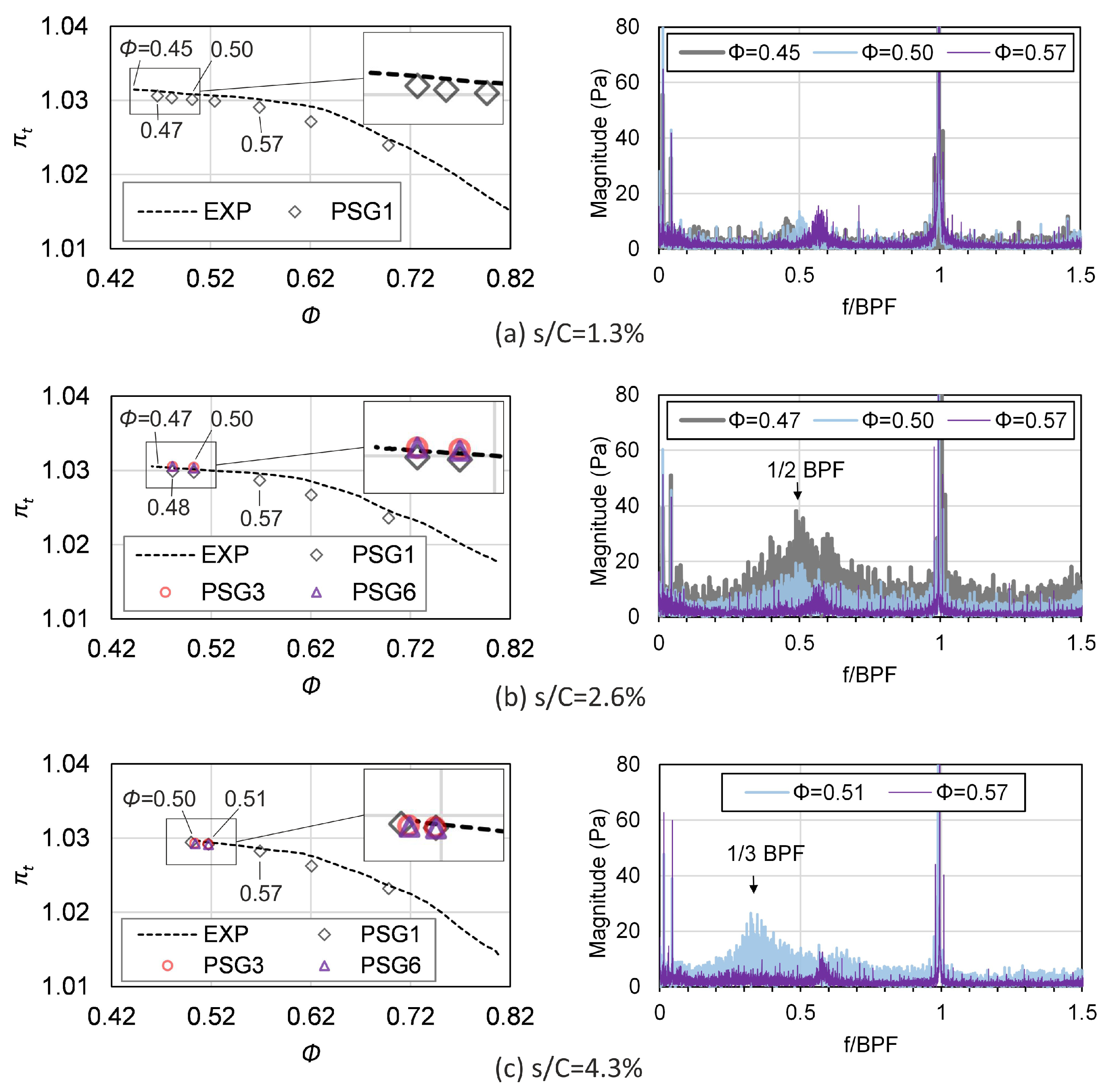
4.1. Overall Performance

Figure 4 shows the speedline of compressor and the fast Fourier transform (FFT) spectra of wall pressure sensor. The speedline of the compressor is characterized by flow coefficient ( Φ ) and total pressure ratio ( π t ). Here, Φ is defined as the ratio of averaged axial velocity at the inlet ( c ¯ a ) to the blade tip speed ( u t ), and π t is the ratio of the averaged total pressure from MPout to MPin. The measured speedline (labeled as EXP) is presented as the dashed line in the left charts, and the FFT spectra of wall pressure measured from the Kulite sensor A (see locations in Figure 1) are illustrated on the right.
As seen in EXP, with the increase of tip clearance, the total pressure ratio sees a slight drop while the stall point shifts to a higher flow coefficient. Regarding the spectra, the variation is hardly visible at different operating points for the small tip clearance ( s / C = 1.3 % ). As the tip gap extends, a hump in the FFT spectra of the throttled operating points becomes prominent, while at the design point ( Φ = 0.57 ), no change is detectable. The frequency of the hump is about 1/2 BPF for s / C = 2.6 % and reduces to around 1/3 BPF for s / C = 4.3 % , which corresponds to the previous observation in the other tests based on the LSRC [2,7]. Such unsteady disturbances indicated by the narrow-band region below the BPF are believed to be the RIs. It should be noted that small humps are seen around 0.5–0.6 BPF for all three cases at Φ = 0.57 . This signal is not related to the rotor tip flow field, and thus it is neglected in the further discussion.
Regarding the CFD results, the speedline was calculated by changing the static pressure at the outlet boundary. A step of 50 Pa was used to obtain the last few stable operating points before stall. The stability limit is well captured by the simulations of the largest tip clearance in Figure 4c, while there is a small deviation for Φ between the predicted results and the measured near stall point for the other two cases. Nevertheless, the trend that reducing tip clearance leads to a larger operating range also applies to the simulation results. For medium and large clearance cases, the near stall points have also been calculated with three and six passages. No influence on the averaged pressure ratio and the stall point is detected, which implies that the number of meshed passages has a limited impact on simulating the averaged characteristics of the investigated compressor.
Radial distributions of relative flow angle ( β ) and circumferential-averaged axial velocity ( c a ), with the latter normalized by c ¯ a , are available from the five-hole probe measurements. The measured data and the predictions are compared in Figure 5. Regardless of the variation of the tip gap, the distributions of β and c a / c ¯ a are well simulated. The remarkable agreement between EXP and the CFD results suggests that the current simulation method is reliable in predicting the averaged flow features. As for the effect of the number of meshed passages, the results illustrate little change, implying that the meshed passage number barely influences the averaged CFD results. Further comparison at the design point and the discussion of the numerical model are provided in [29].

4.2. Dynamic Characteristics

To compare the dynamic behaviour, the wall pressure signals at sensor A and B (locations shown in Figure 1) are collected in the stationary frame in the simulations and processed in comparison to the experimental data. Figure 6 depicts the results for the compressor with the middle tip gap at Φ = 0.50 . The first row shows the FFT spectra of wall pressure presented by power spectral density (PSD). The following rows show the correlated information between the two sets of signals, including squared spectral coherence ( γ x y 2 ), phase angle ( Θ x y ), and sequentially calculated propagation velocity ( c x y ) normalized by the magnitude of the blade tip velocity ( u t ). In the spectra, the positive sign in Θ x y and propagation velocity corresponds to the direction of the blade rotation.
For the measured data shown in Figure 6d, the characterized frequency of RIs is close to 1/2 BPF. Meanwhile, the simulations capture the hump of RI in all the numerical cases regardless of the number of passages, although the distribution of the spectrum varies in each case. Significant correlations are found near the frequency of 1/2 BPF for PSG1 and PSG3, while, for PSG6 and the experimental data, the correlation is less clear but still increased compared to the surrounding frequency band. The propagation velocity of the perturbation is calculated as half of the rotor speed ( c x y / u t = 1 / 2 ) from the view of the stationary reference. In the rotating frame, the corresponding velocity can be calculated as half of the rotor speed while in a reversed direction. Since the change of reference frame does not influence the wavelength, the frequency of the dominant perturbation is calculated as 1/2 BPF, which is identical to the value shown in the stationary frame.
Unlike the scenario for the configuration with a middle tip gap, the prediction of the dominant frequency below the BPF is case-dependent when the tip gap increases to s / C = 4.3 % . In Figure 7a, high magnitudes are observed within a narrow band near 1/2 BPF, which deviates from the experimental result (EXP) where the dominant frequency is located near 1/3 BPF. Once the number of meshed passages increases to 3 (Figure 7b), the low-frequency hump shifts to 1/3 BPF and coincides with the frequency of the RI in EXP. As for PSG6 presented in Figure 7c, the spectrum shows a similar distribution as PSG3, and the characterized low-frequency disturbance lies around 1/3 BPF.
Apart from a high correlation at BPF, γ x y 2 owns a high value at the featured frequency as highlighted in the first row, showing the signals from two sensors are strongly related. Regarding the phase angle shown in the third row, the distributions of Θ x y near 1/3 BPF present nearly identical trends. The calculated propagation velocity of the perturbation at 1/3 BPF is around half of the blade rotating speed if considered in the stationary reference frame. Using the same method as described above, the arithmetic results indicate that the RI presented in the rotating frame has a frequency of 1/3 BPF and owns a reversed direction of the blade rotating and half of the rotor speed.
Although the frequency of RI is captured in PSG3 and PSG6, it should be noticed that the bandwidth of the bump in simulations is narrower than EXP, which may result from the fact that the simulations are not able to capture adequate modes due to the limited number of passages. For both cases, PSG6 shows additional peaks in the spectra and high correlation values next to the primarily investigated frequency, which can be seen as modulation of the RI. Nevertheless, PSG6 captures the characterized dynamics and is finally selected as the numerical object. The discussions on the simulations are based on PSG6 throughout the following context.
By processing the experimental data from the sensors arranged along the blade chord, the PSD of wall pressure at different axial locations is depicted in Figure 8, where z / C x = 0 corresponds to the LE and z / C x = 1 stands for the TE. For s / C = 2.6 % , the band of RIs with 1/2 BPF is significant along the axial direction. The amplitude increases slightly from the LE and reaches the maximum near 0.3 C x . In comparison, the RI shown in Figure 8b can be viewed as a ridge located at 1/3 BPF. The RI signal at the LE is relatively weak, while it gets intensive and reaches the highest PSD value near 0.4 C x .
Figure 9 demonstrates the simulated flow features near the blade tip region. At the lower part of the figure, the distributions of standard deviation (STD) of wall pressure ( σ p ) normalized by atmosphere pressure ( p a t m ) and the contour lines of pressure are presented. The trajectory of the tip leakage vortex (TLV) is marked by the dashed lines. For the upper part, the streamlines are colored by the velocity magnitude ( c x y z ) normalized by u t .
For both tip clearance sizes shown in Figure 9, the TLV crosses the passage from its originating blade and extends towards the pressure side of the adjacent blade. There, a significant part of the vortex flow travels over the blade tip and contributes to the formation of the TLV in the following passage. The trajectory is marked by an increased normalized σ p , where the higher values tend to be on the upstream side of the vortex core. Near the pressure side of the adjacent blade, the peak of σ p is seen, indicating the high flow fluctuations in this region. As the TLV shows a steeper trajectory for the middle tip gap case (see Figure 9a), the area of high fluctuations is located closer to the LE. In contrast, the high σ p values can be found further towards mid-chord and with an increased affected area when the blade tip clearance is large. The location with the highest σ p corresponds to the detected dominant RI signal as shown in Figure 8, which implies that the RI can be correlated to the perturbation of blade tip flow for this test case.

4.3. DMD-Based Analysis

Based on the discussion in the above sections, some dynamic properties of RI are explored. However, the physical interpretation of the RI is unclear and remains to be further elucidated. Since the ZLES model was applied for simulations, the CFD results are relatively noisy. A large variety of irregular vortices is seen in the CFD post-processing of the instantaneous solutions, and coherent flow structures can hardly be observed or classified into certain frequencies intuitively. Considering this issue, the data-driven method DMD was employed to the CFD snapshots, and the filtered flow field with a single frequency was specifically extracted.
Among the transient numerical results (presented in the rotating frame of reference), the three-dimensional pressure field over the blade row at one CFD timestep was selected as a snapshot. Independence validation on the number of snapshots was performed beforehand, and 1000 snapshots were finally collected as the database, which corresponds to the physical time for the blade passing 100 pitches.
The normalized DMD amplitude | α n o r m | assesses the significance of a mode over the dynamic evolution. As presented in Figure 10, modes with high | α n o r m | are sparsely distributed and a dominant frequency is detected in each case. The highest | α n o r m | is seen at 1/2 BPF for s / C = 2.6 % and at 1/3 BPF for s / C = 4.3 % (marked by circles). The featured frequencies are identical to the expected dominant RI frequencies as concluded in Figure 6 and Figure 7, suggesting that the DMD algorithm successfully identifies the desired RI dynamics.
In Figure 11, the top-ranked mode is visualized by the iso-surfaces of the non-dimensional pressure, which reflects the status of pressure fluctuation (i.e., a positive value means local expansion while a negative value stands for local contraction). The mode is observed as the wave whose troughs and crests are staggered with the blade. Furthermore, the wave is located near the tip region, suggesting that the perturbation is a consequence of the unsteady behavior of the tip flow. For s / c = 2.6 % , the spatial wavelength in the circumferential direction equals one pitch (p), whereas the wave has an annular wavelength of 1.5 p when s / C = 4.3 % .
Figure 12 demonstrates the ensemble-averaged pressure ( ψ 0 ), the evolution of the pressure ( ψ ˜ 1 ) corresponding to top-ranked mode, and the reconstructed flow ( ψ 0 + ψ ˜ 1 ) at one timestep at 95 % span. To evaluate the change in the local pressure difference driving the tip leakage flow, the normalized pressure difference ( Δ p n o r m ) between the pressure and suction sides of blade B4 normal to the chord is presented at the bottom correspondingly (LE locates at 0 while TE is at 1). The time for the blade passing one blade pitch is labeled as T. It should be noted that all the figures are spatially depicted in the rotating frame of reference.
For the averaged flow field ψ 0 , no change from passage to passage, as expected, is seen. The local maximum pressure difference is at 20% chord apart from the peak near LE.
Taking the highlighted B4 as an example. At t = 0 , a low-pressure spot (marked by a dashed rectangular frame) is approaching the LE, and the pressure difference reaches the minimum value. The reducing Δ p n o r m results in a degradation of the tip leakage flow near the LE, as the driving force for the blade tip leakage is reduced. Therefore, a high-pressure spot, which represents a weakened TLV, gradually emerges over the suction side of B4 as shown at t = 4 / 10 T . Meanwhile, the same topology can be found near the suction side of B3. With time varying, the low-pressure spot propagates downstream along the pressure side and the LE of B4 starts to experience the high-pressure spot from the suction side of B3. As a result, pressure difference increases at the LE and turns to a positive value at t = 8 / 10 T . The rising Δ p n o r m provides the potentials to generate a more intensive TLV until 12 / 10 T , at which the pressure difference becomes maximum because the high-pressure spot reaches the pressure side. The strong TLV is represented by the low-pressure spot originating from the LE. It develops into the passage and then approaches the blade pressure side near the LE, leading to a drop for the pressure difference and finally a repeated scenario as t = 0 at t = 20 / 10 T .
The low-pressure spots propagate synchronously (in the same phase) in the neighboring passages, which ultimately forms a wave trough indicated by a low-pressure strip (shaded by a window). As shown by the evolution of the highlighted window, the wave travels downstream at a constant speed. Once the time passes 2 T , the same topology is detected at the same location, suggesting that the wave has a period of 2 T . The wavelength projected to the circumferential direction is 1 p , thus the propagation velocity is p / 2 T with a reversed direction as the rotor. One instantaneous reconstructed flow ( ψ 0 + ψ ˜ 1 ) is also illustrated. The least common multiple of the wavelength in ψ ˜ 1 , and the blade passage size equals 1 p in the pitchwise direction. Therefore, the reconstructed flow shares the same topology in different passages.
Concerning the configuration with large tip clearance, the ensemble-averaged pressure ( ψ 0 ) and the DMD results at one timestep are presented in Figure 13. The dynamic properties vary, as the tip gap increases from 2.6%C to 4.3%C.
According to the averaged flow field ψ 0 , the flow patterns are the same in different passages. However, the trajectory of the TLV is deviated from the distribution for the configuration with a middle tip gap. The TLV trace shifts to the mid-chord region, and the location for the local maximum pressure difference moves downstream.
Blade B4 is selected as an example again. A low-pressure zone (marked by a dashed rectangular frame) is approaching the LE at t = 0 T . The minimum Δ p n o r m drops to −0.004, which is near twice the magnitude for the middle tip gap configuration. The low Δ p n o r m results in a weak TLV, thus a high-pressure spot near the suction side of B4 starts to form. In contrast to the symmetrical patterns in different passages, the flow topologies depicted in Figure 13 are no longer the same in the neighbouring passages, and the pressure spots (both high and low) impose long-lasting influence over the flow evolution. Along the pressure side of B4, the low-pressure spot travels downstream. Gradually, the influence of the weak TLV (high-pressure zone) from B3 approaches the LE of B4 at t = 18 / 10 T , and Δ p n o r m reaches the maximum value of 0.004. Sequentially, an intensive TLV emerges from the LE of B4, and the wake spreads to the adjacent blade. Meanwhile, the high-pressure and low-pressure zones keep moving downstream along the pressure side of B4. At t = 30 / 10 T , the LE of B4 finally experiences the low pressure from the downstream influence of the intensive TLV of B3. The pressure difference Δ p n o r m drops to the minimum value like the initial timestep t = 0 , forming a repetition with a period of 3 T .
Regarding the flow patterns in adjacent passages, the synchronous propagation of the low-pressure region (shaded by a window) can be observed as a wave trough. The wavelength projected to the pitchwise direction is equal to 1.5 p . When the wavelength is divided by the time period of 3 T , the propagation velocity in the rotating frame is equal to the middle tip clearance case at p / 2 T in a reversed direction of the blade rotation.
Based on the above discussion, a sketch is proposed to explain the mechanism of RIs in Figure 14. As a bulk of the TLV stretches to the front part of the adjacent blade, the pressure distribution over the blade is affected and the unsteady behaviors of the tip leakage flow are triggered. The unsteady behaviors of tip leakage flow are presented as pressure waves form, which is essentially equivalent to RI. The tip leakage flow determines the wave (RI) properties, which own various frequencies with a dominant one always detected. The pressure wave travels and influences the pressure distribution over the blade tip region. Consequentially, the pressure difference is affected, modifying the tip leakage flow and forming the RI-mechanism loop at the end. Over time, the TLV-trajectory presents a periodically flapping motion, which substantiates the theory proposed by Mailach et al. based on experiments of an axial compressor [2] and a linear cascade [6]. To change the RI properties or cushion the RI influence, flow control methods can be proposed by interfering steps in the loop based on Figure 14.
In comparison to other studies in literature for the current test case, no signs were found regarding the backflow around the TE with impingement on the pressure side as detected by Vo [18], nor did the purely data driven method of DMD detect any coherence of the inlet boundary layer to the RI frequency as proposed by Pardowitz et al. [21,22,23]. Furthermore, as a stable operating point close to the stability limit was investigated, the fluctuations of the leakage vortex are periodic, and no indications of the development of tornado-like vortices close to the LE [34,35] are found.

5. Conclusions

In this paper, a single compressor rotor row at varying blade tip clearances ( s / C = 1.3 % , 2.6 % , and 4.3 % ) is selected as the research object. The compressor was simulated using the ZLES model. The properties and the mechanism of RIs are analyzed, and some conclusions can be drawn as follows:
As the compressor is throttled to the near stall operating point, the experimental data indicate that the amplitude in a low-frequency band becomes significant for the configurations with middle and large tip gaps ( s / C = 2.6 % and 4.3 % ), suggesting that the RIs are observed. The characterized frequency is 1/2 BPF for the former while 1/3 BPF for the latter. The propagation velocity of RIs is equal to half of the rotor speed if observed in the stationary frame.
In simulations, the number of the meshed passages has a limited influence on predicting the averaged flow parameters but determines the properties of pre-stall dynamic features like RI. Near the stability limit of the compressor, the numerical results present remarkable behavior in capturing the radial distributions of the circumferential-averaged profiles, and the mesh with six meshed passages is proved to be reasonable in capturing the characterized RI properties.
For the configurations with middle and large tip clearances, the DMD approach successfully extracts the dominant dynamics. The corresponding modes are visualized as the waves located near the blade tip region and staggered with the blade. The analysis of the DMD results indicates that the RI is essentially the pressure wave traveling over the blade tip region. The azimuthal wavelength is 1 p for s / C = 2.6 % while 1.5 p for s / C = 4.3 % . The simulated traveling velocity of RI agrees well with the experimental measurements.
RIs are essentially equivalent to the waves which are composed of multiple frequencies and propagate over the blade tip. In the blade tip region, the TLV stretches to the front part of the adjacent blade, which correspondingly affects the pressure distribution and triggers unsteady behaviors of the tip leakage flow. The unsteady behaviors of tip leakage flow are presented as pressure waves with specific dynamic properties. The pressure wave travels over the blade tip region and alters the pressure distribution. As a result, the pressure distribution changes, which, in turn, determines the tip leakage flow. A periodic loop is established at the end.
To vary the RI properties, flow control methods are suggested to be leveraged via modifying any steps in the RI-mechanism loop proposed in this paper.

Author Contributions

Conceptualization, X.C., B.K., M.L. and R.M.; methodology, X.C.; software, X.C.; writing—original draft preparation, X.C.; writing—review and editing, X.C., B.K., M.L., W.C. and R.M.; visualization, X.C.; supervision, W.C. and R.M. All authors have read and agreed to the published version of the manuscript.

Funding

The research was conducted as part of the joint Ph.D. program between Northwestern Polytechnical University and Technische Universität Dresden (TU Dresden) funded by the China Scholarship Council (CSC) under Grant No. 201906290098. The research was also funded and supported by the Deutsche Forschungsgemeinschaft (DFG) under Grant No. MA4922/8-1 as part of the package proposal PAK948. The experimental results were obtained within the framework of the joint project “Flow in the endwall region of turbomachinery blading”.

Acknowledgments

The authors gratefully acknowledge the computational resources provided by the Bull High Performance Computing at the Center for Information Services and High Performance Computing at TU Dresden.

Conflicts of Interest

The authors declare no conflict of interest.

Abbreviations

The following abbreviations are used in this manuscript:
BPFBlade passing frequency
CFDComputational fluid dynamics
DMDDynamic mode decomposition
FFTFast Fourier transform
LELeading edge
LSRCLow speed research compressor
NSVNon-synchronous vibration
PSDPower spectral density
RANSReynolds-averaged Navier–Stokes
RIRotating instability
SSTShear stress transport
STDStandard deviation
TETrailing edge
TLVTip leakage vortex
ZLESZonal large eddy simulation

References

  1. Day, I.J. Stall, Surge, and 75 Years of Research. J. Turbomach. 2015, 138, 011001. [Google Scholar] [CrossRef]
  2. Mailach, R.; Lehmann, I.; Vogeler, K. Rotating Instabilities in an Axial Compressor Originating from the Fluctuating Blade Tip Vortex. J. Turbomach. 2000, 123, 453–460. [Google Scholar] [CrossRef]
  3. Mathioudakis, K.; Breugelmans, F.A.E. Development of Small Rotating Stall in a Single Stage Axial Compressor. In Volume 1: Aircraft Engine; Marine; Turbomachinery; Microturbines and Small Turbomachinery; V001T03A064; Turbo Expo: Power for Land, Sea, and Air; American Society of Mechanical Engineers: New York, NY, USA, 1985. [Google Scholar] [CrossRef] [Green Version]
  4. Liu, J.; Holste, F.; Neise, W. On the azimuthal mode structure of rotating blade flow instabilities in axial turbomachines. In Proceedings of the Aeroacoustics Conference, State College, PA, USA, 6–8 May 1996; American Institute of Aeronautics and Astronautics: Reston, VA, USA, 1996. [Google Scholar] [CrossRef]
  5. Kameier, F.; Neise, W. Experimental Study of Tip Clearance Losses and Noise in Axial Turbomachines and Their Reduction. J. Turbomach. 1997, 119, 460–471. [Google Scholar] [CrossRef]
  6. Mailach, R.; Sauer, H.; Vogeler, K. The Periodical Interaction of the Tip Clearance Flow in the Blade Rows of Axial Compressors. In Volume 1: Aircraft Engine; Marine; Turbomachinery; Microturbines and Small Turbomachinery; American Society of Mechanical Engineers: New York, NY, USA, 2001. [Google Scholar] [CrossRef]
  7. Rolfes, M.; Lange, M.; Mailach, R. Investigation of Performance and Rotor Tip Flow Field in a Low Speed Research Compressor with Circumferential Groove Casing Treatment at Varying Tip Clearance. Int. J. Rotating Mach. 2017, 2017, 4631751. [Google Scholar] [CrossRef] [Green Version]
  8. Beselt, C.; van Rennings, R.; Sorge, R.; Peitsch, D.; Thiele, F.; Ehrenfried, K.; Thamsen, P.U.; Pardowitz, B.; Enghardt, L. Influence of the clearance size on rotating instability in an axial compressor stator. In Proceedings of the 10th European Conference on Turbomachinery Fluid dynamics & Thermodynamics, Lappeenranta, Finland, 15–19 April 2013; European Turbomachinery Society: Florence, Italy, 2013. [Google Scholar]
  9. Wu, Y.; Wu, J.; Zhang, G.; Chu, W. Experimental and Numerical Investigation of Flow Characteristics Near Casing in an Axial Flow Compressor Rotor at Stable and Stall Inception Conditions. J. Fluids Eng. 2014, 136, 111106. [Google Scholar] [CrossRef]
  10. Yang, W.; Wang, Y.; Han, L.; Zhang, X.; Li, Z. Effect of Rotating Instabilities on Aerodynamic Damping of Axial Flow Fan Blades. In Volume 7A: Structures and Dynamics; American Society of Mechanical Engineers: New York, NY, USA, 2019. [Google Scholar] [CrossRef]
  11. Biela, C.; Müller, M.W.; Schiffer, H.P.; Zscherp, C. Unsteady Pressure Measurement in a Single Stage Axial Transonic Compressor near the Stability Limit. In Volume 6: Turbomachinery, Parts A, B, and C; American Society of Mechanical Engineers: New York, NY, USA, 2008. [Google Scholar] [CrossRef]
  12. Hah, C.; Bergner, J.; Schiffer, H.P. Tip Clearance Vortex Oscillation, Vortex Shedding and Rotating Instabilities in an Axial Transonic Compressor Rotor. In Volume 6: Turbomachinery, Parts A, B, and C; American Society of Mechanical Engineers: New York, NY, USA, 2008. [Google Scholar] [CrossRef]
  13. Sun, Z.; Zou, W.; Zheng, X. Instability detection of centrifugal compressors by means of acoustic measurements. Aerosp. Sci. Technol. 2018, 82–83, 628–635. [Google Scholar] [CrossRef]
  14. He, X.; Zheng, X. Roles and mechanisms of casing treatment on different scales of flow instability in high pressure ratio centrifugal compressors. Aerosp. Sci. Technol. 2019, 84, 734–746. [Google Scholar] [CrossRef]
  15. Zhang, L.Y.; He, L.; Stüer, H. A Numerical Investigation of Rotating Instability in Steam Turbine Last Stage. J. Turbomach. 2012, 135, 011009. [Google Scholar] [CrossRef]
  16. Gerschütz, W.; Casey, M.; Truckenmüller, F. Experimental investigations of rotating flow instabilities in the last stage of a low-pressure model steam turbine during windage. Proc. Inst. Mech. Eng. Part A J. Power Energy 2005, 219, 499–510. [Google Scholar] [CrossRef]
  17. Hoying, D.A.; Tan, C.S.; Vo, H.D.; Greitzer, E.M. Role of Blade Passage Flow Structurs in Axial Compressor Rotating Stall Inception. J. Turbomach. 1999, 121, 735–742. [Google Scholar] [CrossRef]
  18. Vo, H.D. Role of Tip Clearance Flow in Rotating Instabilities and Nonsynchronous Vibrations. J. Propuls. Power 2010, 26, 556–561. [Google Scholar] [CrossRef]
  19. März, J.; Hah, C.; Neise, W. An Experimental and Numerical Investigation into the Mechanisms of Rotating Instability. J. Turbomach. 2002, 124, 367–374. [Google Scholar] [CrossRef]
  20. Kielb, R.E.; Barter, J.W.; Thomas, J.P.; Hall, K.C. Blade Excitation by Aerodynamic Instabilities: A Compressor Blade Study. In Proceedings of the Turbo Expo 2003, Atlanta, GA, USA, 16–19 June 2003; American Society of Mechanical Engineers: New York, NY, USA, 2003; Volume 4. [Google Scholar] [CrossRef] [Green Version]
  21. Pardowitz, B.; Tapken, U.; Enghardt, L. Time-resolved Rotating Instability Waves in an annular Cascade. In Proceedings of the 18th AIAA/CEAS Aeroacoustics Conference (33rd AIAA Aeroacoustics Conference), Colorado Springs, CO, USA, 4–6 June 2012; American Institute of Aeronautics and Astronautics: Reston, VA, USA, 2012. [Google Scholar] [CrossRef]
  22. Pardowitz, B.; Tapken, U.; Sorge, R.; Thamsen, P.U.; Enghardt, L. Rotating Instability in an Annular Cascade: Detailed Analysis of the Instationary Flow Phenomena. J. Turbomach. 2013, 136, 061017. [Google Scholar] [CrossRef]
  23. Pardowitz, B.; Moreau, A.; Tapken, U.; Enghardt, L. Experimental identification of rotating instability of an axial fan with shrouded rotor. Proc. Inst. Mech. Eng. Part A J. Power Energy 2015, 229, 520–528. [Google Scholar] [CrossRef]
  24. Wu, Y.; Chen, Z.; An, G.; Liu, J.; Yang, G. Origins and Structure of Rotating Instability: Part 1—Experimental and Numerical Observations in a Subsonic Axial Compressor Rotor. In Volume 2D: Turbomachinery; American Society of Mechanical Engineers: New York, NY, USA, 2016. [Google Scholar] [CrossRef]
  25. Geng, S.; Lin, F.; Chen, J.; Nie, C. Evolution of unsteady flow near rotor tip during stall inception. J. Therm. Sci. 2011, 20, 294–303. [Google Scholar] [CrossRef]
  26. Cravero, C.; Marsano, D. Criteria for the Stability Limit Prediction of High Speed Centrifugal Compressors with Vaneless Diffuser: Part I—Flow Structure Analysis. In Volume 2E: Turbomachinery; V02ET39A013; Turbo Expo: Power for Land, Sea, and Air; American Society of Mechanical Engineers: New York, NY, USA, 2020. [Google Scholar] [CrossRef]
  27. Eck, M.; Geist, S.; Peitsch, D. Physics of Prestall Propagating Disturbances in Axial Compressors and Their Potential as a Stall Warning Indicator. Appl. Sci. 2017, 7, 285. [Google Scholar] [CrossRef] [Green Version]
  28. Wang, H.; Wu, Y.; Wang, Y.; Deng, S. Evolution of the flow instabilities in an axial compressor rotor with large tip clearance: An experimental and URANS study. Aerosp. Sci. Technol. 2020, 96, 105557. [Google Scholar] [CrossRef]
  29. Chen, X.; Koppe, B.; Lange, M.; Chu, W.; Mailach, R. Comparison of Turbulence Modeling for a Compressor Rotor at Different Tip Clearances. AIAA J. 2021. [Google Scholar] [CrossRef]
  30. Boos, P.; Möckel, H.; Henne, J.M.; Selmeier, R. Flow Measurement in a Multistage Large Scale Low Speed Axial Flow Research Compressor. In Volume 1: Turbomachinery; American Society of Mechanical Engineers: New York, NY, USA, 1998. [Google Scholar] [CrossRef] [Green Version]
  31. ANSYS CFX. ANSYS CFX-Solver Theory Guide; ANSYS CFX Release 2020; ANSYS: Canonsburg, PA, USA, 2020. [Google Scholar]
  32. Menter, F.R. Best Practice: Scale-Resolving Simulations in ANSYS CFD; ANSYS Germany GmbH: Otterfing, Germany, 2012; Volume 1. [Google Scholar]
  33. Tu, J.H.; Rowley, C.W.; Luchtenburg, D.M.; Brunton, S.L.; Kutz, J.N. On dynamic mode decomposition: Theory and applications. J. Comput. Dyn. 2014, 1, 391–421. [Google Scholar] [CrossRef] [Green Version]
  34. Yamada, K.; Kikuta, H.; Iwakiri, K.I.; Furukawa, M.; Gunjishima, S. An Explanation for Flow Features of Spike-Type Stall Inception in an Axial Compressor Rotor. J. Turbomach. 2012, 135, 021023. [Google Scholar] [CrossRef]
  35. Pullan, G.; Young, A.M.; Day, I.J.; Greitzer, E.M.; Spakovszky, Z.S. Origins and Structure of Spike-Type Rotating Stall. J. Turbomach. 2015, 137, 051007. [Google Scholar] [CrossRef]
Figure 1. Investigated single rotor build-up of LSRC and arrangement of Kulite sensors on the wall.
Energies 14 08369 g001
Figure 2. Computational domain for the single passage.
Energies 14 08369 g002
Figure 3. Pre-processing of data before applying DMD.
Energies 14 08369 g003
Figure 4. Compressor characteristics and experimental FFT spectra of wall pressure for sensor A.
Energies 14 08369 g004
Figure 5. Radial distributions of circumferential-averaged flow parameters at MPout ( Φ = 0.50 for s / C = 1.3 % and 2.6 % ; Φ = 0.51 for s / C = 4.3 % ).
Energies 14 08369 g005
Figure 6. Spectral analysis of the wall pressure in the stationary reference frame for s / C = 2.6 % at Φ = 0.50 .
Energies 14 08369 g006
Figure 7. Spectral analysis of the wall pressure in the stationary reference frame for s / C = 4.3 % at Φ = 0.51 .
Energies 14 08369 g007
Figure 8. PSD of wall pressure at various axial positions in EXP ( s / C = 2.6 % at Φ = 0.50 ; s / C = 4.3 % at Φ = 0.51 ; presented in the stationary frame; dots on z-axis and solid lines corresponding to locations of Kulite sensors).
Energies 14 08369 g008
Figure 9. Normalized standard deviation of wall pressure and normalized velocity distribution of ensemble-averaged tip leakage flow in CFD results ( s / C = 2.6 % at Φ = 0.50 ; s / C = 4.3 % at Φ = 0.51 , presented in the rotating frame).
Energies 14 08369 g009
Figure 10. DMD spectra ( s / C = 2.6 % at Φ = 0.50 ; s / C = 4.3 % at Φ = 0.51 ).
Energies 14 08369 g010
Figure 11. Visualization of top-ranked DMD modes ( s / C = 2.6 % at Φ = 0.50 ; s / C = 4.3 % at Φ = 0.51 ).
Energies 14 08369 g011
Figure 12. Ensemble-averaged pressure, temporal evolution of dominating mode, example of reconstructed pressure, and profile of blade pressure difference at 95 % span for s / C = 2.6 % at Φ = 0.50 .
Energies 14 08369 g012
Figure 13. Ensemble-averaged pressure, temporal evolution of dominating mode, example of reconstructed pressure, and profile of blade pressure difference at 95 % span for s / C = 4.3 % at Φ = 0.51 .
Energies 14 08369 g013
Figure 14. RI-mechanism loop.
Energies 14 08369 g014
Table 1. Parameters for the single rotor test build of LSRC.
CharacteristicValue
Rotating speed1000 rpm
Casing diameter1500 mm
Hub-to-tip ratio0.84
Rotor blade count63
Rotor blade chord length (Tip)116 mm
Solidity of rotor blades (Tip)1.55
Mass flow at design point27.89 kg/s
Reynolds number at rotor inlet (Mid-span, design point) 6.2 × 10 5
Mach number at rotor inlet (Mid-span)0.24
Table 2. Summary of blade tip clearance.
Configurations (mm) s / C (%)
Small1.51.3
Middle3.02.6
Large5.04.3
Table 3. Mesh setup of different numerical cases.
CaseNumber of Meshed PassagesTotal Grid Number (Million)
PSG112.39
PSG337.17
PSG6614.34
Publisher’s Note: MDPI stays neutral with regard to jurisdictional claims in published maps and institutional affiliations.

