
Optimization of Sizing and Operation Strategy of Distributed Generation System Based on a Gas Turbine and Renewable Energy


Abstract
:1. Introduction
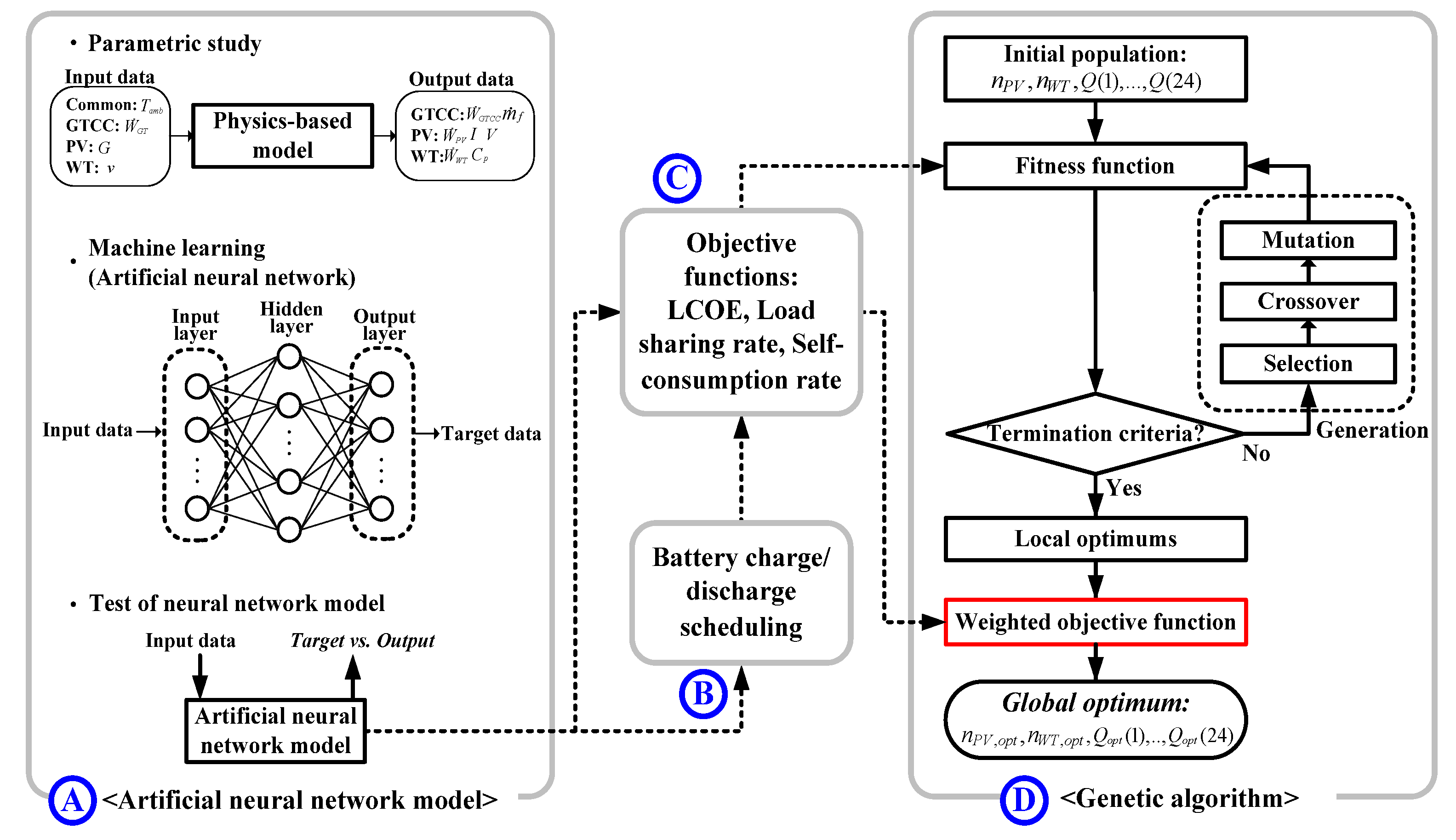
- An artificial intelligence technique that combines an ANN and GA is applied for the complete and robust optimization of the sizing and operation strategy of a DG system.
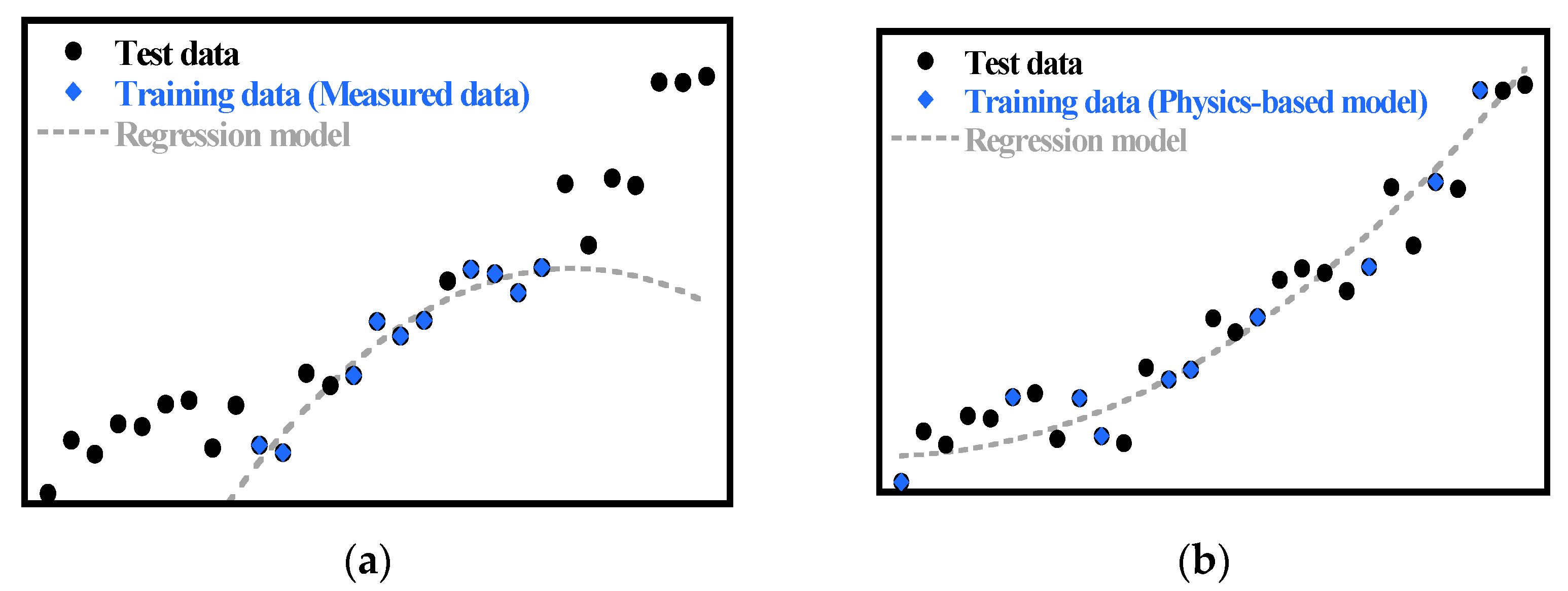
- The ANN is introduced to simulate the physics-based model that can describe the real operating characteristics of every component and improve the computational efficiency.
- Optimization of the sizing and operation strategy of the DG system was performed in consideration of the cost-effectiveness and eco-friendliness.
2. System and Modeling
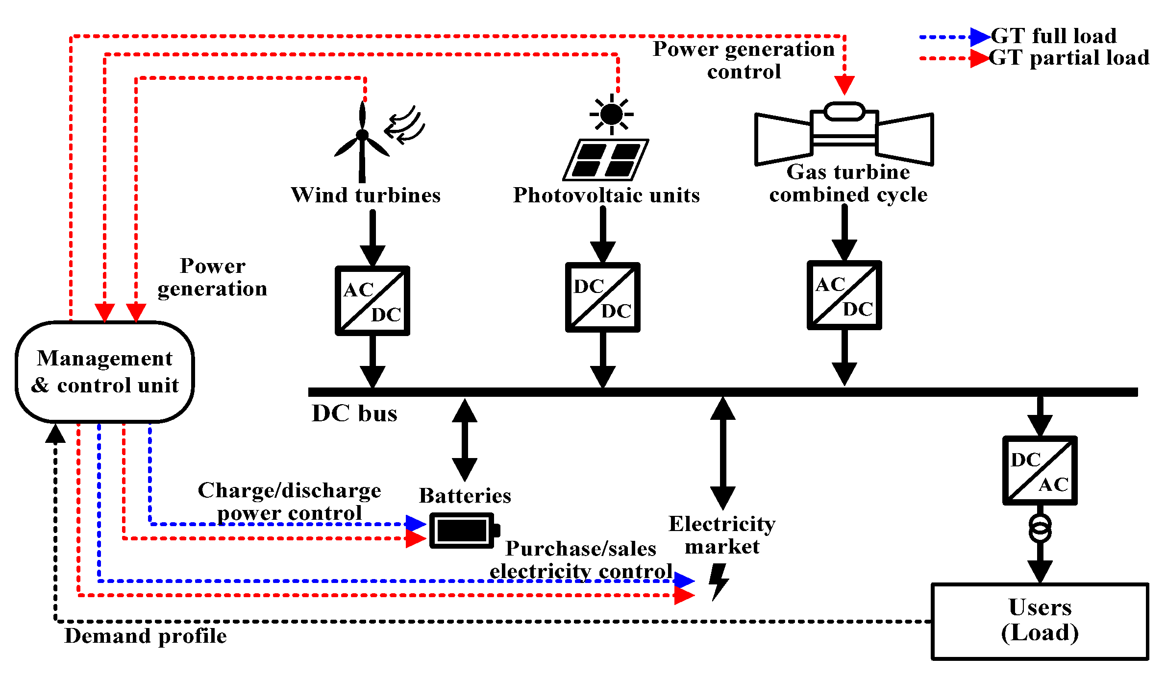
2.1. System Description
2.2. Gas Turbine Combined Cycle
2.2.1. Gas Turbine
2.2.2. Bottoming Cycle
2.3. Renewable Energy
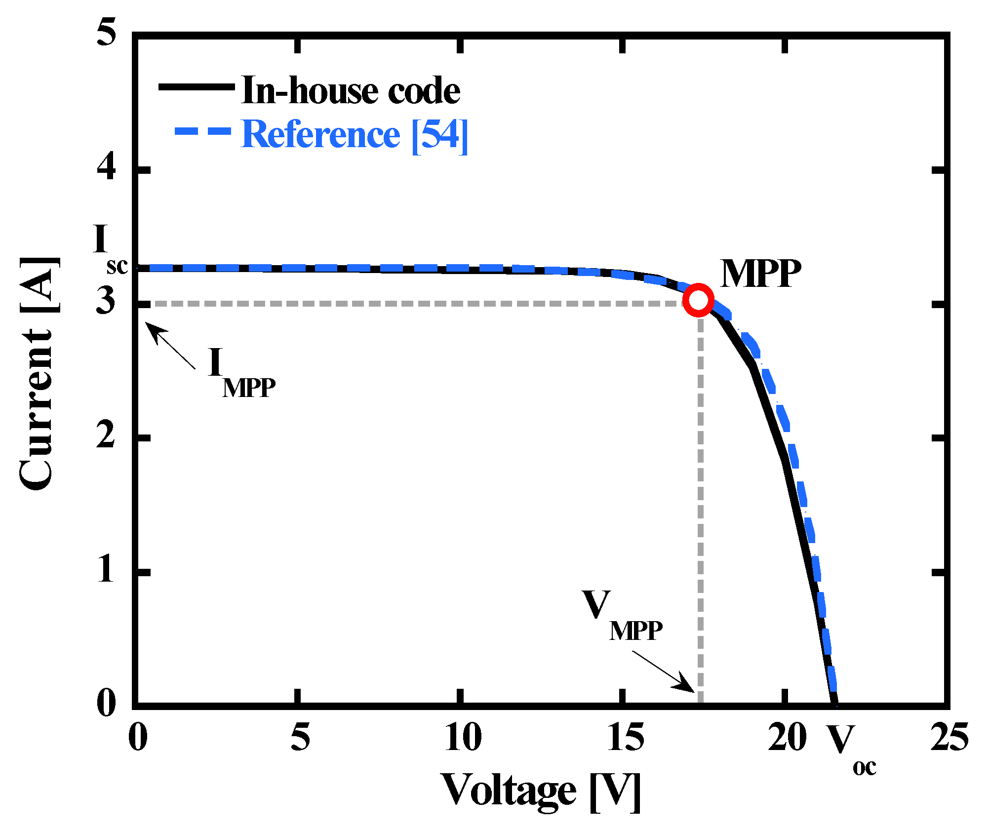
2.3.1. Photovoltaics
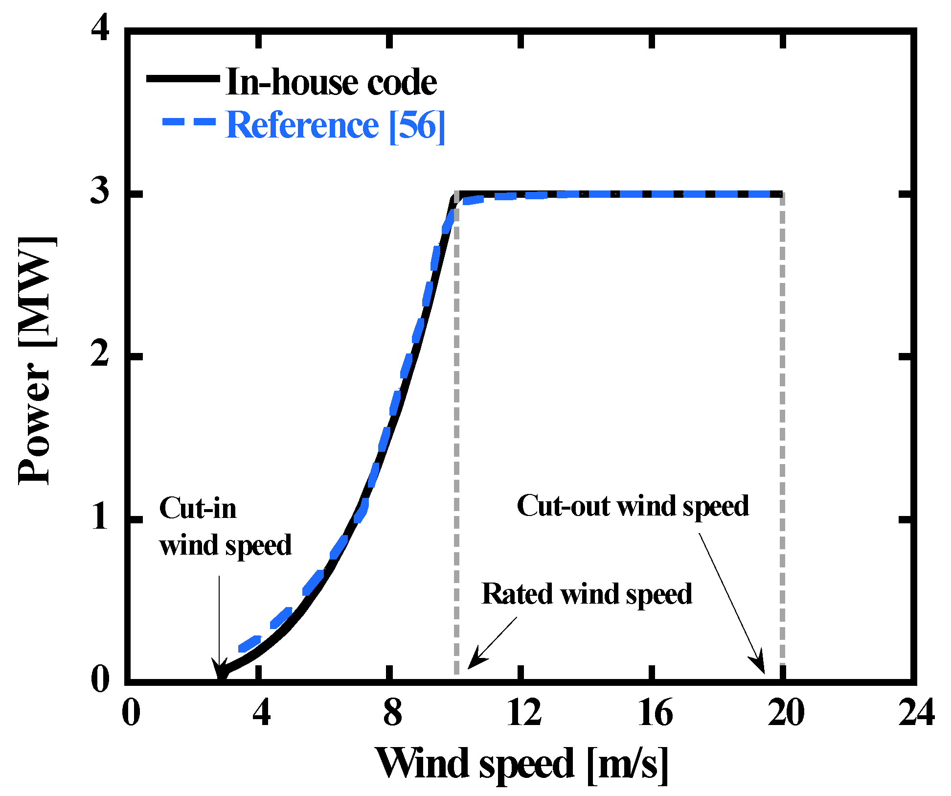
2.3.2. Wind Turbine
2.4. Battery Energy Storage System
3. Analysis and Optimization
3.1. Overview
- Case 1: 15-MW GT, full load operation
- Case 2: 15-MW GT, partial load operation (down to 50% power)
- Case 3: 5.7-MW GT, full load operation
3.2. Artificial Neural Network Model
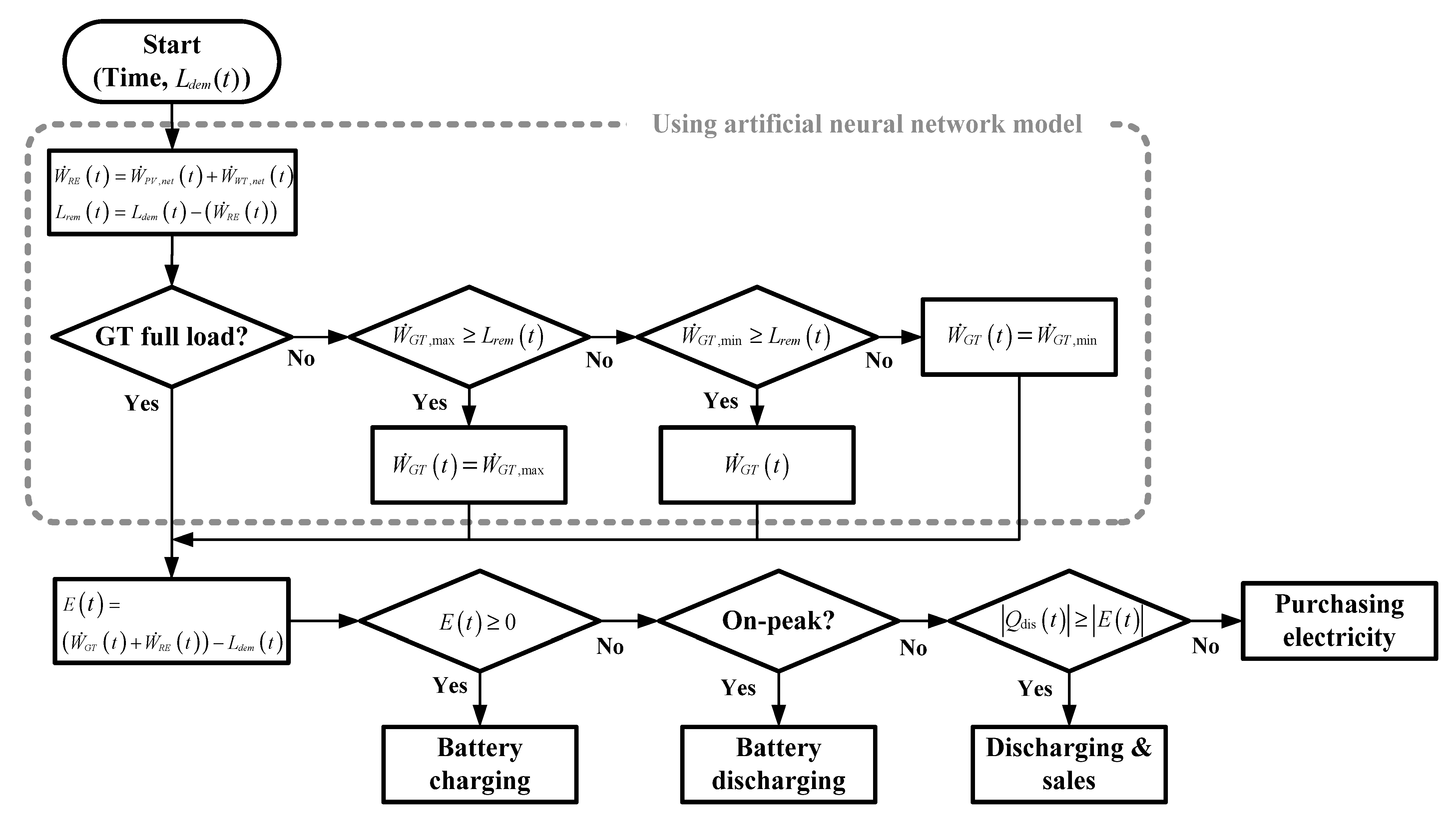
3.3. Battery Charge/Discharge Scheduling
3.4. Objective Functions for Optimization
3.5. Genetic Algorithm
- Maximize the weighted objective function (Equation (31)) subject to
- Design variables:
4. Results and Discussion
4.1. Performance of the ANN Model
4.2. Optimization Results
5. Conclusions
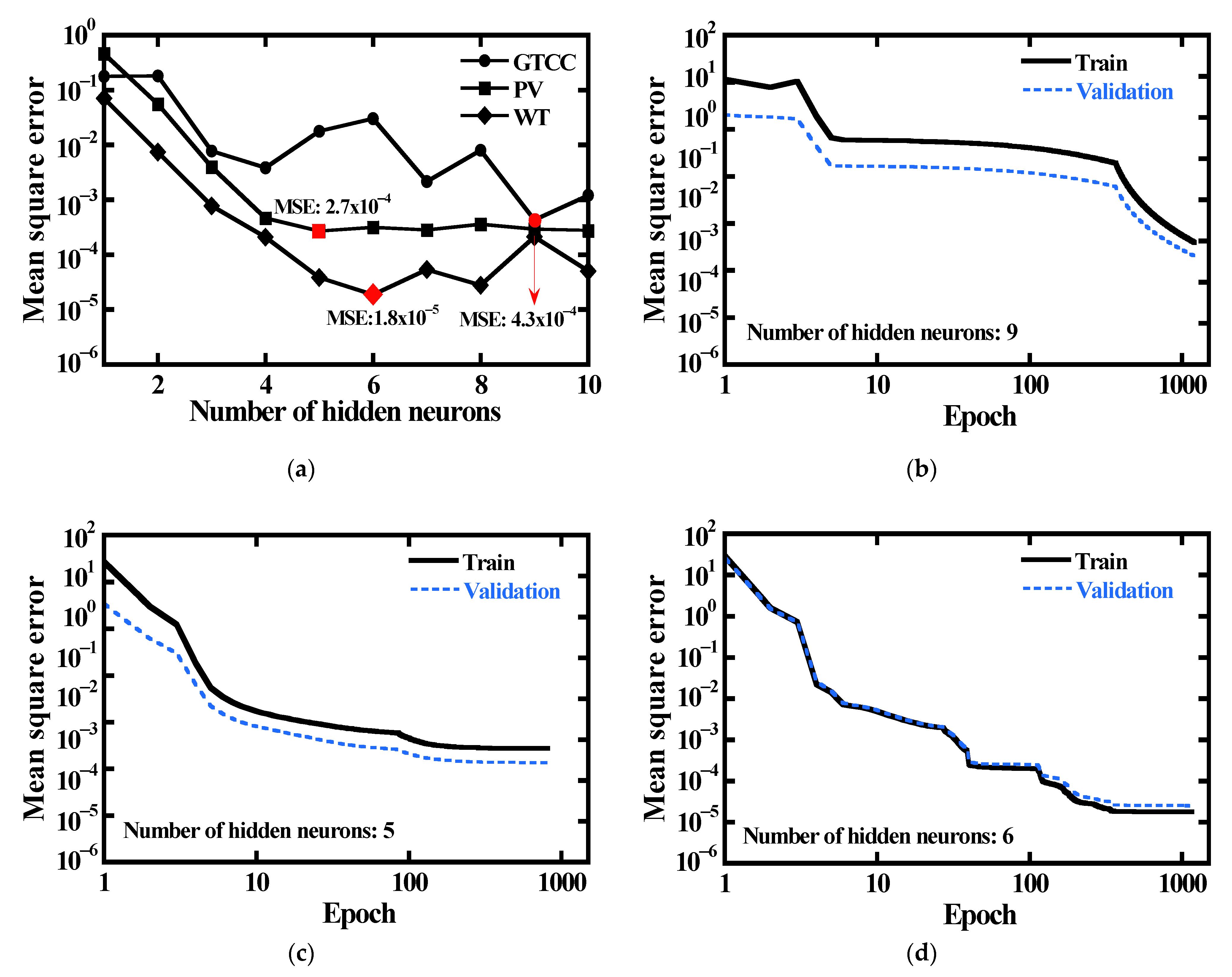
- To simplify the calculation process of the complex DG system, an ANN model was constructed. The current ANN model based on the physics-based model, unlike the conventional ANN model based on measured data, did not require a test dataset for overfitting. Therefore, a large proportion of the dataset was used for training the ANN model, so the ANN model mimicked the physics-based model very well: The MSE had a maximum of 2.7 × 10⁻⁴ and a minimum of 1.8 × 10⁻⁵. As a result, the ANN model showed an improvement of at least 5200 times and at most 22,300 times for calculation time and reduced the memory required for calculation by up to 62.3%. Therefore, the ANN model is suitable for use in the optimization calculation of the DG system.
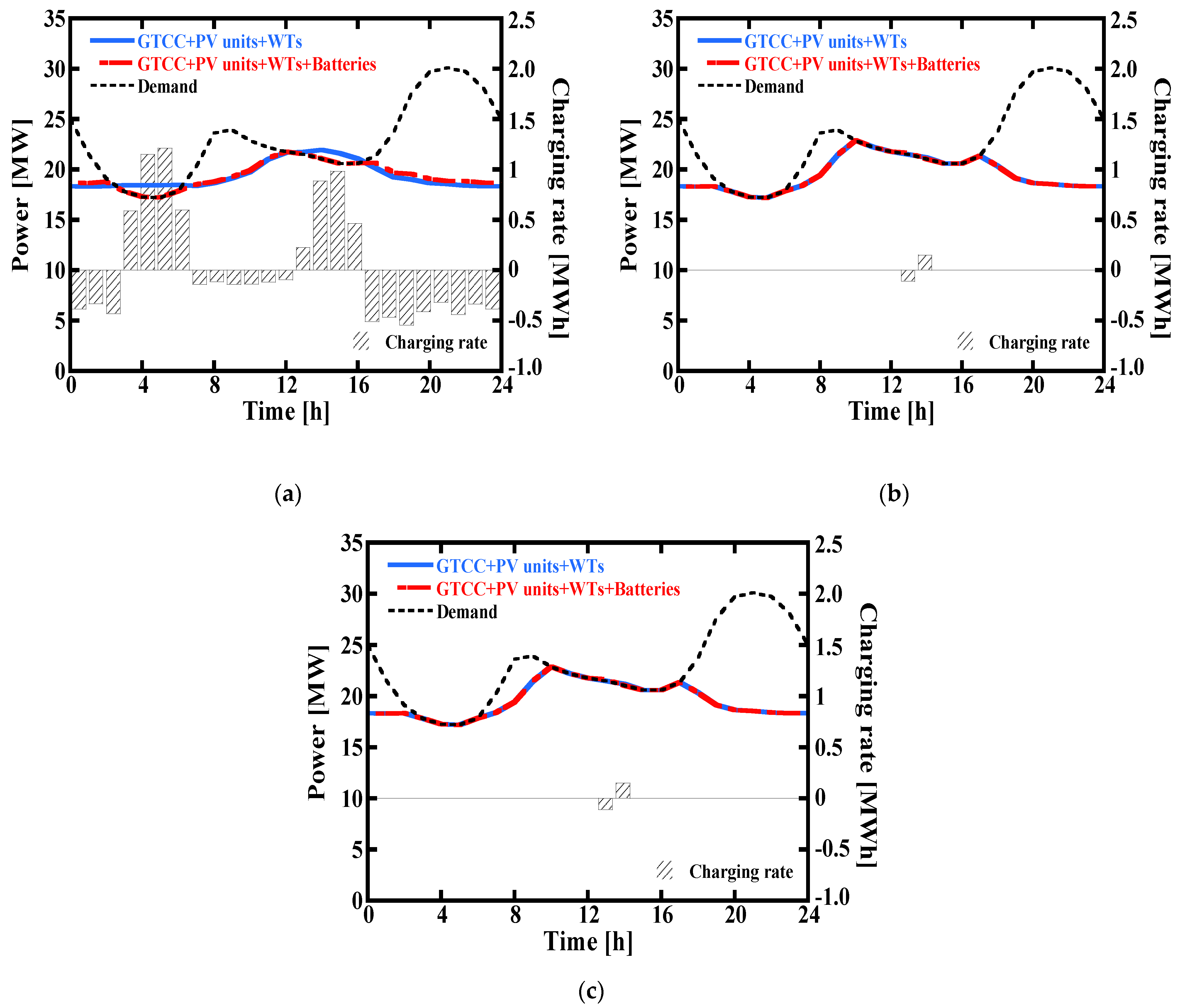
- The sizing and operation strategy of the DG system was optimized using the GA. In addition, to determine only one global optimum solution among many local solutions from GA, a weighted objective function considering eco-friendliness and cost-effectiveness was used. The optimization results were summarized for three cases according to the operation mode of the GT. In case 1, only the batteries acted as flexible resources. Hence, it had the smallest sharing rate of RE and the largest battery capacity, but had the longest life of the battery. In case 2, not only the batteries but also the GT were used as flexible resources, so the capacity of the batteries was the smallest. In case 3, the capacity of the GT is lower compared to cases 1 and 2, and it had to operate at full load. It was found to be more economical to purchase the electricity from a grid than to install the large capacity batteries, so case 3 had the smaller battery capacity than case 1. However, in case 3, the installed capacity of RE was larger, which makes the battery capacity larger than that of case 2. In cases 2 and 3, the life of the battery was shorter due to rapid charging and discharging.
- Excessive power generation compared to demand leads to an increase in required battery capacity, resulting in an increase in LCOE. In case 2, where the GT operated flexibly, the LCOE was 14.4% lower than case 1 and 42.3% lower than case 3. In other words, minimizing the role of the battery through flexible operation of a conventional generator like the GTCC is the best choice for feasible and economic performance in isolated regional DG.
Author Contributions
Funding
Institutional Review Board Statement
Informed Consent Statement
Conflicts of Interest
Nomenclature
| A | Area (m2) |
| ANN | Artificial neural network |
| a | Ideality factor (-) |
| BC | Bottoming cycle |
| C | Capacity (Ah) |
| Cheat | Heat capacity (kJ/K) |
| Cp | Power coefficient (-) |
| Cr | Heat capacity ratio (-) |
| CF | Capacity factor (-) |
| Cap | Capital cost ($) |
| Cycle | Cycles of battery (-) |
| cf | Correction factor (-) |
| DG | Distributed generation |
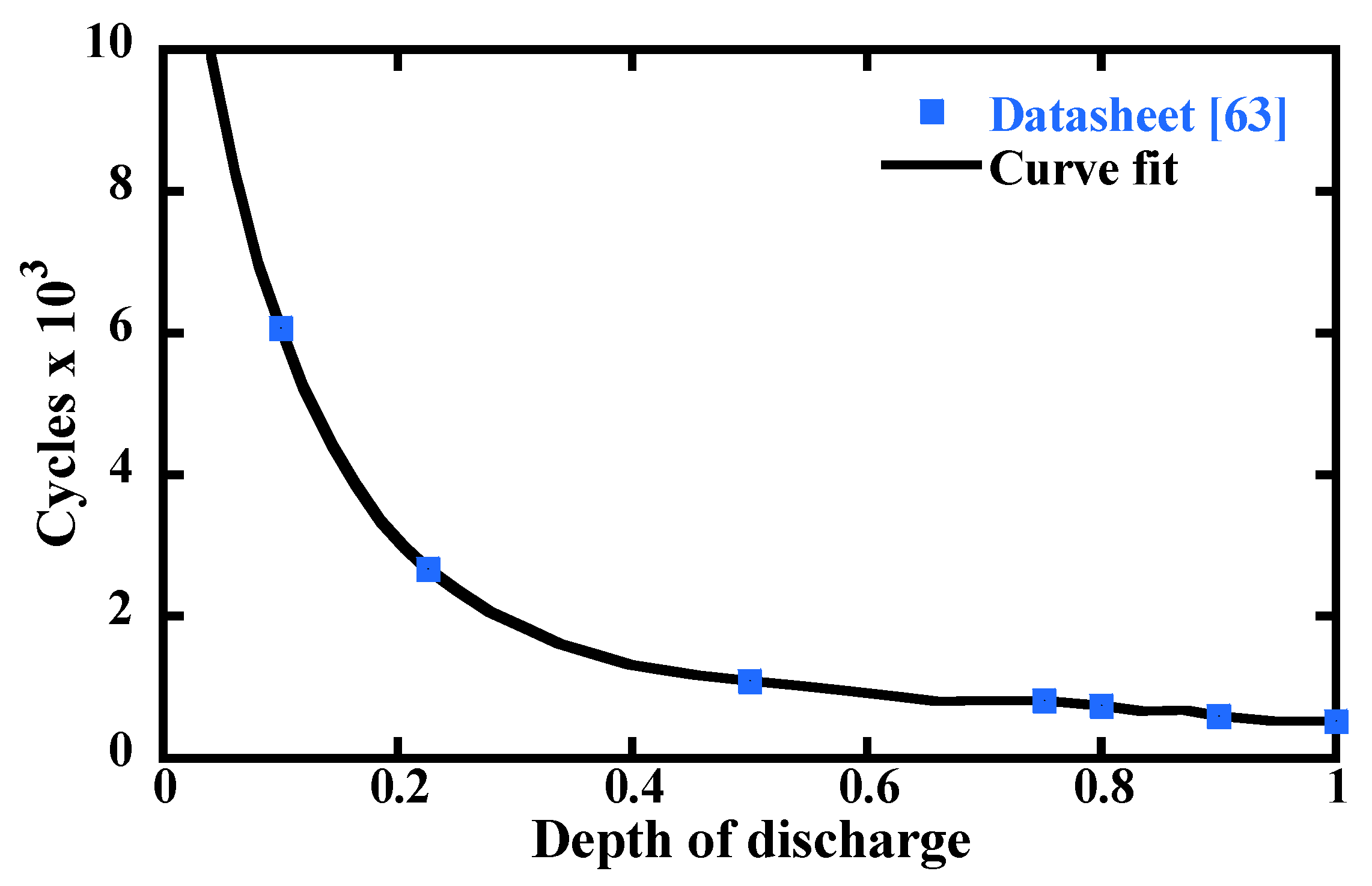
| DoD | Depth of discharge (-) |
| d | Degradation rate (-) |
| E | Electricity generation (MW) |
| ECON | Economizer |
| ESS | Energy storage system |
| EVAP | Evaporator |
| Eg | Band gap energy (eV) |
| FFN | Feed forward neural network |
| FC | Fuel cost ($) |
| G | Solar Irradiation (W/m2) |
| GA | Genetic algorithms |
| GT | Gas turbine |
| GTCC | Gas turbine combined cycle |
| I | Current (A) |
| i | Discount rate (-) |
| H | Height (m) |
| h | Specific enthalpy (kJ/kg) |
| K | short-circuit current temperature coefficient (A/K) |
| k | Boltzman constant (1.38 × 10⁻²³ J/K) |
| L | Power demand (MW) |
| LCOE | Levelized cost of electricity ($/kWh) |
| LHV | Lower heating value (kJ/kg) |
| M | Semi-dimensionless mass flow rate (ms K0.5) |
| MPP | Maximum power point |
| MPPT | Maximum power point tracking |
| MSE | Mean squared error |
| Mass flow rate (kg/s) | |
| N | Speed (rpm) |
| NG | Natural gas |
| NTU | Number of transfer unit |
| n | Number |
| OM | O&M cost ($) |
| Obj | Objective function |
| PR | Pressure ratio (-) |
| PV | Photovoltaics |
| Purel | Electricity purchase price ($) |
| P&O | Perturb and observe |
| p | Pressure (kPa) |
| Q | Charged/discharged energy (MWh) |
| q | Electron charge (1.6 × 10⁻¹⁹ C) |
| R | Resistance (ohm) |
| RE | Renewable energy |
| REC | Renewable energy certificate |
| RPS | Renewable portfolio standard |
| r | Blade radius (m) |
| S | Stored energy (MWh) |
| SMP | System marginal price |
| SPHT | Superheater |
| Salesel | Electricity sale price ($) |
| SoC | State of charge (-) |
| T | Temperature (°C) |
| t | Time (h) |
| U | Overall heat transfer coefficient (W/m2 K) |
| V | Voltage (V) |
| VIGV | Variable inlet guide vane |
| v | Wind speed (m/s) |
| Power (MW) | |
| WT | Wind turbine |
| w | Weights (-) |
| X | Electricity transaction volume (MWh) |
| Greek | |
| α | Exponent (-) |
| β | Blade pitch angle (o) |
| ε | Effectiveness (-) |
| η | Efficiency (-) |
| λ | Tip-power ratio (-) |
| λi | Constants |
| ρ | Density (m3/s) |
| Ω | Semi-dimensionless speed (rpm/K0.5) |
| ω | Rotor speed (rad/s) |
| Subscripts | |
| air | Air |
| Bat | Battery |
| c | Cold |
| ch | Charge |
| co | Corrected map |
| comp | Compressor |
| conv | Conversion |
| d | Design |
| dem | Demand |
| dis | Discharge |
| f | Fuel |
| GT | Gas turbine |
| g | Generator |
| gear | Gear box |
| h | Hot |
| in | Inlet |
| inv | Inverter |
| max | Maximum |
| me | Mechanical |
| min | Minimum |
| o | Saturation |
| opt | Optimal |
| or | Original map |
| out | Outlet |
| p | Shunt |
| ph | Light generation |
| r | Rate |
| ref | Reference |
| rem | Remain |
| rotor | Rotor |
| S | Shaft |
| ST | Steam turbine |
| STC | Standard test condition |
| s | Isentropic |
| sc | Short-circuit |
| se | Series |
| T | Thermal |
| t | Turbine |
| tot | Total |
| VIGV | Variable inlet guide vane |
| 0 | Near-surface |
| 10 | Rated charge time of battery is 10 h |
Appendix A

| Iteration | Design Variables | Objective Functions | Weighted Objective Function | |||||||||||
|---|---|---|---|---|---|---|---|---|---|---|---|---|---|---|
| Number of PV | Number of WT | Charging Rate of Battery [MWh] | LCOE [$/kWh] | Load Sharing Rate | Self-Consumption Rate | |||||||||
| 1 h | 2 h | 3 h | 4 h | … | 22 h | 23 h | 24 h | |||||||
| 1 | 207,946 | 9 | −14.58 | 3.63 | 6.89 | 8.07 | −17.40 | −17.91 | −15.57 | 676.06 | 0.28 | 0.94 | 0.63 | |
| 2 | 569,001 | 8 | −19.33 | 2.18 | 4.58 | 5.46 | −15.13 | −15.02 | −18.76 | 881.06 | 0.32 | 0.91 | 0.54 | |
| 3 | 649,810 | 5 | −10.14 | 0.66 | 3.54 | 4.68 | −9.41 | −8.65 | −8.51 | 596.26 | 0.26 | 0.93 | 0.61 | |
| 4 | 715,253 | 1 | −9.77 | −11.65 | 0.67 | 2.57 | −8.44 | −8.91 | −9.66 | 494.31 | 0.17 | 0.97 | 0.64 | |
| 5 | 709,664 | 9 | −14.63 | 2.18 | 4.13 | 4.84 | −11.69 | −11.90 | −11.53 | 876.09 | 0.38 | 0.87 | 0.49 | |
| 6 | 303 | 1 | −0.65 | −1.41 | 16.04 | 61.08 | −0.69 | −0.43 | −0.51 | 220.03 | 0.03 | 1.00 | 0.66 | |
| 7 | 687,130 | 1 | −9.29 | −12.29 | 0.72 | 2.73 | −10.89 | −9.55 | −10.93 | 476.96 | 0.16 | 0.97 | 0.64 | |
| 8 | 749,938 | 9 | −16.87 | 2.11 | 4.00 | 4.68 | −10.20 | −16.48 | −14.78 | 798.22 | 0.39 | 0.86 | 0.50 | |
| 9 | 659,032 | 9 | −19.47 | 2.15 | 4.31 | 5.05 | −13.87 | −20.55 | −18.91 | 913.85 | 0.37 | 0.88 | 0.50 | |
| 10 | 207,946 | 9 | −19.63 | 1.97 | 4.28 | 5.11 | −14.35 | −15.56 | −21.58 | 906.11 | 0.34 | 0.90 | 0.52 | |
| 11 | 427,860 | 1 | −9.07 | −9.13 | 1.54 | 5.85 | −7.79 | −7.88 | −7.77 | 318.68 | 0.11 | 0.98 | 0.68 | |
| 12 | 279,406 | 1 | −6.72 | −7.78 | 3.70 | 14.11 | −7.83 | −5.44 | −6.34 | 236.50 | 0.08 | 0.99 | 0.70 | |
| 13 | 718,296 | 9 | −17.39 | 2.11 | 4.10 | 4.80 | −15.34 | −15.06 | −14.22 | 1380.90 | 0.38 | 0.88 | 0.37 | |
| 14 | 658,993 | 9 | −19.41 | 2.15 | 4.31 | 5.05 | −13.97 | −20.45 | −18.89 | 917.29 | 0.37 | 0.88 | 0.50 | |
| 15 | 602,976 | 8 | −17.75 | 2.09 | 4.42 | 5.28 | −14.35 | −14.73 | −18.63 | 995.00 | 0.33 | 0.91 | 0.50 | |
| 16 | 716,119 | 9 | −17.46 | 2.11 | 4.11 | 4.81 | −15.33 | −14.96 | −14.51 | 1352.51 | 0.38 | 0.88 | 0.38 | |
| … | … | |||||||||||||
| 345 | 706,953 | 8 | −13.76 | 1.91 | 4.01 | 4.79 | −11.69 | −11.72 | −11.70 | 841.60 | 0.35 | 0.89 | 0.52 | |
| 346 | 751,660 | 9 | −16.24 | 2.11 | 3.99 | 4.68 | −11.55 | −16.64 | −14.59 | 804.39 | 0.39 | 0.86 | 0.50 | |
| 347 | 614,281 | 8 | −17.94 | 2.05 | 4.37 | 5.22 | −14.44 | −14.86 | −17.99 | 937.97 | 0.33 | 0.91 | 0.52 | |
| 348 | 710,349 | 4 | −10.25 | −10.73 | 2.90 | 4.10 | −9.66 | −8.06 | −8.30 | 593.94 | 0.24 | 0.94 | 0.61 | |
| 349 | 751,450 | 1 | −8.62 | −11.83 | 0.63 | 2.39 | −12.12 | −9.67 | −12.56 | 515.67 | 0.17 | 0.96 | 0.63 | |
| 350 | 359,758 | 1 | −7.78 | −7.23 | 2.10 | 8.02 | −8.16 | −7.33 | −6.91 | 279.42 | 0.10 | 0.99 | 0.69 | |
References
- Transforming Our World: The 2030 Agenda for Sustainable Development; United Nations General Assembly: New York, NY, USA, 2015.
- World Energy Outlook 2020; International Energy Agency: Paris, France, 2020.
- Dondi, P.; Bayoumi, D.; Haederli, C.; Julian, D.; Suter, M. Network integration of distributed power generation. J. Power Sources 2002, 106, 1–9. [Google Scholar] [CrossRef]
- Pepermans, G.; Driesen, J.; Haeseldonckx, D.; Belmans, R.; D’haeseleer, W. Distributed generation: Definition, benefits and issues. Energy Policy 2005, 33, 787–798. [Google Scholar] [CrossRef]
- Brandoni, C.; Renzi, M. Optimal sizing of hybrid solar micro-CHP systems for the household sector. Appl. Therm. Eng. 2015, 75, 896–907. [Google Scholar] [CrossRef]
- Ren, H.; Zhou, W.; Nakagami, K.; Gao, W.; Wu, Q. Multi-objective optimization for the operation of distributed energy systems considering economic and environmental aspects. Appl. Energy 2010, 87, 3642–3651. [Google Scholar] [CrossRef]
- Bischi, A.; Taccari, L.; Martelli, E.; Amaldi, E.; Manzolini, G.; Silva, P.; Campanari, S.; Macchi, E. A detailed MILP optimization model for combined cooling, heat and power system operation planning. Energy 2014, 74, 12–26. [Google Scholar] [CrossRef]
- Li, B.; Roche, R.; Paire, D.; Miraoui, A. Optimal sizing of distributed generation in gas/electricity/heat supply networks. Energy 2018, 151, 675–688. [Google Scholar] [CrossRef] [Green Version]
- Tutkun, N.; Celebi, N. An improved approach to minimise energy cost in a small wind-photovoltaic hybrid system. In Proceedings of the 2016 International Renewable and Sustainable Energy Conference (IRSEC), Marrakech, Morocco, 14–17 November 2016; pp. 858–862. [Google Scholar] [CrossRef]
- Moradi, M.H.; Eskandari, M. A hybrid method for simultaneous optimization of DG capacity and operational strategy in microgrids considering uncertainty in electricity price forecasting. Renew. Energy 2014, 68, 697–714. [Google Scholar] [CrossRef]
- Nayanatara, C.; Baskaran, J.; Kothari, D.P. Hybrid optimization implemented for distributed generation parameters in a power system network. Int. J. Electr. Power Energy Syst. 2016, 78, 690–699. [Google Scholar] [CrossRef]
- Morvaj, B.; Evins, R.; Carmeliet, J. Optimising urban energy systems: Simultaneous system sizing, operation and district heating network layout. Energy 2016, 116, 619–636. [Google Scholar] [CrossRef]
- Pesaran, H.A.M.; Nazari-Heris, M.; Mohammadi-Ivatloo, B.; Seyedi, H. A hybrid genetic particle swarm optimization for distributed generation allocation in power distribution networks. Energy 2020, 209, 118218. [Google Scholar] [CrossRef]
- Cedillos Alvarado, D.; Acha, S.; Shah, N.; Markides, C.N. A Technology Selection and Operation (TSO) optimisation model for distributed energy systems: Mathematical formulation and case study. Appl. Energy 2016, 180, 491–503. [Google Scholar] [CrossRef]
- Falke, T.; Krengel, S.; Meinerzhagen, A.K.; Schnettler, A. Multi-objective optimization and simulation model for the design of distributed energy systems. Appl. Energy 2016, 184, 1508–1516. [Google Scholar] [CrossRef]
- Vale, A.; Faria, P.; Morais, H.; Khodr, H.M.; Silva, M.; Kadar, P. Scheduling distributed energy resources in an isolated grid—An artificial neural network approach. IEEE PES Gen. Meet. PES 2010, 2010, 6–12. [Google Scholar] [CrossRef]
- Golestani, S.; Tadayon, M. Distributed generation dispatch optimization by artificial neural network trained by particle swarm optimization algorithm. In Proceedings of the 2011 8th International Conference on the European Energy Market (EEM), Zagreb, Croatia, 25–27 May 2011; pp. 543–548. [Google Scholar] [CrossRef]
- Kampouropoulos, K.; Andrade, F.; Sala, E.; Espinosa, A.G.; Romeral, L. Multiobjective optimization of multi-carrier energy system using a combination of ANFIS and genetic algorithms. IEEE Trans. Smart Grid 2018, 9, 2276–2283. [Google Scholar] [CrossRef] [Green Version]
- Mayer, M.J.; Szilágyi, A.; Gróf, G. Environmental and economic multi-objective optimization of a household level hybrid renewable energy system by genetic algorithm. Appl. Energy 2020, 269, 115058. [Google Scholar] [CrossRef]
- Merei, G.; Berger, C.; Sauer, D.U. Optimization of an off-grid hybrid PV-Wind-Diesel system with different battery technologies using genetic algorithm. Sol. Energy 2013, 97, 460–473. [Google Scholar] [CrossRef]
- Ogunjuyigbe, A.S.O.; Ayodele, T.R.; Akinola, O.A. Optimal allocation and sizing of PV/Wind/Split-diesel/Battery hybrid energy system for minimizing life cycle cost, carbon emission and dump energy of remote residential building. Appl. Energy 2016, 171, 153–171. [Google Scholar] [CrossRef]
- Hou, J.; Wang, J.; Zhou, Y.; Lu, X. Distributed energy systems: Multi-objective optimization and evaluation under different operational strategies. J. Clean. Prod. 2021, 280, 124050. [Google Scholar] [CrossRef]
- Mayer, M.J.; Gróf, G. Techno-economic optimization of grid-connected, ground-mounted photovoltaic power plants by genetic algorithm based on a comprehensive mathematical model. Sol. Energy 2020, 202, 210–226. [Google Scholar] [CrossRef]
- Dreiseitl, S.; Ohno-Machado, L. Logistic regression and artificial neural network classification models: A methodology review. J. Biomed. Inform. 2002, 35, 352–359. [Google Scholar] [CrossRef] [Green Version]
- Kachitvichyanukul, V. Comparison of Three Evolutionary Algorithms: GA, PSO, and DE. Ind. Eng. Manag. Syst. 2012, 11, 215–223. [Google Scholar] [CrossRef] [Green Version]
- Gen, M.; Cheng, R.; Lin, L. Network Models and Optimization: Multiobjective Genetic Algorithms Approach; Springer: New York, NY, USA, 2008. [Google Scholar]
- Ackermann, T.; Andersson, G.; Söder, L. Distributed generation: A definition. Electr. Power Syst. Res. 2001, 57, 195–204. [Google Scholar] [CrossRef]
- Sheaffer, P. Interconnection of Distributed Generation to Utility Systems: Recommendations for Technical Requirements, Procedures and Agreements, and Emerging Issues; RAP: Montpelier, VT, USA, 2011. [Google Scholar]
- Weather Data Open Portal. Available online: https://data.kma.go.kr/cmmn/main.do (accessed on 10 October 2021).
- Power Consumption Coefficient. Available online: https://kosis.kr/statHtml/statHtml.do?orgId=310&tblId=DT_3664N_2008&conn_path=I3 (accessed on 10 October 2021).
- Power Data Open Portal System. Available online: https://bigdata.kepco.co.kr/cmsmain.do?scode=S01&pcode=main&redirect=Y (accessed on 10 October 2021).
- MathWorks Inc. MATLAB R2019b; MathWorks Inc.: Natick, MA, USA, 2019; Available online: https://mathworks.com/products/matlab.html (accessed on 10 October 2021).
- McBride, B.J.; Zehe, M.J.; Gordon, S. NASA Glenn Coefficients for Calculating Thermodynamic Properties of Individual Species; NASA: Cleveland, OH, USA, 2002. [Google Scholar]
- Bell, I.H.; Wronski, J.; Quoilin, S.; Lemort, V. Pure and pseudo-pure fluid thermophysical property evaluation and the open-source thermophysical property library coolprop. Ind. Eng. Chem. Res. 2014, 53, 2498–2508. [Google Scholar] [CrossRef] [PubMed] [Green Version]
- Titan 130 Gas Turbine Generator Set (Technical Brochure); Solar Turbines: San Diego, CA, USA, 2013.
- Taurus 60 Gas Turbine Generator Set (Technical Brochure); Solar Turbines: San Diego, CA, USA, 2009.
- Saadatmad, M.; Rocha, G.; Armstrong, B. The Titan 130 Gas Turbine Performance Uprate and Operating Experience. In Proceedings of the The 16th symposium on industrial application of gas turbines (IAGT), Banff, AB, Canada, 12–14 October 2005. [Google Scholar]
- Traverso, A.; Massardo, A.F.; Lagorio, G. Widget-temp: A novel web-based approach for thermoeconomic analysis and optimization of conventional and innovative cycles. In Proceedings of the ASME Turbo Expo, Vienna, Austria, 14–17 June 2004. ASME Paper GT2004-54115. [Google Scholar]
- Do, A.-T.V. Performance and Controls of Gas Turbine-Driven Combined Cooling Heating and Power Systems for Economic Dispatch; University of California: Irvine, CA, USA, 2013. [Google Scholar]
- Kim, M.J.; Kim, T.S.; Flores, R.J.; Brouwer, J. Neural-network-based optimization for economic dispatch of combined heat and power systems. Appl. Energy 2020, 265, 114785. [Google Scholar] [CrossRef]
- Kim, M.J.; Kim, J.H.; Kim, T.S. The effects of internal leakage on the performance of a micro gas turbine. Appl. Energy 2018, 212, 175–184. [Google Scholar] [CrossRef]
- Kim, M.J.; Kim, J.H.; Kim, T.S. Program development and simulation of dynamic operation of micro gas turbines. Appl. Therm. Eng. 2016, 108, 122–130. [Google Scholar] [CrossRef]
- Gay, R.R.; Palmer, C.A.; Erbes, M.R. Power Plant Performance Monitoring; Techniz Books International: New Delhi, India, 2006; pp. 110–116. ISBN 0-9755876-0-9. [Google Scholar]
- Kang, D.W.; Kim, T.S. Model-based performance diagnostics of heavy-duty gas turbines using compressor map adaptation. Appl. Energy 2018, 212, 1345–1359. [Google Scholar] [CrossRef]
- Moon, S.W.; Kwon, H.M.; Kim, T.S.; Kang, D.W.; Sohn, J.L. A novel coolant cooling method for enhancing the performance of the gas turbine combined cycle. Energy 2018, 160, 625–634. [Google Scholar] [CrossRef]
- Lee, J.H.; Kim, T.S. Novel performance diagnostic logic for industrial gas turbines in consideration of over-firing. J. Mech. Sci. Technol. 2018, 32, 5947–5959. [Google Scholar] [CrossRef]
- Kurzke, J. GarTurb12 2012. Available online: https://www.yumpu.com/en/document/read/8602458/gasturb-12-the-gasturb-program (accessed on 10 October 2021).
- Kim, J.H.; Kim, T.S.; Moon, S.J. Development of a program for transient behavior simulation of heavy-duty gas turbines. J. Mech. Sci. Technol. 2016, 30, 5817–5828. [Google Scholar] [CrossRef]
- Zhang, G.; Zheng, J.; Yang, Y.; Liu, W. Thermodynamic performance simulation and concise formulas for triple-pressure reheat HRSG of gas-steam combined cycle under off-design condition. Energy Convers. Manag. 2016, 122, 372–385. [Google Scholar] [CrossRef]
- Kehlhofer, R.; Hannemann, F.; Stirnimann, F.; Rukes, B. Combined-Cycle Gas & Steam Turbine Power Plants, 3rd ed.; Pennwell Books: Tulsa, OK, USA, 2009. [Google Scholar]
- Meenakshi, S.; Rajambal, K.; Chellamuthu, C.; Elangovan, S. Intelligent controller for a stand-alone hybrid generation system. In Proceedings of the 2006 IEEE Power India Conference, New Delhi, India, 10–12 April 2006. [Google Scholar] [CrossRef]
- Villalva, M.G.; Gazoli, J.R.; Filho, E.R. Comprehensive approach to modeling and simulation of photovoltaic arrays. IEEE Trans. Power Electron. 2009, 24, 1198–1208. [Google Scholar] [CrossRef]
- De Soto, W.; Klein, S.A.; Beckman, W.A. Improvement and validation of a model for photovoltaic array performance. Sol. Energy 2006, 80, 78–88. [Google Scholar] [CrossRef]
- Siemens Solar Industries. Installation Guide for the Siemens Solar Industries; EBSCO Publishing: Birmingham, AL, USA, 1990. [Google Scholar]
- Wu, J.; Wang, J.; Chi, D. Wind energy potential assessment for the site of Inner Mongolia in China. Renew. Sustain. Energy Rev. 2013, 21, 215–228. [Google Scholar] [CrossRef]
- Doosan Heavy Industries & Construction Wind Power Brochure; Doosan Heavy Industries & Construction: Changwon, Korea, 2020.
- Parker, C.D. Lead-acid battery energy-storage systems for electricity supply networks. J. Power Sources 2001, 100, 18–28. [Google Scholar] [CrossRef]
- Teng, J.H.; Luan, S.W.; Lee, D.J.; Huang, Y.Q. Optimal charging/discharging scheduling of battery storage systems for distribution systems interconnected with sizeable PV generation systems. IEEE Trans. Power Syst. 2013, 28, 1425–1433. [Google Scholar] [CrossRef]
- Haoming, Z.; Soon, P.L.; Yinghai, W. Lead-acid Battery Intelligent Management System Based on TMS320F2812. Sens. Transducers 2014, 179, 108–113. [Google Scholar]
- Kim, D.; Cha, H. Analysis on Lead-Acid Battery Bank for Nuclear Power Plants in Korea. In Proceedings of the The 7th International Power Electronics and Motion Control Conference, Harbin, China, 2–5 June 2012; pp. 2118–2122. [Google Scholar]
- Bortolini, M.; Gamberi, M.; Graziani, A. Technical and economic design of photovoltaic and battery energy storage system. Energy Convers. Manag. 2014, 86, 81–92. [Google Scholar] [CrossRef]
- Copetti, J.B.; Chenlo, F. Lead/acid batteries for photovoltaic applications. Test results and modeling. J. Power Sources 1994, 47, 109–118. [Google Scholar] [CrossRef]
- Trojan Battery Company. Deep Cycle Gel Battery Datasheet; 2008; Available online: http://www.renewpowers.com/datasheets/TROJAN/GEL_Trojan_ProductLineSheet.pdf (accessed on 10 October 2021).
- Rocha, G.; Kurz, R. Field and application experience of the Titan 130 industrial gas turbine. In Proceedings of the ASME Turbo Expo, New Orleans, LA, USA, 4–7 June 2001. ASME Paper 2001-GT-0224. [Google Scholar]
- Jun, H.; Changhong, D.; Wentao, H. Optimal sizing of distributed generation in micro-grid considering Energy Price Equilibrium point analysis model. In Proceedings of the 2013 IEEE 8th Conference on Industrial Electronics and Applications (ICIEA), Melbourne, VIC, Australia, 19–21 June 2013. [Google Scholar] [CrossRef]
- Thopil, M.S.; Bansal, R.C.; Zhang, L.; Sharma, G. A review of grid connected distributed generation using renewable energy sources in South Africa. Energy Strateg. Rev. 2018, 21, 88–97. [Google Scholar] [CrossRef]
- Gas Turbine World 2014-15 Handbook; Pequot Publication: Guilford, CT, USA, 2015.
- IRENA International Renewable Energy Agency Renewable Power Generation Costs in 2018; 2019; ISBN 978-92-9260-040-2. Available online: https://www.irena.org/-/media/Files/IRENA/Agency/Publication/2018/Jan/IRENA_2017_Power_Costs_2018.pdf (accessed on 10 October 2021).
- Mundada, A.S.; Shah, K.K.; Pearce, J.M. Levelized cost of electricity for solar photovoltaic, battery and cogen hybrid systems. Renew. Sustain. Energy Rev. 2016, 57, 692–703. [Google Scholar] [CrossRef] [Green Version]
- Diaf, S.; Diaf, D.; Belhamel, M.; Haddadi, M.; Louche, A. A methodology for optimal sizing of autonomous hybrid PV/wind system. Energy Policy 2007, 35, 5708–5718. [Google Scholar] [CrossRef] [Green Version]
- Ashuri, T.; Zaaijer, M.B.; Martins, J.R.R.A.; Zhang, J. Multidisciplinary design optimization of large wind turbines—Technical, economic, and design challenges. Energy Convers. Manag. 2016, 123, 56–70. [Google Scholar] [CrossRef]
- Korea Gas Corporation Natural GAS Cost. Available online: http://www.kogas.or.kr/ (accessed on 10 October 2021).
- Ministry of Economy and Finance Currency Exchange Rate Survey Statistics. Available online: https://www.moef.go.kr/ (accessed on 10 October 2021).
- Korea Electric Power Corporation Electric Charages; 2019. Available online: https://www.sec.gov/Archives/edgar/data/887225/000119312520321121/d14114d6k.htm (accessed on 10 October 2021).
- Renewable One-Stop Business Information Integration Portal. Available online: http://onerec.kmos.kr/portal/index.do (accessed on 10 October 2021).
- Luthander, R.; Widén, J.; Nilsson, D.; Palm, J. Photovoltaic self-consumption in buildings: A review. Appl. Energy 2015, 142, 80–94. [Google Scholar] [CrossRef] [Green Version]


| Parameter | 15-MW | 5.7-MW | ||
|---|---|---|---|---|
| Value | Ref. | Value | Ref. | |
| Compressor inlet mass flow rate | 49.1 kg/s | [35] | 21.5 kg/s | [36] |
| Compressor pressure ratio | 17.1 | [35] | 12.2 | [36] |
| Turbine rotor inlet temperature | 1180 °C | [37] | 1080 °C | [38] |
| Turbine exhaust gas temperature | 495 °C | [35] | 510 °C | [36] |
| Gas turbine power | 15 MW | [35] | 5.7 MW | [36] |
| Gas turbine efficiency | 0.352 | [35] | 0.315 | [36] |
| Parameter | Value | Ref. | |
|---|---|---|---|
| 15-MW GT | 5.7-MW GT | ||
| Steam turbine inlet pressure | 1687 kPa | [39] | |
| Steam turbine inlet temperature | 225.6 °C | [39] | |
| Steam turbine efficiency | 0.75 | [39] | |
| Steam turbine outlet pressure | 100 kPa | Assumed | |
| Pinch point temperature difference | 10 °C | Assumed | |
| Exhaust gas temperature | 170.3 °C | 167.8 °C | Result |
| Steam turbine power | 2.6 MW | 1.2 MW | Result |
| Parameter | Value | Ref. |
|---|---|---|
| Open circuit voltage | 21.6 V | [51] |
| Short circuit current | 3.27 A | |
| Voltage at the maximum power point | 17.4 V | |
| Current at the maximum power point | 3.05 A | |
| Short circuit current temperature coefficient | 0.0017 A/K | |
| Maximum power output | 53 W | |
| Series resistance | 0.2 ohm | Result |
| Shunt resistance | 305.3 ohm | Result |
| Parameter | Value | Ref. |
|---|---|---|
| Cut-in wind speed | 3 m/s | [56] |
| Rated wind speed | 10 m/s | |
| Cut-out wind speed | 20 m/s | |
| Rotor diameter | 134 m | |
| Blade length | 65.5 m | |
| Hub height | 90 m | |
| Rated power | 3 MW | Result |
| Blade pitch angle | 2.3° | Result |
| Parameter | Value | Ref. |
|---|---|---|
| Nominal voltage | 2 V | [60] |
| End-of-charge voltage | 2.4 V | [59] |
| End-of-discharge voltage | 1.75 V | [60] |
| Minimum SoC | 20% | [58] |
| Maximum SoC | 90% | [58] |
| Charging efficiency | 89.5% | [61] |
| Discharging efficiency | 89.5% | [61] |
| Component | Input Data | Output Data | |
|---|---|---|---|
| Parameter | Range | ||
| Common | 0–40 °C | - | |
| Gas turbine combined cycle | 7.5–16 MW (15-MW GT)/ 2.8–6 MW (5.7-MW GT) | ||
| Photovoltaic module | 0–1000 W/m2 | ||
| Wind turbine | 0–50 m/s | ||
| Parameter | Value | Ref. | |
|---|---|---|---|
| Installation cost | GTCC | $ | [67] |
| PV | Module: 400 $/kW BoS: 400 $/kW | [68,70] | |
| WT | Turbine: 980 $/kW BoS: 980 $/kW | [69,71] | |
| Battery | 300 $/kWh | [67] | |
| Inverter | 194 $/kW | [61] | |
| O&M cost | GTCC | 3 $/MWh (variable) 0.6 M$/year (fixed) | [50] |
| Inverter | 1% of the module cost | [61] | |
| PV | 1% of the turbine cost | [69] | |
| WT | 1% of the battery cost | [69] | |
| Fuel cost | 14.7 won/MJ | [72] | |
| Electricity purchase | - | ||
| Electricity sales | - | ||
| Degradation rate | GTCC | 10% | [69] |
| PV | 0.5% | [69] | |
| WT | 0.5% | [69] | |
| Discount rate | 8% | [69] | |
| Interest rate | 5% | [69] | |
| Exchange rate | 1180 won/$ | [73] | |
| Project period | 25 years | [66] | |
| Base Price | Electricity Price | |
|---|---|---|
| Off-peak time | 7220 won/kW | 61.6 won/kWh |
| Mid-peak time | 84.1 won/kWh | |
| On-peak time | 114.8 won/kWh |
| Case | Calculation Time | Required Memory | |||
|---|---|---|---|---|---|
| Physics-Based Model | Neural Network Model | Physics-Based Model | Neural Network Model | ||
| Case 1 | Simple | 28.06 s | 0.004716 s | 423.3 MB | 175.9 MB |
| Total | 2,806,000 s | 538.7 s | |||
| Case 2 | Simple | 58.07 s | 0.002860 s | 426 MB | 160.2 MB |
| Total | 5,807,000 s | 259.8 s | |||
| Case 3 | Simple | 31.74 s | 0.003612 s | 387.8 MB | 168.8 MB |
| Total | 3,174,000 s | 362.5 s | |||
| Parameter | Case 1 | Case 2 | Case 3 | |
|---|---|---|---|---|
| PV | Number | 138,117 | 613,062 | 693,810 |
| Power | 0.5 MW | 2.8 MW | 3.2 MW | |
| WT | Number | 2 | 2 | 3 |
| Power | 1.3 MW | 1.3 MW | 1.9 MW | |
| Battery | Capacity | 7.6 MWh | 0.2 MWh | 0.6 MWh |
| Charged energy | 6.1 MWh | 0.15 MWh | 0.5 MWh | |
| Discharged energy | 4.9 MWh | 0.11 MWh | 0.36 MWh | |
| Electricity sales | 0 MWh | 0.09 MWh | 0.26 MWh | |
| DoD | 57.9% | 66.6% | 66.7% | |
| Cycles | 1005.9 | 795.8 | 795.0 | |
| Objective functions | LCOE | 0.1947 $/kWh | 0.1667 $/kWh | 0.2891 $/kWh |
| Load sharing rate | 8.0% | 17.2% | 21.5% | |
| Self-consumption rate | 99.5% | 99.9% | 99.9% | |
Publisher’s Note: MDPI stays neutral with regard to jurisdictional claims in published maps and institutional affiliations. |
© 2021 by the authors. Licensee MDPI, Basel, Switzerland. This article is an open access article distributed under the terms and conditions of the Creative Commons Attribution (CC BY) license (https://creativecommons.org/licenses/by/4.0/).
Share and Cite
Kim, H.-R.; Kim, T.-S. Optimization of Sizing and Operation Strategy of Distributed Generation System Based on a Gas Turbine and Renewable Energy. Energies 2021, 14, 8448. https://doi.org/10.3390/en14248448
Kim H-R, Kim T-S. Optimization of Sizing and Operation Strategy of Distributed Generation System Based on a Gas Turbine and Renewable Energy. Energies. 2021; 14(24):8448. https://doi.org/10.3390/en14248448
Chicago/Turabian StyleKim, Hye-Rim, and Tong-Seop Kim. 2021. "Optimization of Sizing and Operation Strategy of Distributed Generation System Based on a Gas Turbine and Renewable Energy" Energies 14, no. 24: 8448. https://doi.org/10.3390/en14248448