The Feasibility of Using Zero-Emission Electric Boats to Enhance the Techno-Economic Performance of an Ocean-Energy-Supported Coastal Hotel Building

Abstract

The topics of zero-emission/energy buildings and electric mobility are increasingly being discussed as solutions to alleviate the environmental burden caused by energy consumption and CO₂ emissions in both sectors. This study investigates a zero-energy hotel building supported by a hybrid ocean renewable energy system, which interacts with several zero-emission electric boats. Nine different combinations of floating photovoltaics (FPV) and wave energy converters (WEC) are investigated to compensate for their different fluctuations and the stochasticity of energy generation. Using TRNSYS 18 to perform modeling and simulation, a comprehensive techno-economic-environmental analysis of the hybrid system was conducted. The results indicate that when the total annual generation ratios of WEC and FPV are 76% and 24%, respectively, this combination can achieve the best energy weighted matching index (WMI). The WMI reached its maximum (0.703) when 16 boats were sailing at 15 km/h for a distance of 7.5 km. However, increasing the number of boats to 16 does not help improve economic returns or reduce the annual operational equivalent CO₂ emission factor of the hybrid system. Depending on the maximum number of electric boats designed for this study, the non-dominated WMI would be limited to 0.654.

1. Introduction and Background

1.1. Background

According to the International Energy Agency (IEA), in 2018, buildings and transportation accounted for the first- and second-largest shares of global final energy use, at 36% and 28%, respectively [1]. In the Hong Kong Special Administrative Region (HKSAR), the total energy consumption of buildings and transportation accounts for about 95% of end-use energy consumption. Commercial accommodation and maritime transportation account for more than 13% and 8% of the corresponding sectors, respectively [2]. The “HK Climate Action Plan 2030+” report [3] responds to the Paris Agreement [4] by proposing an ambitious multilateral treaty with an overall 40% reduction in energy intensity by 2025, with respect to the levels in 2005. In consideration of the fact that the building and transportation sectors are the primary electricity consumers and contribute the most carbon emissions, zero-emission/energy buildings (ZEBs) and zero-emission/energy electric vehicles (ZEVs) have been proposed and studied to achieve equivalent reductions in CO₂ emissions and primary energy consumption. In addition, with strong government support, ZEBs and ZEVs have become increasingly popular in recent years, and the integration of ZEBs and ZEVs has gained attention, showing very promising potential for energy savings and energy flexibility.

1.2. Literature Review for ZEB, Electric Mobility and Ocean Renewable Energy System

In 2010, the Energy Performance of Buildings Directive (EPBD) recast (2010/31/EU) introduced the nearly zero-energy consumption target [5]. The main objective of the recast EPBD was to reduce the primary energy consumption of buildings. To achieve the goal, every new building in each EU Member State (MS) is required to become a nearly zero-energy building (NZEB). More and more papers and studies about ZEBs are emerging. Back in 2009, Wang et al. discussed the possible solutions for zero-energy building design in the UK. They applied two simulation software packages (EnergyPlus and TRNSYS 16) to obtain the best design strategy for a typical home and energy system [6]. Attia et al., for hot climate regions such as Egypt, proposed energy-oriented software tools with information support to facilitate decision making for zero-energy buildings [7]. A study by Sobhani et al. addressed the vulnerabilities of optimizing renewable energy systems in nZEBs based on present-day climate and energy price data (traditional optimization methods). They proposed a future-oriented approach to system design that can adapt to the effects of climate change and energy price changes with minimal life-cycle costs [8]. The feasibility of technologies as applied to ZEB was reviewed by Cao et al. They found that improvements in building envelope and ventilation could play an essential role in reducing space heating and cooling consumption levels, as a major need for significant climate change [9]. In [10], Arabkoohsar et al. studied a novel system’s technical and economic aspects, they evaluated and compared with other conventional solar-based building energy systems consisting of PV panels integrated with battery and heat pump interacting with the electricity grid. Sakdirat et al. proposed optional solutions and applied PV and wind systems to achieve the NZEB goal for an existing townhouse in Washington, DC [11]. Since 2013, hotels have also started to receive attention, considering the current limitations of NZEBs. Even more strategies have been designed for use in nearly zero-energy cities. Gholami et al. investigated the scalability of nearly zero-energy concepts using BIPV technology from individual buildings to entire cities [12]. The European initiative Nearly Zero-Energy Hotels—neZEH (www.nezeh.eu, accessed on 10 December 2021), aiming to accelerate the renovation of existing hotels, became NZEBs [13]. Tournaki et al. presented the results of 16 pilot hotel projects from seven European countries that are working to transform into NZEBs, assessing their current energy situation and proposing feasibility studies for appropriate energy efficiency and renewable energy measures [13]. M. Beccali et al. conducted a study of a hotel located on the Italian island of Lampedusa that considered several energy retrofit options in response to the development of renewable energy sources and building automation control technologies [14]. Cunha et al. analyzed a typical four-star hotel operation in Portugal to establish realistic energy performance values for NZEB hotels, which helped establish a benchmark for realistic neZEH [15]. In a study by Nocera et al., a case study was presented on an energy retrofit of an existing historical hotel located in southern Italy (Siracusa) to achieve NZEBs status [16].

In addition to the construction sector, the transportation sector also accounts for a large share of carbon emissions. Greenhouse gas emissions from transportation come primarily from burning fossil fuels in cars, trucks, ships, trains, and aircraft. More than 90% of transportation fuels are petroleum based, consisting primarily of gasoline and diesel fuel [17]. In the transportation sector, electric vehicles are being encouraged to replace fossil-fueled vehicles, helping to accelerate the deployment of low-emission alternative energy sources [18]. The electric vehicle market is so mature that much of the research focuses on charging technology for EVs. In addition to traditional charging at the charging station, more efficient and economic sources and modes of charging methods have been discussed. For example, Hafez et al. conducted an optimal design study of an electric vehicle charging station (EVCS) to minimize life-cycle costs. They found that it would be the most economically advantageous option when the EVCS is within the city limits and could be used as a smart energy center using a combined diesel–solar PV-battery energy storage system supply option [19]. Sun proposed the optimal design of a Fast Electric Vehicle Charging Station with Wind Power, Photovoltaic and Energy Storage system (FEVCS-WPE) [20]. Kumar and Cao’s paper reviewed recent advances in positive energy buildings and communities, and mentioned the impact of smart energy grids and new energy vehicles interacting with positive energy buildings and communities [21]. A study by Golla et al. presented a power-sharing model and scheduling method for V2G deployment between EVs and the grid. The results showed that to realize good benefits of distributed energy systems via EVs, the planned execution of the charging scheme is key to evaluating its impact on the power grid [22]. In addition to the different ways in which electric vehicles are charged, the interaction between buildings and EV has also received some attention. Buonomano studied the energy and economic performance of different V2B2 energy management solutions, including residential buildings, office buildings and electric vehicles, and showed that the V2B2 solution resulted in remarkable exploitation of off-site renewable energy production helping achieve a significant reduction in fossil fuel consumption in the grid [23]. Chen et al. also conducted a V2B model research in Shanghai, where they found that the HDPV-V2H model in their group could fully meet the sunny and cloudy day household load electricity demand without additional grid power, while the combination of PV and V2H shifted valley power was sufficient to support the rainy day household load demand [24]. Cao et al. investigated the impact of electric vehicles and mobile boundary expansion on the realization of zero-emission office buildings. This study involved both B2V and V2B functions. The study results show that the extended boundary could improve the matching ability of on-site renewable energy, leading the EV energy storage to be almost entirely covered by renewable energy (96.9%) [25].

Meanwhile, with the development of electric vehicles, electric boats have also gradually entered the mass market. As reported in a 2014 news article, YC Synergy developed fuel cells ranging in power from 1 kW to 6 kW that could be used in series or parallel to generate higher voltages for larger passenger and tour boats. YC Synergy’s electric boat solutions combine its proprietary PEM fuel cell technology with various battery and boat motor products, and even solar panels that are seamlessly integrated to meet propulsion and energy management needs [26]. Al-Falahi et al. used two optimization techniques to optimize the power of hybrid power systems in electric ferries [27]. In the study by Kim et al., they conducted the design of a DC shipboard power system for a purely electric propulsion ship based on a battery energy storage system via MATLAB [28]. Recently, Tercan et al. investigated a group study considering a solar-assisted boat in which an off-grid rooftop photovoltaic system with 9.8 kWh batteries was installed to meet the energy demand for internal services and to reduce diesel use. This solar-assisted vessel proved to be an economical solution. Their findings showed that a variety of off-grid rooftop PV systems can be applied for sustainable transport and help to reduce the operating costs of the boat [29].

In addition to the more popular wind and photovoltaic power, other renewable energy sources are also entering the market to support building demand and electric vehicle demand. In particular, the Southeast Asian region (SEA) is surrounded by the ocean, from which there is a vast potential to harness energy. Waves, tidal energy, and ocean thermal energy conversion can be harnessed to provide the region with clean and reliable alternative energy sources. Quirapas et al. examined the current activities of ocean renewable energy (ORE) and ocean region countries. Their paper examined the current status of ORE energy in Southeast Asia from various perspectives, including technological, socioeconomic, environmental, and political factors. They found that ORE technologies were suitable for local conditions in Southeast Asia, and that the development of ORE will bring socio-economic benefits such as employment opportunities, inter-industry learning, economic resilience, and investment [30]. As investigated by Quirapas et al., many Southeast Asian countries have started to exploit ocean energy. For instance, in Singapore, the Minister of Environment and Water Resources Masagos Zulkifli launched the world’s largest floating solar PV cell testbed in 2016, measuring 1 hectare and containing ten different solar PV systems [31]. Furthermore, a tidal energy demonstration project began generating electricity in 2019. The team installed Mako turbines under the Sentosa Boardwalk. The electricity generated through the project is fed into the grid to support lighting along the Sentosa Boardwalk [32]. Meanwhile, in 2018, approval granted by the Philippine Department of Energy gave Oceantera the right to begin activities related to the pre-development of a utility-scale tidal energy project on a 2600-hectare site in the San Bernardino area of the Philippines [33]. Moreover, other coastal countries and areas have also conducted many kinds of research on ORE. For example, Lavidas performed a study on the potential for unlocking wave energy in the EU, which concluded that there are regions with “hidden” opportunities to accelerate proof-of-concept and increase the viability of wave energy [34]. The feasibility of ocean renewable energy in Australia is also investigated and discussed by Hemer et al., they stated that the advantage of ocean renewable energy in the energy solution mix is that it is less variable and more predictable than alternative renewable energy solutions such as wind or solar. However, some technical challenges remain, such as developing technologies to produce the best energy at the lowest cost with minimal environmental impact [35]. In addition, ocean thermal energy and other ORE technologies have also attracted attention. Romero et al. proposed a nonlinear programming (NLP) multi-period and multi-objective model for analyzing ocean thermal energy conversion systems. They studied the variability of solar resource availability, energy demand, and environmental conditions to support a specific residential building located on Mexico’s Pacific coast [35]. Jiang et al. introduced a hybrid ocean wave-current energy converter (HWCEC) that drew energy from ocean waves and currents simultaneously with a single power takeoff [36]. Weiss et al. developed and implemented an innovative approach to identify potential wind and wave energy development areas on a global scale [37].

1.3. Scientific Gaps and Structure of the Study

Based on the literature review described above, several scientific gaps can be noticed in the international academic community: firstly, previous international research has focused more on the refurbishment of existing hotels. Some researchers have mentioned achieving the goal of nearly zero-energy buildings with renewable or semi-renewable energy systems, but few researchers have mentioned applying ocean renewable energy. Both Hong Kong and Mediterranean areas are tourism hotspots with geographical advantages, and there are limited studies on the different combinations of ocean renewable energy for hotel buildings. This study will investigate the feasibility of two ocean renewable energy systems to support the hotel building needs. These two ORE systems will bring more ideas for further study to achieve the NZEB goal in the future.

Secondly, although there are many studies on EVs nowadays, most of them focus on the charging methods/sources of EVs, while some researchers have studied the interaction between EV and buildings. For example, Chen et al. studied vehicle-to-home [24], and Cao et al. conducted studies on both B2V and V2B [25,38]. As for the electric boat, more attention has been paid to using renewable energy systems, such as PV panels, to replace traditional diesel-powered tourist boats. However, the interaction among electric boats, buildings and REe is rarely mentioned.

Thirdly, various OREs have been widely discussed in academic circles, such as floating PV, tidal in-stream, wave, and ocean thermal. The potential of OREs in the SEA region can be seen from the article by Quirapas et al. [30], which also shows that it is promising in most coastal countries and areas. Nevertheless, most studies are more concerned with the application, obstacles, and potential of ORE technology. There is little research that focuses on the application of OREs to support buildings. Moreover, few studies address technical, economic, and environmental considerations.

Based on these three scientific gaps, this paper focuses on a hybrid Wave-FPV device-supported zero-emission coastal hotel building that interacts with the zero-emission electric boats. Different energy control strategies will be applied and investigated in this study. The impact of the cruise velocity, cruise range, cruise schedule and the V2B interactions will be determined and comprehensively investigated. Furthermore, the techno-economic-environmental analysis of different situations will also be performed. In the following sections, the integrated hybrid system, simulation environment, weather, building and boat energy demand will be introduced in Section 2. Section 3 will present a description of the boat control principles and ocean renewable energy system, and the analysis criteria of energy matching ability, economic index and the environmental index will be described in Section 4. In Section 5, the simulation results, analyses, and discussion will be presented. The conclusion will be given in Section 6.

2. System Description and Assumptions

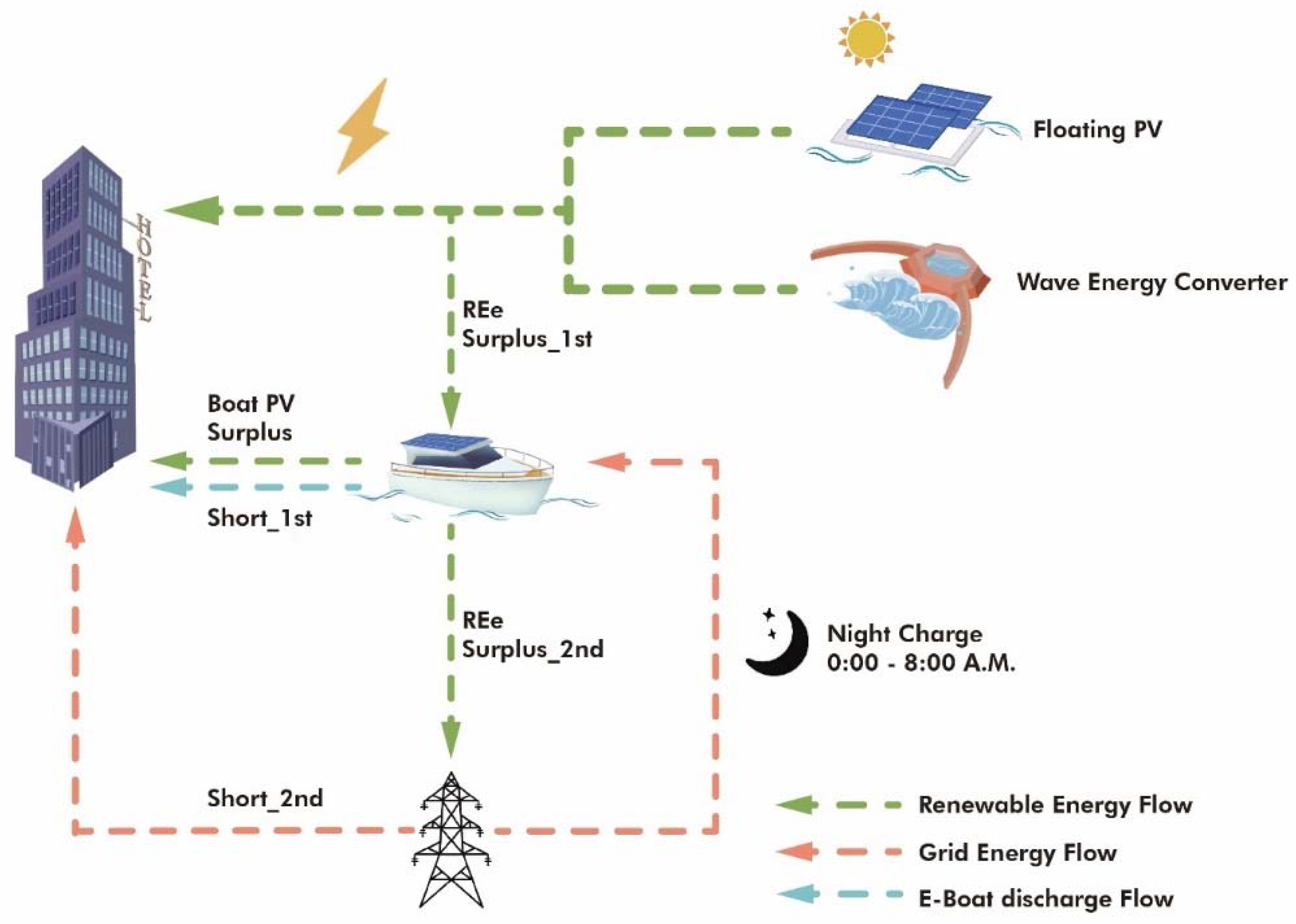
2.1. The Basic Components and Control Principal

A brief schematic of the hybrid system is depicted in Figure 1. The hybrid system includes two different ocean renewable electricity generation systems, the building’s electricity-consuming devices, and the integrated electric boat system. The renewable electricity generation systems are composed of a floating photovoltaic system (FPV) and a wave energy converter device (WEC). Detailed information about the FPV and WEC is provided in Section 3.2.

All the equipment in the studied building is powered by electricity. These electric devices include water-cooled chillers (for AHU cooling and space cooling), cooling towers, auxiliary electric heaters (for domestic hot water demand), and building devices and equipment. The integrated electric boat system is composed of a battery, which can be charged and discharged to support the building, while the boat’s PV can charge the boat’s battery during trips, and when the boat is moored in port, the boat’s PV generation can provide support to the hotel building; detailed control strategies for the electric boat are described in Section 3.1, below.

As briefly illustrated in the control logic of the hybrid system presented in Figure 1, the renewable electricity generated by the renewable generation system is sent to the hotel building to cover the electric demand. If the renewable energy (REe) is higher than the building’s electricity demand (i.e., if “REe Surplus_1st” exists, as shown in Figure 1), then the surplus electrical energy will be used to charge the batteries of the E-boat. After that, if there is still any surplus energy, the surplus REe will be exported to the electric grid (i.e., if “REe Surplus_2nd” exists, as shown in Figure 1). In addition, as mentioned above, the boat PV power will be used to support the hotel building when the E-boat is moored in the harbour (i.e., if “Boat PV Surplus” exists, as shown in Figure 1). On the contrary, when the building’s electricity demand is higher than the renewable energy (i.e., if “Short_1st” exists, as shown in Figure 1), the shortage will initially be covered by discharging the batteries of the E-boat if a boat is moored in the harbor. If there is still any energy shortage (i.e., if “Short_2nd” exists, as shown in Figure 1), the rest of the electricity shortage will be imported from the electric grid.

All simulations and components consisting of buildings, electric boats and ocean renewable energy systems are performed in TRNSYS 18 [39]. TRNSYS is a complete and scalable simulation environment for transient simulations that has been developed over more than 40 years. This software can be used to simulate new energy management concepts, from simple domestic hot water systems to the design and simulation of buildings and HVAC systems, including control strategies, occupant behavior, renewable energy systems. All individual component models, also referred to as “types”, are connected with each other to build and simulate a near-realistic environment in order to calculate the performance of a system. The time step used in the simulations performed in this study is 0.25 h, which ensures the stability and convergence of the system models.

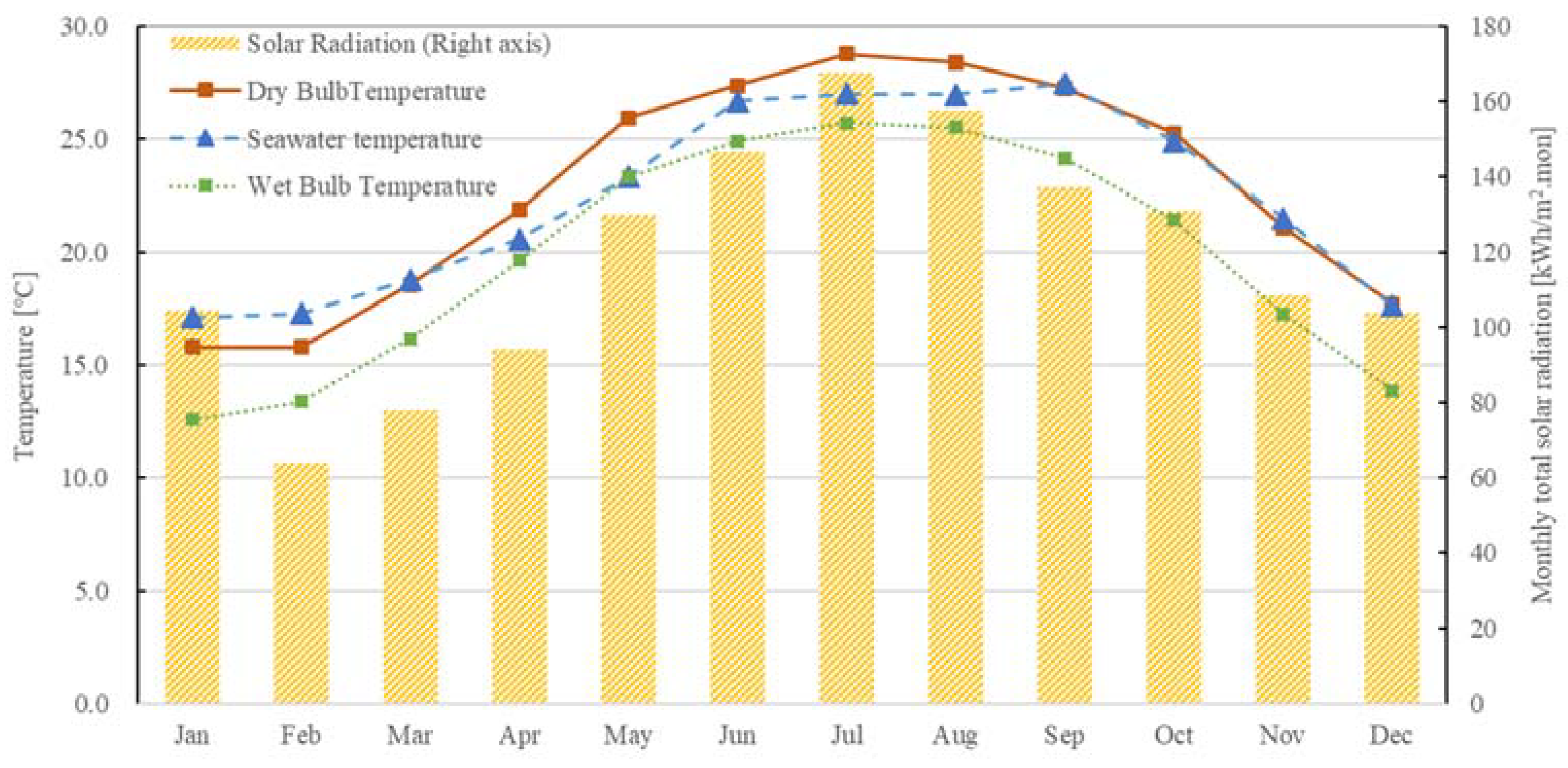
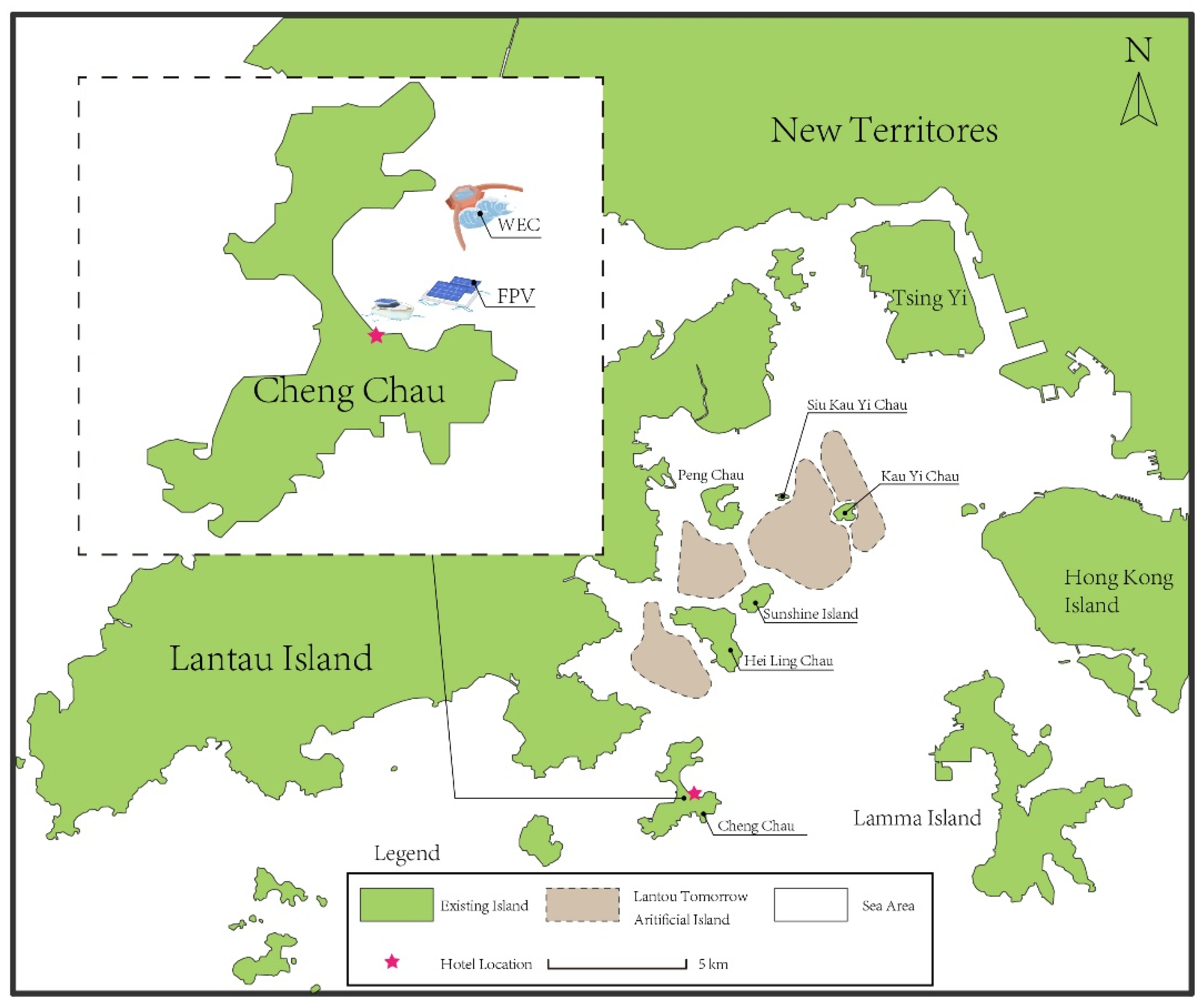
2.2. Weather and Building Service System

We studied a coastal hotel building located in Hong Kong. The city of Hong Kong has a humid subtropical climate (Köppen Cwa) [40], characteristic of southern China, despite being located south of the Tropic of Cancer (22.3° N, 114.2° E). The weather files used were obtained on the basis of Meteonorm data in Hong Kong, and included hourly weather data such as temperature, humidity ratio, solar radiation and wind velocity [41,42]. According to meteorological documents, including detailed data reporting the annual average dry bulb temperature and the total annual solar radiation on the horizontal plane, which are 22.9 °C and 1423 kWh/m².a, respectively. The calculated base temperature for annual cooling degree days and annual heating degree days is 18 °C, with 2025 cooling degree days and 247 heating degree days.

The seawater temperature data were obtained from the Hong Kong Observatory, recorded at Waglan Island in 2017. Figure 2 shows the monthly dry and wet bulb temperature, seawater temperature, and total solar radiation. Changes in both dry bulb temperature and solar radiation follow patterns in the northern hemisphere. The summer experienced high temperatures and quite intensive solar radiation. In winter, both of them correspond to a slight decrease. The year-round variation in wet bulb temperature is consistent with the variation in dry bulb temperature, but overall is about 3 °C lower than the dry bulb temperature. The monthly average seawater temperature is slightly lower (around 2 °C) than the dry bulb temperature from April to August. This is most pronounced in May, when the seawater temperature is 2.6 °C lower than the air temperature. However, during the winter months, especially in January and February, seawater temperatures are higher than dry bulb temperature (around 1.3–1.5 °C).

The historically recorded wave data were collected from West Lamma Channel monitoring stations in hourly intervals and recorded in EXCEL format, which was supported by the Civil Engineering and Development Department of Hong Kong. The historical records of waves in 2019 are adopted in this study to model wave energy conversion. It is worth noting that the historical wave records in 2019 had missing data at some time points, and the missing data were finally filled in using historical data from 2017 and 2018. The recorded data show that the annual average significant wave height is 0.34 m. The monthly significant wave height is illustrated in Figure 3. The monthly average wave height is around 0.25–0.47 m over the course of a year. February and July are the months in which the waves exhibit their minimum and maximum height during the year, with heights of 0.01 m and 0.94 m, respectively.

The studied coastal hotel building is located on Cheng Chou island, as shown in Figure 4, near Lamma Island. The proposed hotel building is a new hotel that has eight floors above ground, each with a floor area of 480 m² and a floor height of 3 m. The total floor area is 3840 m². All the building design strategies followed the Performance-Based Building Code of Hong Kong [43]. The design parameters and principles for the building envelopes, insulation and service systems are listed in Appendix A. Figure 5 illustrates the total annual energy demand and peak power demand for air handling unit (AHU) cooling, space cooling, AHU heating, space heating, domestic hot water heating, reheater heating and building electrical demand. The corresponding duration curves are also shown in Figure 4. As presented in

Table 1. The cooling, heating and electric demand of the hotel building.

	Heating				Reheater	Electric 1	Cooling
	AHU Heating 2	Space Heating	DHW Heating	Total Heating (Excluding Reheater Heating)	Reheater Heating	Electric 1	AHU Cooling	Space Cooling	Total Cooling
Total Energy (kWh/m2.a)	0.01	0.06	67.78	67.85	15.6	102.7	164.88	41.1	205.99
Peak Power (kW)	22.5	7.59	68.4	75.7	14.79	100.94	146.78	98.49	227.82

¹ Electricity demands includes lighting, equipment, and ventilation fans, but does not include cooling/heating systems or electric boat systems. ² The AHU heating demand here does not include the demand for reheaters equipped with cooling coils.

and Figure 5, the building electricity demand includes lighting, equipment, and ventilation fans, but excludes electricity for cooling and heating systems and electric boat systems. The annual total heating, cooling and electric demands are 67.85, 205.99 and 102.70 kWh/m².a, respectively.

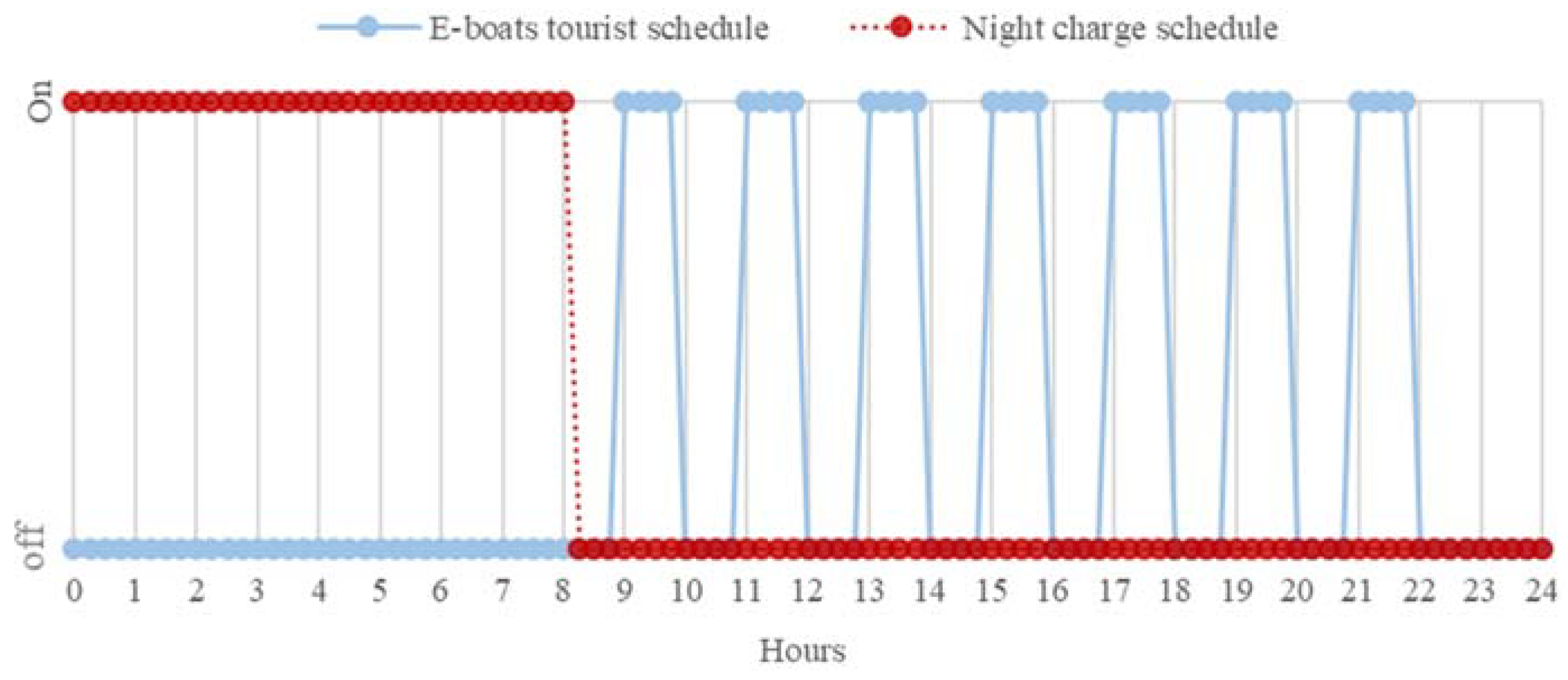
2.3. Introduction and Assumptions Regarding the Zero-Emission Boat

At the pier near the hotel, it is assumed that there is a maximum of eight electric boats available to the hotel for sightseeing purposes. The number of boats will be set as one boat in Section 5.2, Section 5.3.1, Section 5.4.1 and Section 5.4.3. More boats will be considered in Section 5.3.2 and Section 5.4.2 The maximum number of people in the hotel is 19 for each floor, which follows the building code for Hong Kong. Each boat can serve approximately 12–20 people [44]. Therefore, the design idea is that each floor is able to have one boat for excursions. As shown in Figure 6, the daily tourist schedule of the E-boats starts at 9:00 a.m. and continues until 10:00 p.m. every day, with sightseeing activities starting every 2 h. All the boats participate in the excursion activities with the same schedule. The default cruise distance of boats is assumed to be 7.5 km around the surrounding sea, and the default velocity of the boats is assumed to be constant (10 km/h) at all times during sailing, in order to facilitate the calculation of the energy consumption of the boats. The assumption of cruising velocity and distance was made with reference to local tourist boats. During the non-working hours, is the boats default to REe charging mode once they are docked at the harbour. Night charge mode is activated from 0 a.m. to 8 a.m. to guarantee the regular occurrence of the scheduled trips the following day. The detailed charging management of the E-boats is described in the following section.

The zero-emission electric boat is based on the commercial product, “Soelcat 12” [44]. It has two marina-grade lithium polymer batteries, each with an overall capacity of 60 kWh. The “Soelcat 12” is equipped with 8.6 kWp lightweight PV panels as part of the design, which boost the efficiency by 22.5%. It is worth noting that since the manufacturer has not provided specific data and information on the boat PV; therefore, in order to be able to perform the simulation on TRNSYS, another commercial product, called LG NEON, was used [45], which is a monocrystalline silicon product with a high module efficiency that can reach about 19.7%. According to simulations, the annual efficiency in the Hong Kong climate would be 18.61%. In this study, each E-boat will eventually be equipped with 25 units of PV with a total capacity of 8.5 kWp.

According to the product datasheet of this E-boat [44], when the boat travels at a velocity of 6 knots (11.11 km/h), its maximum travel time is 15 h, i.e., 168.68 km. Assuming that the battery capacity needed to drive the boat to this maximum distance is 80% of the total capacity, a final energy consumption of 0.58 kWh/km per hour can be calculated for this velocity. Correspondingly, when the velocity of the boat is 7 knots (12.96 km/h), its maximum cruise time is 10.91 h. Thus, the maximum cruise distance should be 141.44 km, and the energy consumption per hour will be 0.68 kWh/km; assuming a linear relationship between the travel velocity of the boat and its energy consumption, it can be found that when the travel velocity of the boat is 10 km/h, its energy consumption will be 0.52 kWh/km. After applying the same calculation method, the corresponding energy consumption is 0.3, 0.39 and 1.13 kWh/km at sailing velocities of 6, 7 and 15 km/h, respectively. Although the maximum energy consumption of the boat in this study is 1.13 kWh/km, each boat’s total annual energy consumption is about 0.85–1.7% of the total energy demand, considering that the distance, time, and frequency of the boat’s excursions are not high. The other velocities and corresponding energy consumptions are presented in

Table 2. E-boat velocities and corresponding energy consumptions.

Velocity (Knot)	3.2	4.0	5.4	6.0	7.0	8.0	8.1	9.0
Velocity (km/h)	6.00	7.50	10.00	11.11	12.96	14.82	15.00	16.67
Energy consumption (kWh/km)	0.30	0.39	0.52	0.58	0.68	1.08	1.13	1.58

and Figure 7, below. The control strategies and analysis of the different cruising velocities with the E-boats are described in Section 5.

3. Integrated Boat and ORE Systems

3.1. The Control Principles for Integrating the Zero-Emission Boat

As mentioned in Section 2, the studied zero-emission electric boat was designed based on the commercial product “Soelcat 12” [44], which is produced by a Dutch company called SOEL YACHTS. Soelcat 12 is supported by two batteries, and each one has a capacity of 60 kWh. In TRNSYS, the battery is modeled using TYPE 47a [46]. The upper and lower limitations of the fractional state of charge (FSOC) of the boat battery are 0.95 and 0.3, respectively. In this study, the charging and discharging modes are introduced as follows:

1.

The control strategy for the normal charging mode (building-to-boat function):

The E-boat tourist working schedule is from 9:00 a.m. to 10:00 p.m. every day, as shown in Figure 6; the cruise frequency is one trip every 2 h. The cruise time of the boat is affected by the velocity and distance, which will be discussed in Section 5.2. Whenever the unoccupied E-boat is docked in the harbour, the FSOC of the battery is below 0.95. Meanwhile, if surplus renewable energy from generation exists, the boat battery can be charged until it reaches the upper limitation of FSOC.

2.

The control strategy for night charging mode (building-to-boat function):

To ensure the planned tourist cruises take place the following day, when the FSCO of the boat is lower than 0.85, a mandatory night charging mode is activated, and the boat battery is charged from the electrical grid from 0 a.m. to 8 a.m. if there is no surplus renewable energy. The charging set point is fixed at 0.85 not only to avoid running out of battery during daytime, but also to help reduce the reliance on the electricity grid. When night charge mode is activated, the boat battery no longer discharges to support the building.

3.

The control strategy for discharging mode (boat-to-building function):

When the boat is moored with a higher FSOC than 0.8, while the generation of renewable energy is insufficient (i.e., “Short_1st” exists, as shown in Figure 1), the boat is able to discharge its battery to support the electricity demand. This means that the boat-to-building function can only be activated within an FSOC range of the battery between 0.95 and 0.8. The discharge mode should be terminated when the FSOC reaches 0.8.

3.2. The Integrated Ocean Energy System

As mentioned in Section 2.1, the integrated ocean renewable energy generation (ORE) system is composed of a floating photovoltaic system (FPV) and a wave energy converter system (WEC). Detailed information on these two systems is provided in the following sections.

3.2.1. Floating PV Panels

The FPVs are installed near the coastal area of the studied project, as shown in Figure 4. The simulation of FPVs is modeled using TRNSYS Type 567 [47]. Type 567 is a model used for modeling buildings with integrated photovoltaic systems. Considering the environment on the water is quite different from the environment on the ground, this part of the simulation environment can also be modeled using TYPE 567 by setting the back-surface temperature referrer to the seawater temperature. The seawater temperature data were obtained from the Hong Kong Observatory, recorded at Waglan Island in 2017. The reference FPV is a commercial product called FuturaSUN [48], a polycrystalline photovoltaic with 60 cells in each module. The efficiency of this applied FPV (FU 260 P) is 15.92% under standard test conditions (incidence radiation of 1000 W/m² and reference temperature of 25 °C). The dimensions of each FPV modular are 1650 mm × 990 mm × 35 mm.

There are three main reasons to apply FPV instead of rooftop PV or BIPV. First, the studied hotel is located in Hong Kong, where land use is limited. Covering all the electricity demand using a mainstream PV system is challenging, since the roof can only provide an area of 480 m². A full PV system would require more than 5000 m². Moreover, the 90-degree application of BIPV reduces the efficiency of PV. However, FPV could achieve better efficiency thanks to the lower temperature of seawater. The last point is that the application of FPV can reduce solar radiation, inhibit harmful algae growth and improve seawater quality.

3.2.2. Wave Energy Converters

The simulation and modeling of WECs are based on the commercial product called “Wave Dragon” [49]. This crab-shaped product collects the seawater arriving with the waves, then collects it through a reservoir, and finally generates electricity through the gravitational potential energy of the seawater pushing the turbine at the bottom. Each unit of WEC possesses a rated capacity of 20 kW. Similar to the modeling environment of FPV, wave energy converters can be installed around the FPV area, thus helping to provide a quiet water environment for FPV and reducing the effect of waves. The location of the WECs is illustrated in Figure 4. The simulation of wave energy conversion is driven by the formula below [50,51,52], where overtopping power is the potential power of the waves overtopping the ramp crest of the device while assuming constant efficiencies of the various components of the power take-off system:

$${\mathrm{P}}_{\mathrm{act}}={\mathrm{P}}_{\mathrm{Crest}}·{\mathsf{\eta }}_{\mathrm{turb}}·{\mathsf{\eta }}_{\mathrm{PMG}}·{\mathsf{\eta }}_{\mathrm{fc}}·{\mathsf{\eta }}_{\mathrm{cross}}$$

(1)

$${\mathrm{P}}_{\mathrm{Crest}}={\mathrm{R}}_{\mathrm{C}}\mathrm{g}\mathsf{\rho }\mathrm{q}={\mathrm{R}}_{\mathrm{C}}\mathrm{g}\mathsf{\rho }\frac{\sqrt{{\mathrm{gH}}_{\mathrm{s}}^3\mathrm{L}}}{\sqrt{{\mathrm{S}}_{\mathrm{op}}/2\mathsf{\pi }}}0.025{\mathrm{e}}^{-40\frac{{\mathrm{R}}_{\mathrm{C}}}{{\mathrm{H}}_{\mathrm{S}}}\sqrt{\frac{{\mathrm{S}}_{\mathrm{op}}}{2\mathsf{\pi }}}}$$

$${\mathrm{Q}}^{*}=0.025\exp \left(-40{\mathrm{R}}^{*}\right)$$

where

$${\mathrm{Q}}^{*}=\frac{\mathrm{q}\sqrt{{\mathrm{S}}_{\mathrm{op}}/2\mathsf{\pi }}}{\sqrt{\mathrm{g}{\mathrm{H}}_{\mathrm{s}}^3\mathrm{L}}}$$

$${\mathrm{R}}^{*}=\frac{{\mathrm{R}}_{\mathrm{c}}}{{\mathrm{H}}_{\mathrm{s}}}\sqrt{\frac{{\mathrm{S}}_{\mathrm{op}}}{2\mathsf{\pi }}}$$

P_act = the power delivered to the hotel building or gird [kW]

P_crest = the potential power of the waves overtopping the ramp crest of the device [kW]

${\mathsf{\eta }}_{\mathrm{turb}}$ = the efficiency of turbine, which is assumed to be 0.91 [52]

${\mathsf{\eta }}_{\mathrm{PMG}}$ = the efficiency of the efficiencies of the generators, which is assumed to be 0.94 [52]

${\mathsf{\eta }}_{\mathrm{fc}}$ = the efficiency of frequency converters, which is assumed to be 0.98 [52]

${\mathsf{\eta }}_{\mathrm{cross}}$ = the loss of potential energy, which dissipated by cross-wave in the reservoir, which is assumed to be 0.90 g = the gravity acceleration [m/s²]

$\mathsf{\rho }=1025,$the salt water density $\left[\mathrm{kg}/{\mathrm{m}}^3\right]$

q = discharge due to overtopping [m³/s]

${\mathrm{H}}_{\mathrm{s}}$ = significant wave height [m]

L = ramp width = 86.6 m

${\mathrm{S}}_{\mathrm{op}}$ = wave steepness defined as ${\text{S}}_{\text{op}}={\text{H}}_{\text{s}}/{\text{L}}_{\text{op}}$

${\mathrm{L}}_{\mathrm{op}}$ = deep water wave length defined as ${\text{L}}_{\text{op}}=\frac{\mathrm{g}}{2\pi }{\text{T}}_{\text{p}}^2$

${\mathrm{T}}_{\mathrm{p}}$ = peak period [s]

${\mathrm{R}}_{\mathrm{c}}$ = Mean value of crest freeboard relative to mean water level

${\mathrm{Q}}^{*}$ = Dimensionless average overtopping discharge

${\mathrm{R}}^{*}$ = Dimensionless freeboard

As shown in the above equation, the final amount of power is generated and influenced by the significant height “${\mathrm{H}}_{\mathrm{s}}$” and the peak period of the waves “${\mathrm{T}}_{\mathrm{p}}$”. Historically recorded wave data collected from the West Lamma Channel monitoring station at hourly intervals have been supported by the Hong Kong Civil Engineering and Development Department.

4. Analysis Criteria

In this study, several criteria are introduced to investigate the technical, economic, and environmental performance of this hybrid system, as shown in Figure 8. With respect to technical performance, this is considered on the basis of the annual imported (i.e., “${\mathrm{E}}_{\mathrm{imp},\mathrm{a}}$”) and exported (i.e., “${\mathrm{E}}_{\exp ,\mathrm{a}}$”) electric energy to and from the grid, and equations by which these values are determined are shown below:

$${\mathrm{E}}_{\mathrm{imp},\mathrm{a}}={\displaystyle {\int }_{{\mathrm{t}}_1}^{{\mathrm{t}}_2}}{\mathrm{P}}_{\mathrm{imp}}\left(\mathrm{t}\right)\mathrm{dt}$$

(2)

$${\mathrm{E}}_{\exp ,\mathrm{a}}={{\displaystyle \mathrm{\int }}}_{{\mathrm{t}}_1}^{{\mathrm{t}}_2}{\mathrm{P}}_{\exp }\left(\mathrm{t}\right)\mathrm{dt}$$

(3)

where “${\mathrm{P}}_{\mathrm{imp}}\left(\mathrm{t}\right)$” and “${\mathrm{P}}_{\exp }\left(\mathrm{t}\right)$” are the power imported and exported from and to the electrical grid, respectively. The “t₁” of the upper limit of the integral denotes the starting time of the investigated period, and the lower limit of the integral “t₂” is the end of the period. In this study, the investigated period is one year, which means that t₁ and t₂ indicate the beginning and the end of a year, respectively. After determining the annual imported and exported electricity energy, the annual net direct energy of the hybrid system (i.e., “${\mathrm{E}}_{\mathrm{direct},\mathrm{a}}$”) can be calculated using Equation (4):

$${\mathrm{E}}_{\mathrm{direct},\mathrm{a}}={\mathrm{E}}_{\mathrm{imp},\mathrm{a}}-{\mathrm{E}}_{\exp ,\mathrm{a}}$$

(4)

In this study, two essential assessment criteria are used to conduct the renewable energy matching analysis. One is the index of on-site energy fraction (OEF), and the other is the on-site energy matching index (OEM). OEFe essentially indicates the proportion of the on-site electrical demand covered by the on-site production, whereas OEMe indicates the proportion of the on-site electrical generation consumed by the building and the system, rather than being exported or dumped. The indicators are considered with reference to the study of Cao et al. [53]. The equations for OEFe and OEMe are as follows:

$$\mathrm{OEFe}=1-\frac{{\mathsf{\int }}_{{\mathrm{t}}_1}^{{\mathrm{t}}_2}{\mathrm{P}}_{\mathrm{imp}}\left(\mathrm{t}\right)\mathrm{dt}}{{\mathsf{\int }}_{{\mathrm{t}}_1}^{{\mathrm{t}}_2}[{\mathrm{L}}_{\mathrm{elet}}\left(\mathrm{t}\right)+{\mathrm{P}}_{{\mathrm{EB}}_{\mathrm{sys}}}\left(\mathrm{t}\right)]\mathrm{dt}},0\le \mathrm{OEFe}\le 1$$

(5)

$$\mathrm{OEMe}=1-\frac{{\mathrm{\int }}_{{\mathrm{t}}_1}^{{\mathrm{t}}_2}{\mathrm{P}}_{\exp }\left(\mathrm{t}\right)\mathrm{dt}+{\mathsf{\int }}_{{\mathrm{t}}_1}^{{\mathrm{t}}_2}{\mathrm{P}}_{\mathrm{dump}}\left(\mathrm{t}\right)\mathrm{dt}}{{\mathsf{\int }}_{{\mathrm{t}}_1}^{{\mathrm{t}}_2}{\mathrm{P}}_{\mathrm{OREe}}\left(\mathrm{t}\right)\mathrm{dt}+{\mathsf{\int }}_{{\mathrm{t}}_1}^{{\mathrm{t}}_2}{\mathrm{P}}_{{\mathrm{EB}}_{\mathrm{pv}}}\left(\mathrm{t}\right)\mathrm{dt}},0\le \mathrm{OEMe}\le 1$$

(6)

where “${\mathrm{L}}_{\mathrm{elet}\left(\mathrm{t}\right)}$” indicates the total electricity consumption of the hotel building. “${\mathrm{P}}_{{\mathrm{EB}}_{\mathrm{sys}}}\left(\mathrm{t}\right)$” is the electrical power supplied to the integrated electric boat system in order to fulfill the daily tourist mission. “${\mathrm{P}}_{\mathrm{OREe}}\left(\mathrm{t}\right)$” is the total power generated by the ocean renewable energy system, which in this study comprises wave energy conversion and FPV. “${\mathrm{P}}_{{\mathrm{EB}}_{\mathrm{pv}}}(\mathrm{t})$” is the electrical power generated by the PV panel of the electric boat. All values of renewable energy generation are considered to be the amount generated before the inverter.

The weighted matching index (WMI) [54] is shown in Equation (7). the WMI is calculated by multiplying the matching index by the certain weighting factor ${\mathrm{w}}_{\mathrm{i}}$. Moreover, the sum of all weighting factors should be 1.0. This means that higher values of WMI represent higher degrees of matching. The selection of ${\mathrm{w}}_1$ and ${\mathrm{w}}_2$ is based on various criteria such as the environmental impact, economic impact, and political impact. Based on the current policy in Hong Kong, the feed-in-tariff to encourage renewable energy generation, there is no additional financial benefit to be gained from exporting energy to the grid. Therefore, in this study ${\mathrm{w}}_1$ and ${\mathrm{w}}_2$ both have the same value of 0.5 in Equation (7), given that OEFe and OEMe have the same significance. The equation of WMI is as follows:

$$\mathrm{WMI}={\mathrm{w}}_1\mathrm{OEFe}+{\mathrm{w}}_2\mathrm{OEMe}$$

(7)

$${\displaystyle \sum }_{\mathrm{i}=1}^2{\mathrm{w}}_{\mathrm{i}}=1,0\le {\mathrm{w}}_1\le 1,0\le \mathrm{WMI}\le 1$$

As mentioned in Section 3.1, the electric boat will be charged by the grid from 0:00 a.m. to 8:00 a.m. in order to meet the needs of the daily tourists when there is not enough renewable energy. In Equation (8), ${“\mathsf{\eta }}_{\mathrm{EB},\mathrm{RE}}”$ is introduced to describe the annual local renewable energy ratio in the E-boat integrated in the system, where “${\mathrm{P}}_{\mathrm{imp},{ \mathrm{EB}}_{\mathrm{sys}}\left(\mathrm{t}\right)}”$ indicates the electrical power imported from the grid when the night charge mode is activated. The definition equation of “${\mathsf{\eta }}_{\mathrm{EB},\mathrm{RE}}$” is as follows:

$${\mathsf{\eta }}_{\mathrm{EB},\mathrm{RE}}=1-\frac{{\int }_{{\mathrm{t}}_1}^{{\mathrm{t}}_2}{\mathrm{P}}_{\mathrm{imp},{ \mathrm{EB}}_{\mathrm{sys}}}\left(\mathrm{t}\right)\mathrm{dt}}{{\int }_{{\mathrm{t}}_1}^{{\mathrm{t}}_2}{\mathrm{P}}_{{\mathrm{EB}}_{\mathrm{sys}}}\left(\mathrm{t}\right)\mathrm{dt}}$$

(8)

There are two indicators used to evaluate economic performance in this study. One is the static economic indicator (i.e., simple payback period). The payback period does not consider the time value of money. It is determined by calculating the number of years it will take to recover the invested funds. The relative simple payback period (${\mathrm{SPP}}_{\mathrm{rel}}$) of the hybrid system compared to the reference system is expressed by Equation (9), as follows:

$${\mathrm{SPP}}_{\mathrm{rel}}=\frac{{\mathrm{I}}_{\mathrm{WEC}}+{\mathrm{I}}_{\mathrm{FPV}}+{\mathrm{I}}_{\mathrm{EB},\mathrm{PV}}+{\mathrm{I}}_{\mathrm{EB},\mathrm{battery}}+{{\displaystyle \sum }}_{\mathrm{j}=1}^{20}{\mathrm{C}}_{\mathrm{EB},\mathrm{replacement},\mathrm{j}}}{{\mathrm{C}}_{\mathrm{subsidy},\mathrm{gen}, \mathrm{a}}+{\mathrm{C}}_{\mathrm{imp},\mathrm{save},\mathrm{a}}-{ \mathrm{C}}_{\mathrm{O}\&\mathrm{M},\mathrm{a}} }$$

(9)

where “${\mathrm{I}}_{\mathrm{WEC}}$”, “${\mathrm{I}}_{\mathrm{FPV}}$”, “${\mathrm{I}}_{\mathrm{EB},\mathrm{PV}}$” and “${\mathrm{I}}_{\mathrm{EB},\mathrm{battery}}$” are the initial capital cost of the wave energy converter, floating photovoltaic, the roof photovoltaic of the electric boat, and the batteries of the electric boat, respectively. “${\mathrm{C}}_{\mathrm{EB},\mathrm{replacement},\mathrm{j}}$” is the total replacement cost of the boat batteries in year “j”. The exact year of battery replacement is calculated on the basis of the number of charge/discharge cycles the battery undergoes per year, and the battery will be replaced once when the total number of cycles exceeds 2000 [44]. In this study, this number of cycles depends on the cruising speed of the boat, the cruising distance, and the interaction pattern with the building. “${\mathrm{C}}_{\mathrm{subsidy},\mathrm{gen},\mathrm{a}}$” is the annual subsidy received for renewable energy generation. “${\mathrm{C}}_{\mathrm{imp},\mathrm{save},\mathrm{a}}$” is the annual saved cost of the imported grid electricity compared to the reference system. The reference system only accounts for the total electricity demand of the hotel, without any support from renewable energy and the electric boat system. “${ \mathrm{C}}_{\mathrm{O}\&\mathrm{M},\mathrm{a}}$” is the annual operation and maintenance cost. Notably, the initial capital cost of the E-boat consists mainly of rooftop PV and batteries, since the E-boat is assumed to be used for tourist excursions over a period of 20 years to compensate for the cost of the E-boat itself. Therefore, “${\mathrm{I}}_{\mathrm{EB},\mathrm{PV}}$” and “${\mathrm{I}}_{\mathrm{EB},\mathrm{battery}}$” are always considered to be the main part of the initial investment in the E-boat.

Another economic indicator is the net present value of the cost of the hybrid system, which is the relative net present value (${\mathrm{NPV}}_{\mathrm{rel}}$) of the 20-year life cycle cost of the hybrid system compared to the reference system. As shown in Equation (10), “${\mathrm{C}}_{\mathrm{subsidy},\mathrm{gen},\mathrm{n}}$” is the subsidy received for renewable energy generation during the year “n”, the subsidy for renewable energy generation considers the amount generated after the inverter. “${\mathrm{C}}_{\text{imp},\mathrm{save},\mathrm{n}}$” is the saved cost of the imported grid electricity compared to the reference system during the year “n”. Accordingly, “${\mathrm{C}}_{\mathrm{O}\&\mathrm{M},\mathrm{n}}$” is the operation and maintenance cost during the year “n”. “i” is the annual interest rate, which is considered to be 2.139% per annum based on the average interest rate value for Hong Kong for the previous five years (from 2015 to 2019) provided by the World Bank [55]. In addition, it is worth mentioning that the relative indicators are compared to the reference system. Therefore, the same components of the building equipment system will not always be of interest. The detailed equation of “${\mathrm{NPV}}_{\mathrm{rel}}$” is as follows:

$$\begin{gathered} {\mathrm{NPV}}_{\mathrm{rel}}={\displaystyle \sum }_{\mathrm{n}=1}^{20}\frac{\left({\mathrm{C}}_{\mathrm{subsidy},\mathrm{gen},\mathrm{n}}+{\mathrm{C}}_{\text{imp},\mathrm{save},\mathrm{n}}\right)}{{\left(1+\mathrm{i}\right)}^{\mathrm{n}}}-\left({\mathrm{I}}_{\mathrm{WEC}}+{\mathrm{I}}_{\mathrm{FPV}}+{\mathrm{I}}_{\mathrm{EB},\mathrm{PV}}+{\mathrm{I}}_{\mathrm{EB},\mathrm{battery}} \\ +{\displaystyle \sum }_{\mathrm{n}=1}^{20}\frac{{\mathrm{C}}_{\mathrm{O}\&\mathrm{M},\mathrm{n}}}{{\left(1+\mathrm{i}\right)}^{\mathrm{n}}}+{\displaystyle \sum }_{\mathrm{j}=1}^{20}\frac{{\mathrm{C}}_{\mathrm{EB},\mathrm{replacement},\mathrm{j}}}{{\left(1+\mathrm{i}\right)}^{\mathrm{j}}}\right) \end{gathered}$$

(10)

The last indicator concerns environmental performance, and the annual operational equivalent CO₂ emissions (i.e., “${\mathrm{CE}}_{\mathrm{a}}$”) of the hybrid system are expressed in Equation (11) as follows:

$${\mathrm{CE}}_{\mathrm{a}}=\left({\mathrm{E}}_{\mathrm{imp},\mathrm{a}}-{\mathrm{E}}_{\exp ,\mathrm{a}}\right)·{\mathrm{CEF}}_{\mathrm{eg}}$$

(11)

where “${\mathrm{CEF}}_{\mathrm{eg}}$” is the equivalent CO₂ emission factor of the electric grid, which is considered to be 0.486 kg CO_2,eq/kWh in this study. This value is based on the five-year average (from 2016 to 2020) of the CO₂ emission factors from the Exploring 2020 Sustainability Report provided by CLP Power Hong Kong, Limited [56].

5. Simulation Results, Analyses and Discussion

5.1. Structure of Simulation Results and Analysis

In this study, in order to comprehensively investigate the impact of ocean renewable electricity generation systems, electric boat-to-building scenarios, different boat cruise velocities and ranges, and the number of boats on the technical performance of the hybrid system, these variables were evaluated as listed in

Table 3. The variables employed in this research (abbreviations: ORE—ocean renewable energy; WEC—wave energy converter; FPV—floating photovoltaic).

The Variables	The Options of the Variables
The on-site ORE	WEC: from 0–800 kW
	FPV: from 0 to 5524.5 m2
Cruise Velocity [km/h]	6, 7.5, 10, 15
Cruise Distance [km]	5, 7.5, 10, 12.5
The number of electric boats	0 to 8 (16 boats are the extreme testing case)
With building to boat function	Yes
With boat-to-building function	Yes, No

. There are nine group combinations of on-site ocean renewable electricity generation systems for WEC and FPV, where WEC capacity ranges from 0 to 800 kW in increasing steps of 20 kW, and FPV size ranges from 0 to 5524.5 m² (879.32 kW NOCT power) in increasing steps of 1.67 m² (0.26 kW NOCT power). To give a clear picture of the simulation results, Section 5.1 and Section 5.2 present detailed sets of comparisons.

In addition, the flow chart of the research steps, methodology, and assessment criteria is illustrated in Figure 8. First, the impact of ocean energy on the energy systems of the building and boat is investigated in the first stage of the study (Section 5.2). Only one E-boat will be interacting with the building. However, this E-boat will activate the building-to-boat function. Section 5.2.1 and Section 5.2.2 also investigate the impact of the combined wave-photovoltaic energy system on the technical performance of the hybrid system, based on the total energy generation and the total rated capacity, respectively. Section 5.2.3, in turn, examines the annual, monthly generation of a set of hybrid systems and chooses two typical days of the year to observe the characteristics of this hybrid system.

Moreover, in Stage 1, simulation and analysis were performed with respect to total energy generation with different cruising velocities and distances. These results are presented in Section 5.3.1 in order to discuss the impact of the electric boat on the hybrid system described in Section 5.3. In Stage 2, the involvement of more E-boats is considered, and the boat-to-building function is activated. To better compare the improvement resulting from the boat-to-building function, these simulations are expanded in Section 5.3.2. All these simulations and data analyses are finally evaluated on the basis of the indexes presented in Section 4, including technical performance, economic performance and environmental performance. A detailed comparison and analysis of the technical-economic performance of this hybrid system are presented in Section 5.4. Section 5.5 focuses on environmental and economic aspects. The limitations of this study are also discussed.

5.2. The Impact of Ocean Energy on the Building and Boat Energy Systems

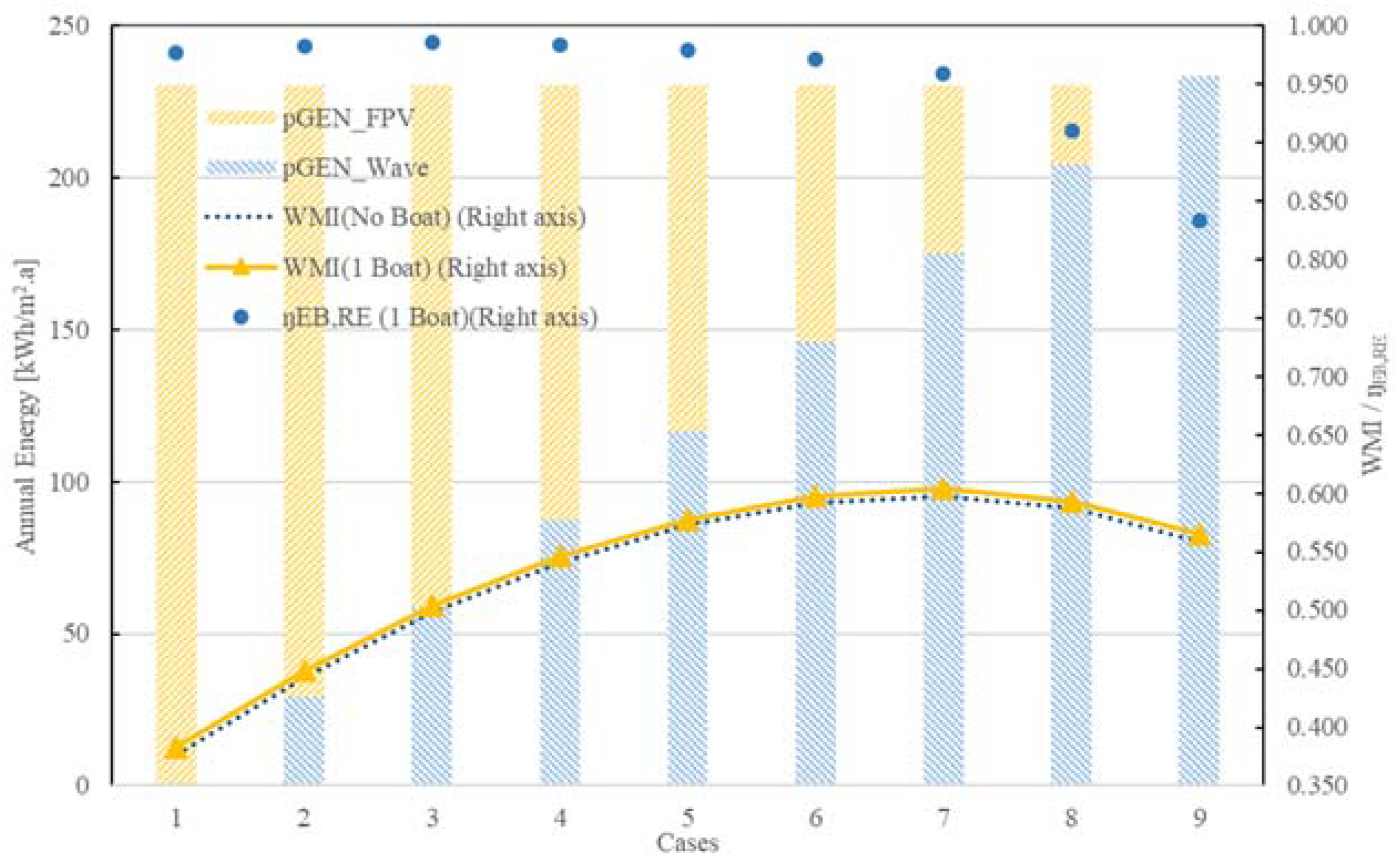
5.2.1. The Impact of the Combined Wave-FPV Energy System on the Technical Performance of the Hybrid System: Mixing Based on Total Generation (Investigation with a Single E-Boat)

Table 4. The options of variables in Scenario 1, combination cases are based on the same total generation.

	Variables	Options of the Variables
	Case		1	2	3	4	5	6	7	8	9
Scenario 1	On-Site ORE	WEC [Unit]	0	5	10	15	20	25	30	35	40
		FPV [m2]	5524.5	4834.7	4124.6	3425.4	2726.3	2027.2	1326.4	627.3	0
	Cruise Velocity	7.5 km/h
	Cruise Distance	10 km
	The number of electric boats	0 or 1
	With building to boat function	Yes
	With boat-to-building function	No

shows the groups investigated in this section. There are nine different combinations with two ocean renewable energy systems, and these mixed combinations are based on the same total generation required to meet the total annual electricity demand of the building (approximately 230.27 kWh/m².a). In other words, all cases, from Case 1 to Case 9, are able to generate the same amount of renewable energy required to support the hotel building. The cruising velocity and distance are fixed at 7.5 km/h and 10 km for ease of comparison between cases without and with an electric boat.

Figure 9 and Table 4 illustrate the simulation results of annual energy generation, REe matching capacity, and CO₂ emissions for Scenario 1. It can be seen that as the number of WECs increases from 0 to 40 units (corresponding to a decrease in the area of the applied FPV), the dashed line represents the WMI of the combination group without boat, which exhibits an increase from 0.376 to 0.592, and a continuous decrease in WMI from group 7 to 9 (0.598 to 0.559). It can be seen that when no electric boat is included in the hybrid system, with 30 units of WEC and 1326.4 m² of FPV (Case 7), the highest degree of matching between the whole Wave-FPV system and the energy consumption of the building is achieved. This means that when the combined ORE system presented in Case 7 is applied, the annual exported REe (86.85 kWh/m²) and imported grid electricity (98.36 kWh/m²) are the lowest among the nine cases. The total annual energy generation ratio of WEC and FPV are 76% and 24%, respectively. The yellow line in Figure 9 shows the simulation results of WMI when one electric boat is applied in the Wave-FPV hybrid system. The trend of change is consistent with the absence of electric boats, and Case 7 still provides the best matching ability among these cases (with a WMI of 0.603). However, when considering the interaction with the E-boat, the exported on-site REe decreases, because the E-boat requires energy support from the surplus REe while moored. When the E-boat is moored, the energy generated by the PV of the E-boat will be prioritized for use in supporting the building, resulting in the amount of imported grid electricity also being reduced. WMI is the overall REe matching index, and compared with the scenario without a boat, the WMI of the scenario with a boat also increases slightly, and the WMI of each combination of cases increases by between 0.9 and 1.8%.

Another coefficient of interest is the annual local renewable energy ratio in the electric boat integrated system (${“\mathsf{\eta }}_{\mathrm{EB},\mathrm{RE}}”$), which is shown in Figure 9 with blue dots. As illustrated, this ratio reaches a maximum value (0.985) in Case 3, then decreases to 0.833 as the number of WEC units increases. This coefficient (${“\mathsf{\eta }}_{\mathrm{EB},\mathrm{RE}}”$) converges to 1, which means that the E-boat consumes more on-site REe and relies less on the nighttime grid to replenish the battery. The reason for this is that when the Wave-FPV hybrid system applies more WEC to generate electricity, the nighttime mandatory charging mode will be activated due to the REe being insufficient to replenish the battery during the daytime while docked at the shore, leading to a decrease in the annual local renewable energy ratio. Therefore, Case 3 has a better combination of generators for supporting daily E-boat cruises.

In

Table 5. The annual energy, matching capabilities, and emissions of the 3 representative cases in Scenario 1 (the bolded and underlined values are the best values in this scenario).

Scenario 1
Cases	Case 1 (Only FPV)		Case 7 (Mixing)		Case 9 (Only WEC)
	without Boat	with Boat	without Boat	with Boat	without Boat	with Boat
Eimp,a [kWh/m2.a]	149.51	149.46	98.36	98.15	106.60	106.33
Eexp,a [kWh/m2.a]	138.04	137.29	86.85	85.91	97.97	96.99
Edirect,a [kWh/m2.a]	11.47	12.20	11.51	12.24	8.63	9.34
OEFe	0.351	0.357	0.573	0.578	0.537	0.543
OEMe	0.401	0.408	0.623	0.629	0.580	0.587
WMI	0.376	0.382	0.598	0.603	0.559	0.565
ŋEB,RE	-	0.977	-	0.959	-	0.833
CEa [kg CO2,eq/m2.a]	5.57	5.93	5.59	5.95	4.19	4.54

, the three most representative sets of results are shown. Case 1 has only the FPV system (5524.5 m²), Case 7 has 30 units of WECs and 1326.4 m² of FPV, and Case 9 has 40 units of WECs only. It can be seen that the WMI (0.376) is the worst when only the FPV system is applied, with a high volume of imported and exported energy. When the WEC is introduced into the hybrid ORE system, the mismatching between renewable energy and the building is improved. Similarly, when only WEC is applied, this combination case can also cause an energy mismatching issue. The WMI of Case 9 is only 0.559, which is not the highest among the groups. Therefore, the conclusion is that the use of a Wave-FPV mixture could improve the mismatching issue of on-site REe. It is worth mentioning that when an E-boat interacts with the building, the PV of the boat is able to provide REe to the hotel building when the boat is docked, and when the on-site REe is in surplus, the battery of the boat can be charged. Therefore, the “E_imp,a” and “E_exp,a” of those cases with a boat are all lower than the cases without a boat, leading to a better WMI as a result. For example, in Case 7, the WMI is increased from 0.598 to 0.603 due to the participation of the E-boat. Although both the “E_imp,a” and the “E_exp,a” are decreasing at the same time due to the application of the E-boat, the “E_direct,a” does not decrease, but rather increases, and then the amount by which the “E_exp,a” decreases is roughly the same as the amount by which the “E_imp,a” decreases due to the addition of the E-boat. In Case 7, the “E_imp,a” (case without boat) is 98.36 kWh/m².a, the “E_imp,a” (case with boat) is 98.15 kWh/m².a, a decrease of 0.21 kWh/m².a, and the corresponding “E_exp,a” decreases from 86.85 kWh/m².a to 85.91 kWh/m².a, a reduction of 0.94 kWh/m².a. Thus, in Case 7, the annual net direct energy (“E_direct,a”) increases from 11.51 kWh/m².a to 12.24 kWh/m².a. Furthermore, the “CE_a”, the annual equivalent CO₂ emissions of the hybrid system, is directly related to the value of “E_direct,a”. Case 9 without E-boat interaction achieves the lowest CO₂ emissions (4.19 kg CO_2,eq/m².a). Due to the excess size of Case 9, the total annual generation in this case is 3 kWh/m².a higher than the building demand required to keep an integer multiple of the WEC unit. This is the main reason that the values of “E_direct,a” and “CE_a” are the lowest in this case.

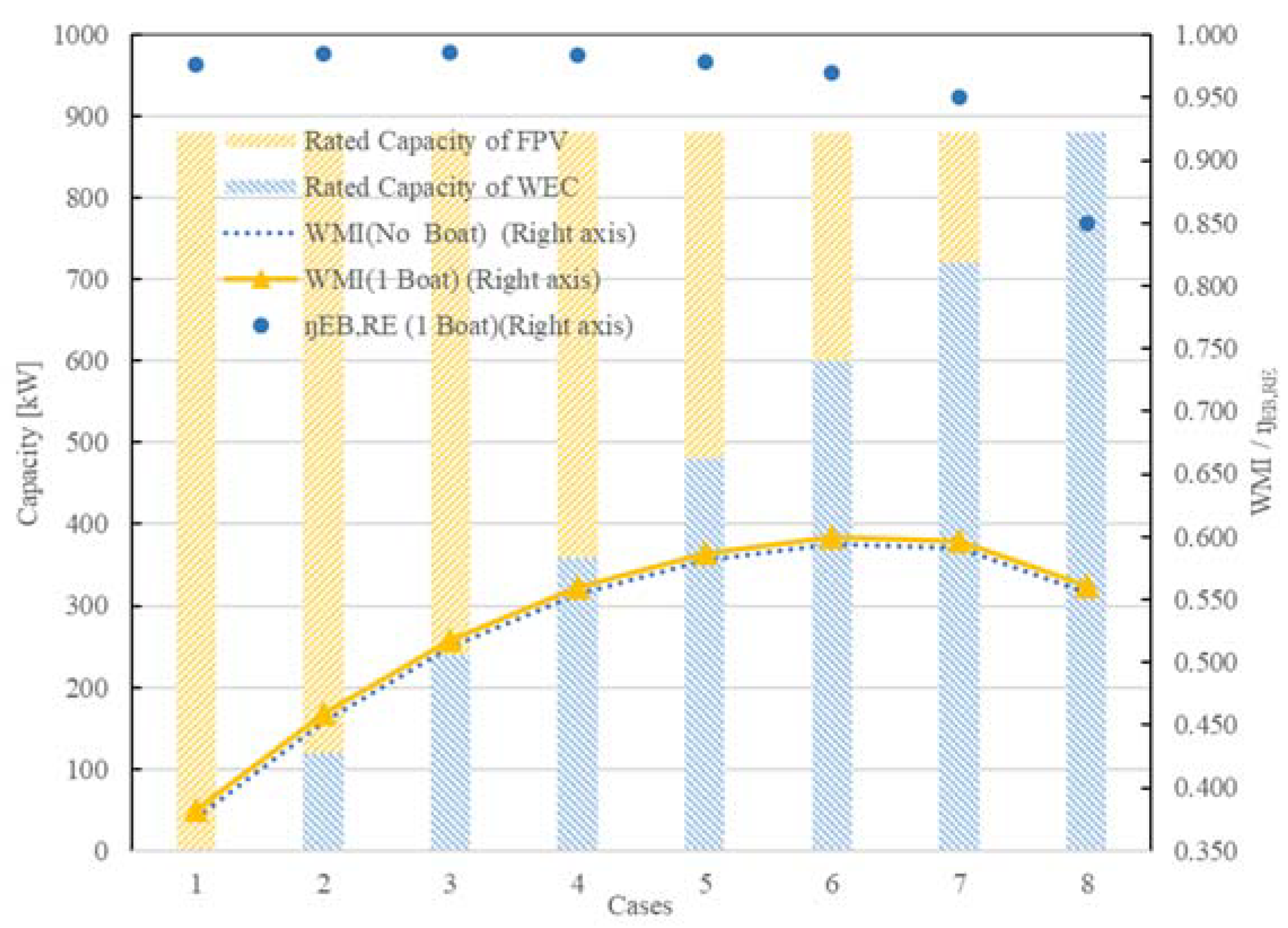
5.2.2. The Impact of the Combined Wave-FPV Energy System on the Technical Performance of the Hybrid System: Mixing Based on Total Rated Capacity (Investigation of a Single E-Boat)

In this sub-section, another eight combination ORE cases will be investigated, as shown in

Table 6. Options of variables in Scenario 2; combination cases are based on the same total rated capacity.

	Variables	Options of the Variables
	Case		1	2	3	4	5	6	7	8
Scenario 2	On-Site ORE	WEC [Unit]	0	6	12	18	24	30	36	44
		FPV [m2]	5528.8	4774.8	4020.9	3267.0	2513.1	1759.2	1005.2	0
	Cruise Velocity	7.5 km/h
	Cruise Distance	10 km
	The number of electric boats	0 or 1
	With building to boat function	Yes
	With boat-to-building function	No

. The mixed cases are based on the same total rated capacity (880 kW). This means that, from Case 1 to Case 8, the total rated capacity of the sum of FPV and WEC remains constant at 880 kW. Similar to in Section 5.2.1, the cruising velocity and distance are fixed at 7.5 km/h and 10 km for ease of comparison between without and with an electric boat.

In Figure 10, the bars indicate the capacity of the corresponding generation system, with yellow bars representing the FPV system, with mix share decreasing from 100% to 0% (from Case 1 to Case 8), with a reduction of 120 kW for each successive case. On the other hand, the blue bars represent the WEC system, increasing by 120 kW per case, until a pure WEC system of 840 kW is applied in Case 8. The dashed line stands for the WMI without boat interaction. As can be seen from Figure 10, this dashed curve gradually decreases again after reaching a maximum at Case 6 (WMI = 0.595). The yellow line represents the case with the participation of one E-boat. The WMI trend is the same, but the WMI in each case is increased by about 0.9–1.8% compared to the reference case without the E-boat. With respect to the “${\mathsf{\eta }}_{\mathrm{EB},\mathrm{RE}}$”, which is the annual local renewable energy ratio in the E-boat integrated system, in Scenario 2, the highest value occurs in Case 3, with a value of around 0.986. In other words, only 2% of the energy is supplied by the grid in throughout a whole year. All other cases exhibited decreased “${\mathsf{\eta }}_{\mathrm{EB},\mathrm{RE}}$”, and it is worth noting that when only WEC is applied to provide REe, the matching between E-boat and REe is the worst (0.850), again indicating that the WEC system generates energy with greater uncertainty and instability. Section 5.2.3, below, will evaluate the uncertainty and instability of REe generation by showing and analyzing the annual monthly data and daily profile.

In Scenario 2, as shown in

Table 7. The annual energy, matching capabilities, and emissions of the 3 representative cases in Scenario 2 (the bolded and underlined values are the best values in this scenario).

Scenario 2
Cases	Case 1 (Only FPV)		Case 6 (Mixing)		Case 8 (Only WEC)
	without Boat	with Boat	without Boat	with Boat	without Boat	with Boat
Eimp,a [kWh/m2.a]	149.49	149.44	94.14	93.98	101.62	101.34
Eexp,a [kWh/m2.a]	138.20	137.41	99.77	98.88	115.15	114.17
Edirect,a [kWh/m2.a]	11.30	12.03	−5.63	−4.90	−13.53	−12.83
OEFe	0.351	0.357	0.591	0.596	0.559	0.564
OEMe	0.400	0.408	0.598	0.604	0.551	0.558
WMI	0.376	0.382	0.595	0.600	0.555	0.561
ŋEB,RE	-	0.977	-	0.970	-	0.850
CEa[kg CO2,eq/m2.a]	5.49	5.85	−2.74	−2.38	−6.58	−6.23

, three representative cases are selected to demonstrate several important technical indexes. It can be seen that Case 6 has the best on-site REe matching ability; regardless of whether the E-boat interacts with the building or not, Case 6 always has the lowest values of “E_imp,a” and “E_exp,a”, and the best values of OEFe, OEMe, and WMI, thus making it the best among the eight cases. In Case 6, without E-boat interaction, WMI reaches a value of 0.595. In the case of the application of E-boat, the WMI is 0.600. In particular, since the combined ORE system in this scenario is based on the same total rated capacity, in accordance with this condition, all the combination cases of the ORE system will generate more REe than the electricity demand of the hotel building. In accordance with the energy management strategies described in Section 2.1, the surplus REe will be prioritized for use in charging the E-boat. If there is still any remaining surplus, the remainder of the REe will be fed into the grid. This will result in the cases with more WEC beingn better equipped, and thus generating more REe. When “E_imp,a” is lower than “E_exp,a”, the “E_direct,a” will have a negative value. Therefore, Case 8 without any E-boat interaction achieves the lowest CO₂ emissions (−6.58 kg CO_2,eq/m².a).

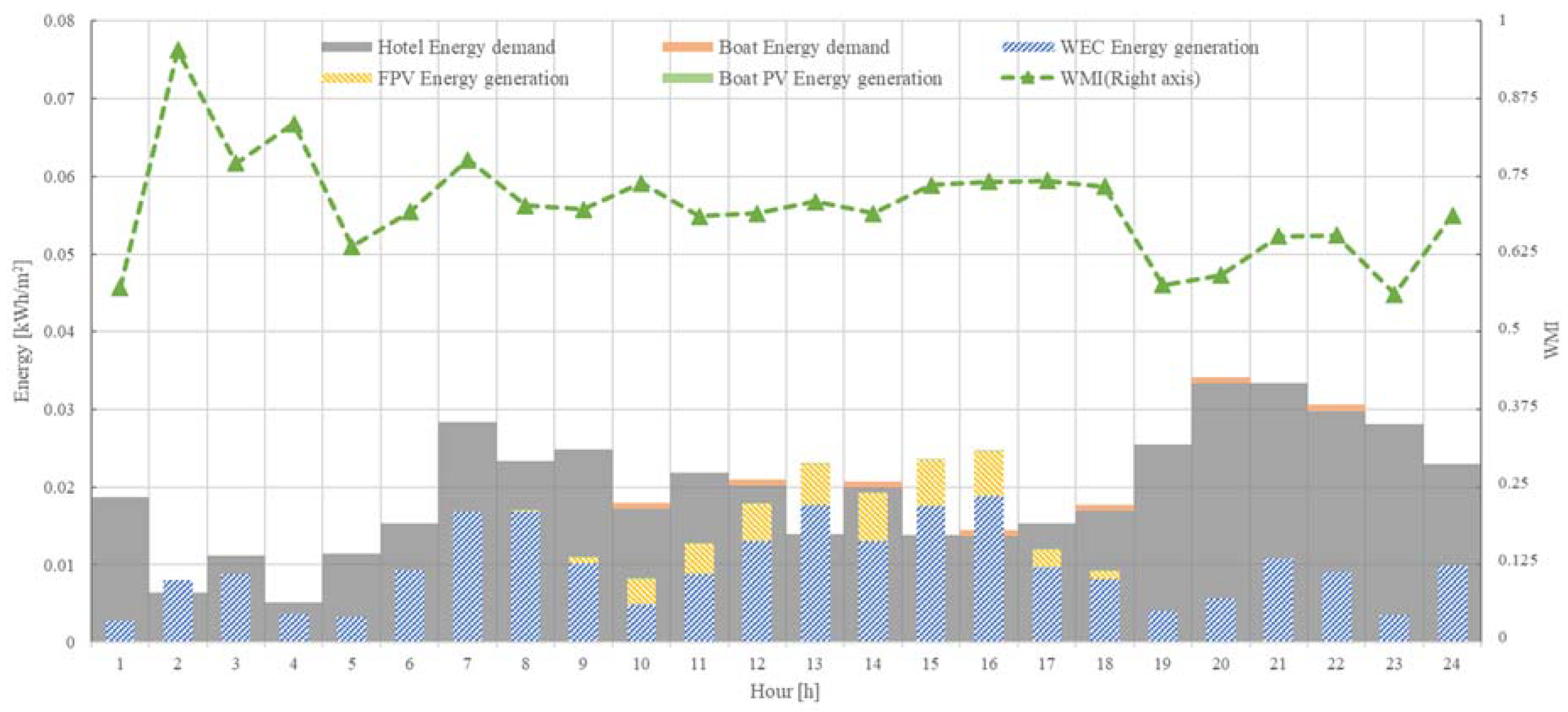
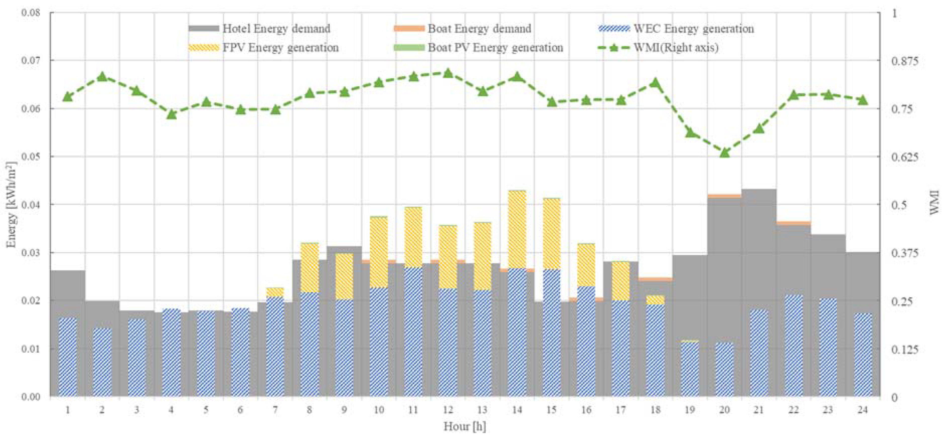
5.2.3. The Monthly and Hourly Technical Performance of the Combined Wave-FPV Energy System (Investigation of a Single E-Boat)

Figure 11 shows the total energy generation per month when equipped with 30 units of WECs and 1759.3 m² FPV to help better understand the technical performance of the hybrid ORE system. The graph also illustrates the monthly energy demand for the hotel and the E-boat. It is reported that the monthly energy consumption of the hotel building is much higher than that of the E-boat. The average monthly energy consumption of the building is between 8 and 31 kWh/m², with February having the lowest energy demand, at 7.9 kWh/m², and November having the highest in the year, reaching 32.83 kWh/m². However, the annual renewably generated energy is already 248.31 kWh/m² under this hybrid system, far exceeding the annual demand of 232.21 kWh/m² for the hotel and the E-boat. However, there is a severe shortage of REe from February to June and in October. The REe during these months is very low mainly because of the poor generation performance of WEC. During these months, the shortages will be supported by the grid. At the same time, the WMI is not high due to the heavy reliance on the grid. For example, the WMI from February to April, and in October and December, are all below 0.6, indicating that the energy generated on site does not match well with the energy demand of the building. To explain in more detail the fluctuations of the WMI and technical performance of the hybrid REe system, the tenth days of February and June are chosen for comparison, as shown in Figure 12 and Figure 13. The 10 February (daily average WMI of 0.64) is shown as a typical REe short day. The 10 June (daily average WMI of 0.74) is shown as a general day.

On the one hand, it can be observed from this comparison that the daily building demand in June in summer (0.65 kWh/m²) is 1.4 times higher than in February in winter (0.48 kWh/m²). The REe values of the same day are 0.60 kWh/m² and 0.27 kWh/m², respectively. While energy demand is higher in summer than in winter, total renewable energy generation is also higher in summer than in winter—about twice as much as in winter. Another aspect, in both summer and winter, is that there are two peaks in building energy demand, one from 8:00 to 14:00 and one from 20:00 to 1:00. In the summer, with plenty of solar radiation, it is possible to cover the morning to midday power peaks, which is the reason the WMI continues to remain high during this period (above 0.75), while in the winter, the WMI during the same period is a bit worse (0.7–0.75), it still could receive benefit from FPV. Nighttime peaks are a significant problem in summer and winter when nighttime waves are not good enough. Especially in February, the matching loss of solar energy causes a constant REe deficit.

5.3. The Impact of Electric Boats on the Hybrid Zero-Emission System

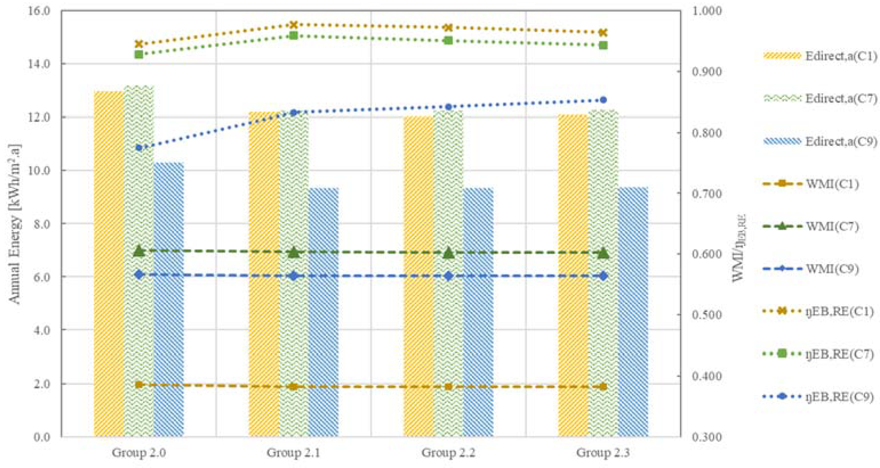
5.3.1. The Impact of the Cruise Velocity and Cruise Distance on the Technical Performance of the Hybrid System (Investigation of a Single E-Boat)

Section 5.2.1 and Section 5.2.2, above, investigated the technical performance of the E-boat at a fixed cruising velocity and distance for different cases of the combination of two ORE systems. According to the product datasheet provided by the E-boat manufacturer, it is known that the energy demand of the boat is different at different velocities. In the following sections, as shown in

Table 8. The simulation groups and variables of different E-boat cruise velocities.

Simulation Groups	with 1 Boat	with Building to Boat Function	with Boat-to-Building Function	Cruise Distance [km]	Cruise Velocity [km/h]
Group 2.0	Yes	Yes	No	7.5	15
Group 2.1	Yes	Yes	No		10
Group 2.2	Yes	Yes	No		7.5
Group 2.3	Yes	Yes	No		6

, the technical effects of Scenario A, consisting of four different cruising velocities (6, 7, 10 and 15 km/h, respectively) at the same cruising distance (7.5 km), and Scenario B, consisting of four different distances (5, 7.5, 10 and 12.5 km, respectively) at the same velocity (10 km/h), on the hybrid system are discussed. All of the groups in these two scenarios only possess the building-to-boat function. The boat-to-building function is not activated.

• Cruise velocity as the variable (Scenario A)

For each group, as shown in Figure 14 and

Table 9. Comparison of annual energy, matching capability and emissions among different cruising velocity groups (the bolded and underlined values are the best values in this scenario).

Simulation Groups	Selected Cases	Edirect,a [kWh/m2.a]	WMI	${\mathsf{\eta }}_{\mathbf{EB}\mathbf{,}\mathbf{RE}}$	CEa [kg CO2,eq/m2.a]
Group 2.0 (Velocity 15 km/h)	C1	12.963	0.385	0.945	6.300
	C7	13.176	0.606	0.928	6.404
	C9	10.397	0.567	0.775	5.005
Group 2.1 (Velocity 10 km/h)	C1	12.204	0.382	0.977	5.931
	C7	12.239	0.603	0.959	5.948
	C9	9.340	0.565	0.833	4.539
Group 2.2 (Velocity 7.5 km/h)	C1	12.040	0.382	0.972	5.851
	C7	12.240	0.603	0.951	5.949
	C9	9.336	0.564	0.842	4.537
Group 2.3 (Velocity 6 km/h)	C1	12.075	0.382	0.964	5.868
	C7	12.271	0.603	0.943	5.964
	C9	9.371	0.564	0.853	4.554

, instead of presenting nine Wave-FPV generation system combination cases, only three cases are selected on the basis of the same total energy generation, in order to provide clear and comparable results. C1 (Case 1) is only equipped with FPV (around 5524.5 m²), while C8 is only equipped with 31 units of WEC, while C7 is a hybrid system with 30 units of WEC and 1326.4 m² of FPV. From Group 2.0 to Group 2.3, the E-boat cruise velocity decreases in order, from 15 km/h to 6 km/h. Among these groups, “Group 2.0 (C7)” shows the best matching ability, with a WMI of 0.606, and the highest values of “E_direct,a” and “CE_a”, which are 13.176 kWh/m².a and 6.404 kg CO_2,eq/m².a, respectively. All of this can be attributed to the fact that the faster the boat travels over the same distance, the more the demand for the boat will increase, while also providing more mooring time in the port, and the building can provide more surplus REe to the boat. “Group 2.1 (C1)” has the maximum “ŋ_EB,RE” (0.977), meaning that only 2.3% of the boat’s energy demand needs to be sourced from the grid, while 97.7% is entirely supported by REe. The lowest values for “E_direct,a” and “CE_a” occurred in “Group 2.2 (C9)”, with values of 9.336 kWh/m².a and 4.537 kg CO_2,eq/m².a, respectively. Since the entire loadout for “C9” consists of 40 units of WECs as the only generation system, and since the number of devices should always be an integer, in this case, the total generation energy is slightly higher than the total energy demand, meaning that there will be more energy exported to the grid, resulting in the minimization of “E_direct,a” and “CE_a”.

It is worth mentioning that, for the same case, for example, “Group 2.0 (C7)” has the WMI with the highest value, which is 0.606, because this group has the maximum velocity. In “Group 2.1 (C7)”, “Group 2.2 (C7)”, “Group 2.3 (C7)”, the WMI (0.603) of these three groups remains almost unchanged even when decreasing the cruising velocity from 10 km/h to 6 km/h. The “E_direct,a” and “CE_a” slightly increase when decreasing the cruising velocity from 15 km/h to 6 km/h in the same case. “Group 2.3 (C7)” has the worst “E_direct,a” and “CE_a” among these three groups, with values of 12.271 kWh/m².a and 5.964 kg CO_2,eq/m².a, respectively. This is because when the velocity is reduced to its lowest value, the sailing time increases, and the possible time moored in port becomes shorter, reducing the time that the boat can interact with the building, resulting in the boat not being able to use the surplus REe. At the same time, the building cannot use boat PV generation to cover energy shortages, leading to an increase in imported electricity; thus, “Group 2.3” possesses the highest values of “E_direct,a” and “CE_a” among the three groups. Case 7 always exhibts the highest “E_direct,a” and “CE_a” in its group, because this case has lower values of “E_imp,a” and “E_exp,a”, allowing a better energy matching ability. Therefore, the annual net direct energy and the operational equivalent CO₂ emissions can be kept at higher values than those in Case 1 and 9.

2.

Cruise distance as the variable (Scenario B)

In Scenario B, as reported in

Table 10. The simulation groups and variables of different E-boat cruise distances.

Simulation Groups	With 1 Boat	With Building to Boat Function	With Boat-to-Building Function	Cruise Distance [km]	Cruise Velocity [km/h]
Group 2.4	Yes	Yes	No	5	10
Group 2.1	Yes	Yes	No	7.5
Group 2.5	Yes	Yes	No	10
Group 2.6	Yes	Yes	No	12.5

, there are four groups under investigation. The cruise velocity is fixed at 10 km/h, and the cruise distance increases from 5 km to 12.5 km, with an increase of 2.5 km for each group. With the velocity remaining constant, the increased distance travelled also means that the sailing time becomes longer. It can be seen in Figure 15 that with increased travel distance, “E_direct,a” also increases significantly, and WMI will also be slightly elevated. The slight increases due to the boat’s demand simultaneously become more significant due to the longer cruising distance, and more surplus REe will be used to charge the boat, resulting in less surplus REe being exported to the grid. However, the increased energy consumption of the boat also makes the boat more dependent on the grid for charging at night to ensure normal cruising activities the next day, and therefore, ${“\mathsf{\eta }}_{\mathrm{EB},\mathrm{RE}}”$ decreases significantly with increasing distance travelled.

In

Table 11. Comparison of annual energy, matching capability and emissions among different cruise distance groups (the bolded and underlined values are the best values in this scenario).

Simulation Groups	Selected Groups	Edirect,a [kWh/m2.a]	WMI	${\mathsf{\eta }}_{\mathbf{EB},\mathbf{RE}}$	CEa [kg CO2,eq/m2.a]
Group 2.4 (Distance 5 km)	C1	10.9	0.378	0.971	5.300
	C7	11.1	0.600	0.991	5.399
	C9	8.2	0.562	0.942	3.987
Group 2.1 (Distance 7.5 km)	C1	12.2	0.382	0.977	5.931
	C7	12.2	0.603	0.959	5.948
	C9	9.3	0.565	0.833	4.539
Group 2.5 (Distance 10 km)	C1	13.7	0.386	0.826	6.641
	C7	13.9	0.607	0.856	6.741
	C9	11.0	0.567	0.747	5.337
Group 2.6 (Distance 12.5 km)	C1	15.8	0.388	0.657	7.668
	C7	16.0	0.610	0.762	7.774
	C9	13.1	0.570	0.697	6.374

, it can be seen that “Group 2.6 (C7)” possesses the maximum WMI (0.610) within these 12 groups, and “Group 2.4 (C7)” has the highest ${“\mathsf{\eta }}_{\mathrm{EB},\mathrm{RE}}”$ (0.991), which indicates that 99.1% of the energy that is used to support the boat comes from REe. “Group 2.4 (C9)” has the lowest “E_direct,a” and “CE_a”, with values of 8.2 kWh/m².a and 3.987 kg CO_2,eq/m².a, respectively. This is because it possesses the shortest cruise distance, which has the lowest boat energy demand and the greatest interaction time with building among the four groups.

5.3.2. The Impact of Boat Battery Capacity and Cruise Patterns on the Technical Performance of the Hybrid System (Investigation of Multiple E-Boats)

In this section, more E-boats will be applied in interaction with the building, and the boat-to-building function will be activated using the same control strategy as described in Section 3.1, which means that when the boats are docked in the harbor, a boat’s batteries are available for discharge to support the building in case of power shortage. On the basis of Section 5.3.1, in this section, all groups are observed only for the hybrid renewable energy system described in Case 7 (WEC of 30 units, FPV of 1326.4 m²) for the other variables. The number of boats in each group is increased from one to eight, and then to 16 in order to investigate energy matching ability, which could potentially be improved in the limit case. The other four groups, Group 3.0 to Group 3.3, have the boat-to-building function activated, and the rest of the variables are the same as in Group 2.0 to Group 2.3.

Table 12. The simulation groups and variables for the number of E-boats, without and with the boat-to-building function and at different cruise velocities.

Simulation Groups	The Number of Boats	With Building to Boat Function	With Boat-to-Building Function	Cruise Distance	Cruise Velocity
				[km]	[km/h]
Group 2.0	1–8, 16	Yes	No	7.5	15
Group 2.1	1–8, 16	Yes	No		10
Group 2.2	1–8, 16	Yes	No		7.5
Group 2.3	1–8, 16	Yes	No		6
Group 3.0	1–8, 16	Yes	Yes	7.5	15
Group 3.1	1–8, 16	Yes	Yes		10
Group 3.2	1–8, 16	Yes	Yes		7.5
Group 3.3	1–8, 16	Yes	Yes		6

shows details. The maximum number of boats for hotel tourist usage is eight. Sixteen boats are proposed as the extreme case in order to investigate the improvability of WMI. An economic evaluation of increased interaction boats will be performed in Section 5.4.2.

• Cruise velocity as the variable

In Figure 16a,b, it can be seen that “E_direct” is increases continuously with increasing number of boats, with the most significant changes being in Group 2.0 and Group 3.0. WMI also continues to increase as with increasing number of boats, the along with increasing boat battery capacity, and an increase in the support and interaction that the building can potentially receive from the boats. Specifically, when the boat-to-building function is activated in Group 3.0 to Group 3.3, the improvement in WMI is more prominent. Correspondingly, the disadvantage is that “${\mathsf{\eta }}_{\mathrm{EB},\mathrm{RE}}$” continues to decrease with more frequent interaction between increased numbers of boats the building, also leading to an increase in the dependence of boats on the grid.

It can be seen that the best WMI groups are Group 2.0 and Group 3.0, which reach a WMI of 0.680 and 0.703 with 16 boats, due to their cruise velocity of 15 km/h, which increases the energy consumption of the boats, but also provides more time for the boats and the building to interact. It is also known that activating the boat-to-building function improves the overall WMI by about 2–3%. The interaction of more boats, while enhancing the matching ability of the on-site REe with the building, is not beneficial for other indexes, as can be seen in

Table 13. The annual energy, matching capability and emissions among different cruise velocity groups without the boat-to-building function (The bolded and underlined values are the best results in this scenario).

Simulation Groups	The Number of Boats	Edirect,a [kWh/m2.a]	WMI	${\mathbf{\eta }}_{\mathbf{E}\mathbf{B},\mathbf{R}\mathbf{E}}$	CEa [kg CO2,eq/m2.a]
Group 2.0 (Velocity 15 km/h)	1	13.176	0.606	0.928	6.404
	8	24.861	0.649	0.817	12.083
	16	38.204	0.680	0.745	18.567
Group 2.1 (Velocity 10 km/h)	1	12.239	0.603	0.959	5.948
	8	17.320	0.635	0.874	8.417
	16	23.047	0.661	0.816	11.201
Group 2.2 (Velocity 7.5 km/h)	1	12.240	0.603	0.951	5.949
	8	17.299	0.633	0.862	8.407
	16	22.971	0.658	0.800	11.164
Group 2.3 (Velocity 6 km/h)	1	12.271	0.603	0.943	5.964
	8	17.544	0.631	0.844	8.526
	16	23.467	0.655	0.785	11.405

and

Table 14. The annual energy, matching capability and emissions among different cruise velocity groups with the boat-to-building function (The bolded and underlined values are the best results in this scenario).

Simulation Groups	The Number of Boats	Edirect,a [kWh/m2.a]	WMI	${\mathbf{\eta }}_{\mathbf{E}\mathbf{B},\mathbf{R}\mathbf{E}}$	CEa [kg CO2,eq/m2.a]
Group 3.0 (Velocity 15 km/h)	1	12.892	0.627	0.886	6.266
	8	24.839	0.680	0.730	12.072
	16	38.715	0.703	0.664	18.815
Group 3.1 (Velocity 10 km/h)	1	11.846	0.624	0.894	5.757
	8	16.814	0.673	0.747	8.171
	16	23.261	0.694	0.685	11.305
Group 3.2 (Velocity 7.5 km/h)	1	11.797	0.622	0.885	5.733
	8	16.707	0.669	0.732	8.119
	16	22.978	0.689	0.666	11.167
Group 3.3 (Velocity 6 km/h)	1	11.785	0.619	0.873	5.728
	8	16.711	0.664	0.718	8.122
	16	23.198	0.684	0.651	11.274

and Figure 16, where Group 2.1 (cruise velocity is 10 km/h) with only one boat possesses both the minimum “E_direct” and “CE_a” and the highest “${\mathsf{\eta }}_{\mathrm{EB},\mathrm{RE}}$”, with values of 12.239 kWh/m².a, 5.948 kg CO_2,eq/m².a, and 0.959, respectively. Group 3.1, with a cruising velocity of 10 km/h when the boat-to-building function is activated, still has the highest “${\mathsf{\eta }}_{\mathrm{EB},\mathrm{RE}}$” (0.894), but the lowest “E_direct” (11.785 kWh/m².a) and “CE_a” (5.728 kg CO_2,eq/m².a) were found in Group 3.3 (cruising velocity of 6 km/h with 1 boat).

2.

Cruise distance as the variable

This section will continue to investigate the effect of progressively increasing the number of boats with and without the boat-to-building function on the technical performance of the overall hybrid system. The variables are listed in

Table 15. The simulation groups and variables of the number of E-boats, with the boat-to-building function and different cruise distances.

Simulation Groups	The Number of Boats	With Building to Boat Function	With Boat-to-Building Function	Cruise Distance	Cruise Velocity
				[km]	[km/h]
Group 2.4	1–8, 16	Yes	No	5	10
Group 2.1	1–8, 16	Yes	No	7.5
Group 2.5	1–8, 16	Yes	No	10
Group 2.6	1–8, 16	Yes	No	12.5
Group 3.4	1–8, 16	Yes	Yes	5	10
Group 3.1	1–8, 16	Yes	Yes	7.5
Group 3.5	1–8, 16	Yes	Yes	10
Group 3.6	1–8, 16	Yes	Yes	12.5

.

First of all, except for Group 2.4 and Group 3.4, which have the shortest cruise distance (5 km) among all of the groups, meaning that the boat is able to stay in port for longer periods of time, the “E_direct” decreases when the number of boats increases. For the other groups, longer cruise distances and greater numbers of interacting boats lead to a continual increase in “E_direct”. Secondly, in the groups in which the boat-to-building function is not activated, it is easy to understand that the longer the sailing distance and the greater the number of participating boats, the higher the WMI will be. Because the energy demand of the boats will increase, more REe will be used. Therefore, the maximum WMI (0.678) is encountered in Group 2.5 with 16 boats. However, after activating the boat-to-building function, the distance travelled does not significantly change, although the WMI value increases with the number of boats. It is not until the number of boats reaches 16 that the maximum value of WMI 0.694 appears in Group 3.1. Thirdly, it can be seen from Figure 17a,b that as the number of boats increases and the distance travelled increases, “${\mathsf{\eta }}_{\mathrm{EB},\mathrm{RE}}$” continuously decreases. The reason for this is that increasing the distance and the number of boats also increases the total boat energy demand, and the need for forced charging from the grid at night increases accordingly.

More detailed results are shown in

Table 16. The annual energy, matching capability, and emissions among different cruise distance groups without the boat-to-building function (The bolded and underlined values are the best results in this scenario).

Simulation Groups	The Number of Boats	Edirect,a [kWh/m2.a]	WMI	${\mathsf{\eta }}_{\mathbf{EB}\mathbf{,}\mathbf{RE}}$	CEa@ [kg CO2,eq/m2.a]
Group 2.4 (C7) (Distance 5 km)	1	11.109	0.600	0.991	5.40
	8	8.300	0.615	0.968	4.03
	16	5.063	0.629	0.953	2.46
Group 2.1 (C7) (Distance 7.5 km)	1	12.239	0.603	0.959	5.95
	8	17.320	0.635	0.874	8.42
	16	23.047	0.661	0.816	11.20
Group 2.5 (C7) (Distance 10 km)	1	13.871	0.607	0.856	6.74
	8	30.386	0.650	0.714	14.77
	16	49.178	0.678	0.628	23.90
Group 2.6 (C7) (Distance 12.5 km)	1	15.996	0.610	0.762	7.77
	8	47.403	0.656	0.568	23.04
	16	83.194	0.673	0.455	40.43

and

Table 17. The annual energy, matching capability, and emissions among different cruise distance groups with the boat-to-building function (the bolded and underlined values are the best results in this scenario).

Simulation Groups	The Number of Boats	Edirect,a [kWh/m2.a]	WMI	${\mathsf{\eta }}_{\mathbf{EB}\mathbf{,}\mathbf{RE}}$	CEa [kg CO2,eq/m2.a]
Group 3.4 (C7) (Distance 5 km)	1	10.773	0.625	0.928	5.24
	8	7.783	0.673	0.810	3.78
	16	5.553	0.692	0.749	2.70
Group 3.1 (C7) (Distance 7.5 km)	1	11.846	0.624	0.894	5.77
	8	16.814	0.673	0.747	8.32
	16	23.261	0.694	0.685	11.36
Group 3.5 (C7) (Distance 10 km)	1	13.518	0.623	0.849	6.54
	8	30.169	0.672	0.661	14.64
	16	49.239	0.692	0.578	23.93
Group 3.6 (C7) (Distance 12.5 km)	1	15.587	0.622	0.779	7.58
	8	47.119	0.667	0.573	22.90
	16	83.177	0.677	0.466	40.42

. Group 2.4 and Group 3.4 have the shortest cruise distance (5 km), meaning that they have the longest interaction time with the building, and the values of “E_direct” and “CE_a” are lowest when 16 boats are involved in the interaction. These are 5.063 kWh/m².a and 5.553 kWh/m².a, 2.46 kg CO_2,eq/m².a and 2.70 kg CO_2,eq/m².a, respectively. Meanwhile, “${\mathsf{\eta }}_{\mathrm{EB},\mathrm{RE}}$” is highest in these two groups when only one boat is involved in the interaction, with values of 0.991 and 0.928, respectively. When considering longer distances as well as increased numbers of boats, the boats become more dependent on the grid, resulting in a constant decline in “${\mathsf{\eta }}_{\mathrm{EB},\mathrm{RE}}$”.

5.4. The Techno-Economic Analysis of the Hybrid Zero-Emission System

5.4.1. The Techno-Economic Analysis for the Integrated Ocean Energy Systems (Investigation of a Single E-Boat)

On the basis of the same simulation groups described in Section 5.2.1, a techno-economic analysis will be performed. In this section, two economic indicators will be evaluated. One is the static economic indicator relative simple payback period (“SPP_rel”), and the other is the dynamic economic indicator relative net present value (“NPV_rel”). The reference capital cost and maintenance cost of the REe system, the electricity cost, and the feed-in-tariff of the REe are listed in

Table 18. The cost profile of the ocean renewable energy hybrid system, boat PV and battery, relative tariff, and exchange rate.

	WEC	FPV	Boat PV	Boat Battery
Capital Cost	45,630 HKD/kW [57]	26,520 HKD/kW [58]	37,331 HKD/kW [59]	1560 HKD/kWh [60]
O&M Cost	4.80%	1.92%	0.86%	/
Electricity Fee	1.22 HKD/kWh [61]
Feed-in-Tariff	3.00 HKD/kWh [62]
Interest Rate	2.139% [55]
USD to HKD Exchange rate	7.80 [63]

. In this study, the cost of the E-boat will not be considered directly. It is assumed that the cost of the E-boat can be compensated for via tourist revenue. Thus, the cost of the boat PV and the boat battery cost will be considered rather than considering the total cost of the boat. In particular, the boat battery will be included in the capital cost of the boat, and according to the datasheet provided by the boat’s manufacturer, a replacement battery will be considered when the number of charge cycles of the boat battery is greater than 2000 cycles.

When there are no boats interacting with the building, the number of WECs in the hybrid ORE system gradually increases (as can be seen from Table 4) from Case 1 until Case 9, which is fully equipped with 40 WECs only. As can be seen from the cost profile shown in Table 18, the capital cost of WEC is 1.72 times higher than that of FPV. This results in a continuous increase in simple payback period from Case 1 to Case 9, from 9.59 years to 26.58 years, as reported in Figure 18 and

Table 19. The relative simple payback period, relative net present value, matching capability and emissions of the 3 representative cases in Scenario 1 (the bolded values are the best results in this scenario, “FiT” is the feed-in-tariff, “BLT” is an abbreviation for beyond the lifetime).

	Group	Variables	SPPrel (without FiT)	SPPrel (with FiT)	NPVrel (Million HKD)	WMI	CEa [kg CO2,eq/m2.a]
Scenario 1	Case 1 (Only FPV)	Without Boat	BLT	9.59	16.04	0.376	5.57
		With Boat	BLT	9.63	16.15	0.382	5.93
	Case 5 (Mixing)	Without Boat	BLT	14.87	2.54	0.572	5.57
		With Boat	BLT	14.85	2.65	0.578	5.93
	Case 9 (Only WEC)	Without Boat	BLT	26.58	−14.42	0.559	4.19
		With Boat	BLT	26.35	−14.30	0.565	4.54

. Meanwhile, the NPV_rel over the 20-year life cycle drops from a profit of HKD 16.04 million to a loss of HKD 14.42 million. This also indicates that the static indicator of the simple payback year shows that in Case 6 the investment cost can be recovered within 16.9 years. However, with the dynamic indicator, the NPV_rel, of Case 6, it is impossible to recover the investment cost in 20 years. Compared to the static indicator, the dynamic indicator allows for a fine-grained and meaningful comparison of the economic benefits of different hybrid systems. As for the emissions, “CE_a” did not vary significantly from Case 1 to Case 9, reaching a minimum value of 4.19 kg CO_2,eq/m².a in Case 9. WMI reaches its maximum in Case 7 (0.598). It is worth mentioning that Case 5, although not the option with the best return on investment, still has a promising relative simple payback period and positive NPV_rel. These are 14.87 years and HKD 2.54 million, respectively. Case 5 has 20 units of WECs and 2726.3 m² of FPV. When the number of WECs exceeds 20, it is not easy achieve a positive NPV_rel. Although Case 7, with 30 units of WECs and 1326.4 m² FPV, has the most significant technical performance and energy matching capacity, the NPV_rel is already negative.

Moreover, when the E-boat is involved, the boat and the building interact, benefiting both technical and economic aspects. Although the change resulting from one boat is small, compared with Case 5, the simple payback period does not show a significant change, and the NPV_rel is HKD 0.11 million more. This hybrid system (Case 5 with one boat participating) exhibits a better WMI (0.578) while also achieving the profitability of the investment (HKD 2.65 million). It is worth noting that when there is no feed-in-tariff support, either with or without boat involvement, in any combination of renewable energy systems, the initial investment is hard to recover, leading to the simple payback period being consistently negative.

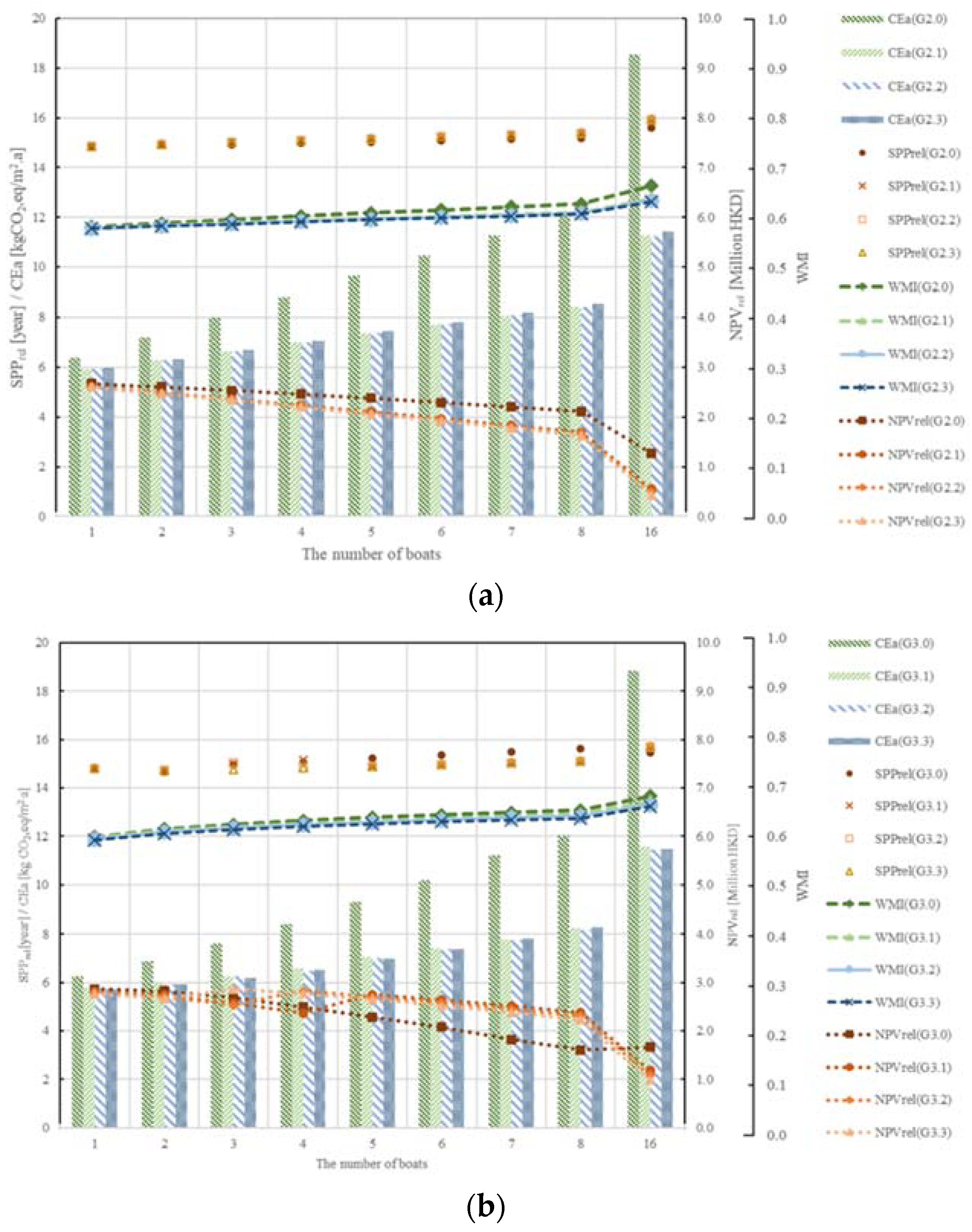
5.4.2. The Techno-Economic Analysis of the Electric Boat Energy Systems (Investigation of More E-Boats)

The comparable groups and cases in this sub-section are the same as those in Section 5.3.2. The variables are reported in Table 12. The compared case is changed to Case 5 rather than Case 7, considering that the combination in Case 7 requires the implementation of 30 units of WEC, which do not easily become profitable over a 20-year life cycle. Therefore, the economic analysis is performed using Case 5 to ensure high WMI and economic feasibility. Moreover, considering the higher WMI occurring in the group with different cruising distances, the group with different cruising distances will not be investigated again in this section. All techno-economic analyses will be performed on the basis of the technical performance of Case 5 to simplify the comparison. This case employed 20 units of WEC and 2726.3 m² of FPV. When the boat-to-building function is not activated, “SPP_rel” is not sensitive to the velocity of the boat, and the values of “SPP_rel” are almost the same for the same number of boats; with increasing number of boats, “SPP_rel” also grows gradually, but it is not very obvious. As shown in Figure 19 and

Table 20. The relative simple payback period, relative net present value, matching capability and emissions of the 3 representative number of E-boats cases among different cruise velocity groups without the boat-to-building function (the bolded and underlined values are the best results in this scenario).

Simulation Groups	The Number of Boats	SPPrel (without FiT)	SPPrel (with FiT)	NPVrel [Million HKD]	WMI	CEa [kgCO2,eq/m2.a]
Group 2.0 (C5) (Velocity 15 km/h)	1	BLT	14.83	2.67	0.580	6.386
	8	BLT	15.19	2.11	0.626	12.068
	16	BLT	15.61	1.28	0.663	18.552
Group 2.1 (C5) (Velocity 10 km/h)	1	BLT	14.85	2.61	0.578	5.933
	8	BLT	15.36	1.69	0.610	8.433
	16	BLT	15.90	0.55	0.637	11.250
Group 2.2 (C5) (Velocity 7.5 km/h)	1	BLT	14.85	2.61	0.577	5.935
	8	BLT	15.38	1.66	0.608	8.435
	16	BLT	15.93	0.49	0.634	11.226
Group 2.3 (C5) (Velocity 6 km/h)	1	BLT	14.86	2.60	0.577	5.951
	8	BLT	15.39	1.63	0.606	8.549
	16	BLT	15.95	0.43	0.631	11.434

and

Table 21. The relative simple payback period, relative net present value, matching capability and emissions of the 3 representative number of E-boats cases among different cruise velocity groups with the boat-to-building function (the bolded and underlined values are the best results in this scenario).

Simulation Groups	The Number of Boats	SPPrel (without FiT)	SPPrel (with FiT)	NPVrel [Million HKD]	WMI	CEa [kgCO2,eq/m2.a]
Group 3.0 (C5) (Velocity 15 km/h)	1	BLT	14.77	2.86	0.599	6.241
	8	BLT	15.63	1.61	0.654	12.038
	16	BLT	15.45	1.67	0.683	18.830
Group 3.1 (C5) (Velocity 10 km/h)	1	BLT	14.80	2.81	0.596	5.787
	8	BLT	15.07	2.38	0.646	8.226
	16	BLT	15.64	1.18	0.671	11.580
Group 3.2 (C5) (Velocity 7.5 km/h)	1	BLT	14.80	2.79	0.595	5.754
	8	BLT	15.10	2.31	0.642	8.172
	16	BLT	15.68	1.09	0.666	11.455
Group 3.3 (C5) (Velocity 6 km/h)	1	BLT	14.82	2.77	0.593	5.725
	8	BLT	15.14	2.23	0.638	8.266
	16	BLT	15.72	0.99	0.661	11.500

, in Group 2.0, when the number of boats is increased from one to eight, “SPP_rel” increases from 14.83 to 15.19 years. However, the values of “NPV_rel” are more sensitive, and better able to show the economic advantages of the hybrid system at different velocities. The NPV of Group 2.0 is consistently the highest, and the greater the number of boats, the more pronounced the advantage this velocity brings compared to the other three groups. For example, when there is only one boat, Group 2.0 and Group 2.3 (the group with the lowest “NPV_rel”) have values of “NPV_rel” of HKD 2.67 million and HKD 2.60 million, respectively; a difference of HKD 0.07 million. When the number of boats is expanded to 16, the difference in “NPV_rel” values increases to HKD 0.85 million. It is noteworthy that all of the groups show that the investment cost can be recovered within 20 years, even for the economically worst group—Group 2.3—with 16 boats, the “SPP_rel” is 15.95 years and the “NPV_rel” is HKD 0.43 million. As for the Group 2.0, which has the best technical performance, when employing 16 boats, the values of WMI, “SPP_rel” and “NPV_rel” are 0.663, 15.61 years and HKD 1.28 million, respectively.

After activating the boat-to-building function, on the basis of Figure 19a,b, it can be seen that the shortest “SPP_rel” drops from 14.83 years in Group 2.0 to 14.77 years in Group 3.0 when employing just one boat, and the “NPV_rel” increases from HKD 2.67 million to HKD 2.86 million. However, unlike Group 2.0–Group 2.3, the change of “SPP_rel” and “NPV_rel” is not a simple relationship of linear increase and decrease; after activating the boat-to-building function, there will be a need for battery replacement within 20 years (usually occurring in the 15th–19th year), the cost of battery replacement causes the sudden fluctuation of “SPP_rel” and “NPV_rel”. The interaction between the boat and the building has increased, the frequency of charge and discharge of the boat’s batteries also increase dramatically. For example, in Group 3.1, when the number of boats is increased from four to five, there is an increase of “NPV_rel” from HKD 2.37 million to HKD 2.75 million, as shown in Figure 19b. The reason for this is that under the simulation conditions of this group (cruise velocity is 10 km/h), when the number of boats is one to four, the batteries need to be replaced once in 20 years. However, the number of boats increases to more than five, because of the increase in the number of batteries and boat PV. This increase in batteries and boat PV could help reduce the overall degradation of each boat’s batteries, making it possible to have a 20-year life cycle without battery replacement. Another benefit of activating the boat-to-building function is that the cases in which more boats are employed will have better dynamic economic performance compared to those cases without the boat-to-building function. For instance, in Group 2.3 and Group 3.3 with 16 E-boats, the values of “NPV_rel” are HKD 0.43 million and HKD 0.99 million, respectively. This function results in an improvement of HKD 0.56 million.

As reported in Table 20 and Table 21, Group 2.0, with a cruising speed of 15 km/h, has the shortest “SPPrel” and the most significant “NPVrel”, with only one boat and a WMI of 0.580 in the absence of boat-to-building interaction; after activating the boat-to-building function, Group 3.0 shows a better “SPP_rel” and “NPV_rel”, while at the same time, the WMI also increased to 0.599. It is worth noting that the expansion of the number of boats improves the technical performance a lot. In addition, for all of the investigated groups with 16 boats, the recovery of the initial investment costs is always possible in 20 years for “SPPrel” with positive “NPVrel”. When the hybrid system focuses on the highest technical performance, the WMI of Group 3.0 reaches 0.683 with 16 boats equipped, but as described in Table 21, the “NPVrel” is still positive (1.67 million HKD), and the “SPPrel” is 15.45 years. In terms of the environment, the lowest “CE_a” (5.725 kg CO_2,eq/m².a) is found in Group 3.3 (cruising velocity of 6 km/h with one boat), as described in Section 5.3.2. It is clear that increasing the number of boats only leads to technical performance benefits; neither economic nor environmental performance can be improved. However, the large number of E-boats could still lead to a positive “NPVrel”, proving that this hybrid system is always profitable.

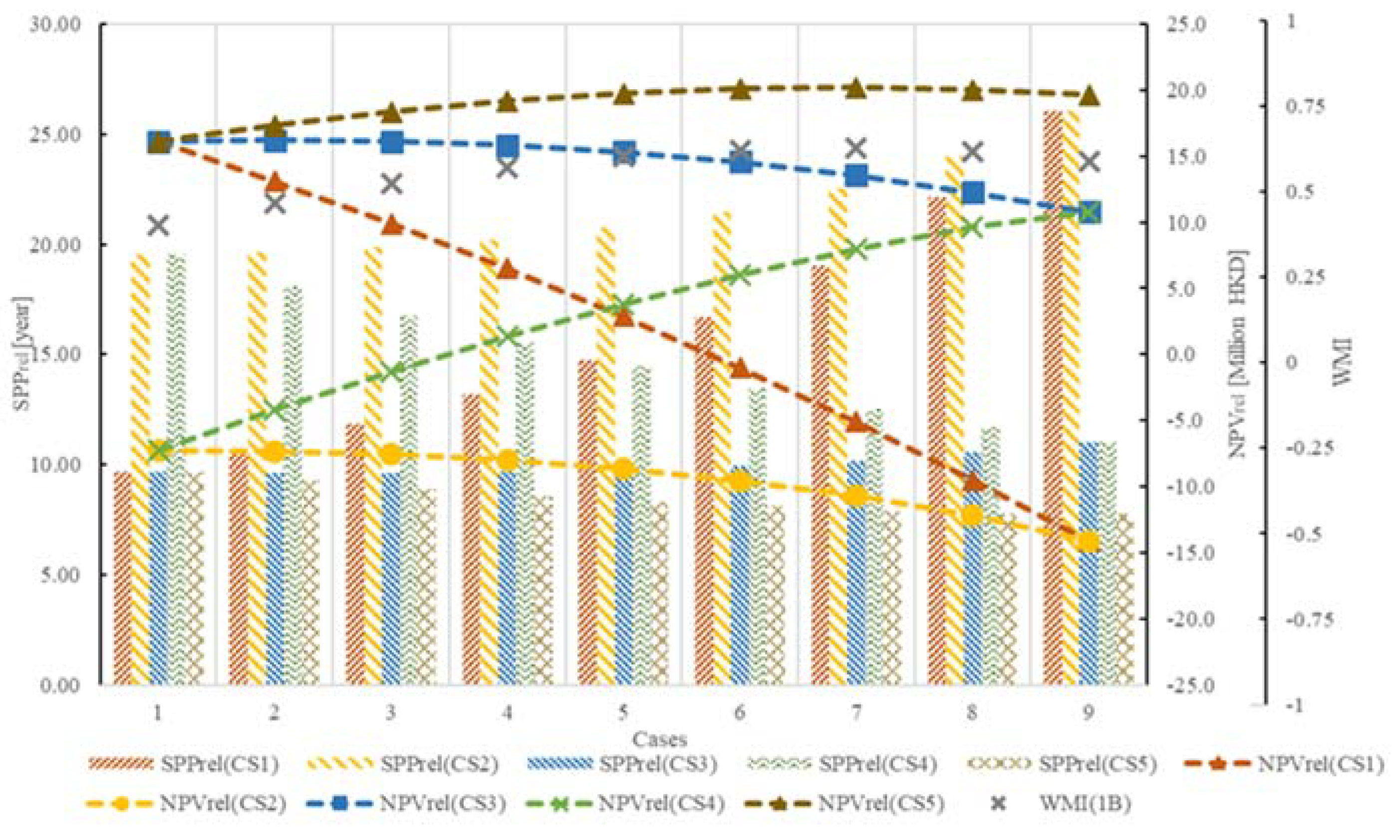
5.4.3. Economic Sensitivity Analysis for the Hybrid Zero-Emission System (Investigation of Single E-Boat)

Based on the study in Section 5.4.1, the best economic case is Case 1, which only applies FPV in the system. This result is based on the cost scenario (CS) in which WEC (45,630 HKD/kW) has a significantly higher capital cost than FPV (26,520 HKD/kW). In this CS, FPV is much cheaper than WEC, leading to the economic efficiency being highest when the integrated ocean energy systems are equipped with FPV only. In order to discuss more cost combinations and perform an economic sensitivity analysis, as shown in

Table 22. The capital cost scenarios of the Wave-FPV hybrid system.

Selected Group: G3.0 (1 Boat)	WEC (HKD/kW)	FPV (HKD/kW)	Boat PV (HKD/kW)	Boat Battery (HKD/kWh)
Capital Cost Scenario 1	45,630	26,520	37,331	1560
Capital Cost Scenario 2	45,630	46,800
Capital Cost Scenario 3	28,439	26,520
Capital Cost Scenario 4	28,439	46,800
Capital Cost Scenario 5	21,840	26,520

, in this section we will discuss five CS for the integrated ocean energy systems. The capital cost scenarios were developed on the basis of [57,58]. The last cost scenario has an assumed cost for WEC in order to project the desired outcome.

Instead of investigating Group 2.0, the selected analysis group is Group 3.0, which has one boat participating in the interaction with the boat-to-building function. The cruise velocity and distance are 15 km/h and 7.5 km. Case 1 is the pure FPV case with 5524.5 m² FPV. Then each case applies five units of WEC. Case 8 is the pure WEC case with 40 units of WEC. The total numbers of WECs for Case 2 to Case 8 are 5, 10, 15, 20, 25, 30 and 35 units, respectively. The areas of FPV are 4823.7, 4124.6, 3425.4, 2726.3, 2027.2, 1326.4, and 627.3 m², respectively.

As mentioned previously, CS1 has a higher capital cost for the WEC and a lower cost for the FPV. In Figure 20, for CS1 (red dashed line and bar), thanks to the lower cost of the FPV, the most beneficial case is Case 1, which has the shortest “SPP_rel” (9.66 years) and the highest “NPV_rel” (HKD 16.14 million), respectively. Correspondingly, in CS4 (green dash line and bar), the capital cost of the WEC is much lower than that of the FPV; in Case 9, 40 units of WEC are equipped, so the economic advantage of this case is the most obvious, with “NPV_rel” and “SPP_rel” of HKD 10.8 million and 11.02 years, respectively. All the combination cases in CS2 found it difficult to achieve any profit in either “SPPrel” or “NPVrel” due to the expensive capacity cost of the WEC and FPV. Of interest are another two cost scenarios. In the cost scenario CS3, since WEC and FPV are comparable in cost, there is no longer a lopsided economic advantage. In CS3, the greatest economic advantages occur in Cases 2 and 3, which are hybrid cases. This indicates that the decrease in the cost of WEC will benefit hybrid systems. Therefore, CS5 shows the predicted results. Once the capital cost of WEC drops to around 21,840 HKD/kW, the best economic case matches the best technical case.

5.5. Environmental and Economic Analysis, Limitations of the Current Study

5.5.1. Environmental and Economic Analysis

The simulation results were presented in Section 5.2.1 and Section 5.3.2, which discusses nine combinations of the two ORE systems. All investigated groups have a default cruising velocity of around 10 km/h and a cruising distance of 7.5 km. As shown in Figure 21a, the “CE_a” remains around 5.6 kg CO_2,eq/m².a from Case 1 to Case 8 without the involvement of any E-boats in the interaction, since the total design power generation is the same for these combinations. In particular, Case 9 has the minimum annual CO₂ emissions, considering that in this case, 40 units of WEC could generate more energy than in the other cases. Once E-boats are involved in the interaction (with only the building-to-boat function), the single boat provides an increase of 0.36 kg CO_2,eq/m² per year. The blue bar shows Group 3.1, which activates the boat-to-building function; those cases with more WEC applications could reduce the annual CO₂ emissions by around 0.1 to 0.2 CO_2,eq/m² per year.

The economic results were discussed in the previous sections, and although the lowest “CEa” combination was Case 9, with 40 WECs, this case would not be economically viable for 20 years. Based on the current market cost of renewable energy systems, a better option would be to apply Case 5 to keep profits positive.

Figure 21b compares the eight boats in Group 2.1 and Group 3.1 without or activating the boat-to-building function. The total annual “CE_a” of Group 2.1 indicates that each boat would increase by 0.36 kg CO_2,eq/m² per year, resulting in the “CEa” from Case 1 to Case 8 growing to 8.5 CO_2,eq/m².a. Case 9 goes to 7.0 CO_2,eq/m².a. After activating the boat-to-building function, Case 1 to Case 3 have more extensive areas of application of FPV. Therefore, these three cases lose the benefit of reduced carbon emissions. Considering the energy mismatch problem in Case 1 to Case 3, it would be more dependent on the grid charge for the building and boats. From Case 4 to Case 9, the advantages from the boat-to-building function are more obvious. A reduction of around 0.12 to 0.25 CO_2,eq/m² could be achieved in these six cases. Moreover, the increase of the number of boats will not result in greater economic returns. However, activating the boat-to-building function could significantly improve the relative NPV.

5.5.2. Limitations of the Current Study

In this study, the main indicator concerns for the environmental performance and climate effects were the annual operational equivalent CO₂ emissions of the hybrid system, “${\mathrm{CE}}_{\mathrm{a}}$”. This indicator only considers the emissions from the annual net direct energy. In other words, this study is focused on operational emissions instead of the total life cycle emissions. Moreover, the embodied emissions of floating photovoltaics, wave energy converters, and batteries of the boat are not considered. This limits the impact of the hybrid ocean renewable energy systems mentioned in this study on the climate.

In terms of economic factors, all of the comparisons of simple payback period and net present value are relative. There is a reference case as a benchmark to simplify the costing and focus on the economic analysis of the entire hybrid system. All the systems in the study were simply assumed to have 20 years of lifetime. Battery replacement was defined with a number of charging and discharging cycles above 2000 being the primary end-of-life point. Therefore, in the current study, the salvage value of the floating photovoltaics, wave energy converters, and batteries of the boat were also not considered. The consideration of the end-of-life management with respect to both emissions and economic aspects will be more comprehensive and environmentally friendly. These topics are beyond the research scope of the current study. Further study should be conducted on these topics.

In addition, the installation of ocean renewable energy systems on a large scale may cause adverse effects on the ecosystem. These disadvantages for the ocean and eco-environment should be better investigated when developing ocean energy generation systems in the future.

6. Conclusions

Although on-site renewable energy generation systems could help cover most of the energy demand of the building, on-site renewables are not stable, because different on-site renewable energy generators have different uncertainties and randomness due to the location and weather. This results in a mismatch between on-site generated renewable energy and building demand, considering the surplus renewable energy will be sent back to the grid. This study investigated a zero-energy hotel building supported by a hybrid ocean energy system that interacts with many zero-emission electric boats. Nine different combinations of floating photovoltaic and wave energy converters were investigated to compensate for the different fluctuations and uncertainties of the energy generated by the two different ocean energy systems. The impact of introducing the interaction between the electric boat and the building on the techno-economic performance of such hybrid systems was also discussed. Based on the simulation and analysis results, the key conclusions are summarized below.

Firstly, nine combinations of the hybrid ORE systems were designed to realize the zero-energy hotel building and cover the total annual electricity demand of the hotel building, approximately 230.27 kWh/m².a. Based on the same annual generation scenario when no electric boat is applied to the hybrid system, with 30 units of the wave energy converter and 1326.4 m² of floating photovoltaic (Case 7), this combination was able to reach the highest matching (WMI is 0.598) between the Wave-FPV generator and the building energy consumption. This also indicates that the total annual energy generation ratios of the WEC and FPV were 76% and 24%, respectively. The annual exported REe (86.85 kWh/m².a) and imported grid electricity (98.36 kWh/m².a) in this case were also the lowest among the nine cases. The annual net direct energy (“E_direct,a”) in this case was 11.51 kWh/m².a. After considering the interaction of one electric boat with the only building to boat function, although the WMI improvement was not significant (only around 0.9 to 1.8%), it can be seen that the “E_imp,a” and “E_exp,a” both decreased because of the interaction with only one E-boat, decreasing by 0.2% and 0.9%, respectively. The annual local renewable energy ratio in the electric boat integrated system (“${\mathsf{\eta }}_{\mathrm{EB},\mathrm{RE}}$”) in Case 7 was around 95.9%.

Secondly, more simulation groups were performed to investigate the effect of different cruising speeds and cruising distances on the interaction of the hybrid system with electric boats. The simulation results indicate that the faster the boat travels, the better the WMI is for the same cruising distance. Case 7 of Group 2.0 reached a WMI of 0.606 with a maximum cruising speed of 15 km/h. Moreover, the farther the boat travels, the better the WMI is when the boat travels at the same speed. The WMI of Group 2.6 Case 7 improved to 0.640 when the maximum cruising distance was 12.5 km. The reason for this is that because the boat only has the building to boat function, either accelerating or extending the sailing distance, the boat’s energy consumption increases. Therefore, the boat consumes more on-site residual renewable energy, improving the WMI.

Thirdly, based on the ORE combination in Case 7, more boats participate in the hybrid system, and all of them can activate the boat-to-building function. This indicates that as the number of mobile power sources increases, the total energy consumption of the boat increases. As expected, activating the boat-to-building function could increase the overall WMI by about 2–3%. The WMI can be increased by 0.2–0.5% for each additional boat, and the WMI growth rate decreases with the number of boats. However, a maximum WMI of 0.703 was obtained when 16 boats participated in the hybrid system, which occurs in Group 3.0, sailing at 15 km/h. This group has more time to interact with the building while maintaining the same sailing distance of 7.5 km. However, at the same time, due to the increase in the number of boats to 16, the negative impacts include a rather low “${\mathsf{\eta }}_{\mathrm{EB},\mathrm{RE}}$” (0.664), a rather high “E_direct” (38.71 kWh/m².a) and “CE_a” (18.82 kg CO_2,eq/m².a).

Fourthly, since the capital cost of FPV is much lower than that of WEC under the existing market cost scenario, the shortest simple payback period (9.59 years) and the second-highest relative “NPV_rel” (16.04 million HKD) were found when the hybrid systems were only equipped with FPV without the participation of electric boats. Based on the current market cost, it can be seen that when the number of WEC exceeds 20 units, it is difficult to achieve a positive value of NPV. Although the hybrid system Case 5 did not have the best technical performance and economic return, it could still be profitable over a 20-year life cycle. The hybrid system will continue the techno-economic analysis of boat and building interaction at different travel velocities and distances based on Case 5. In conclusion, Group 3.0 (with one boat, 20 units of WEC, and 2726.3 m² of FPV) had the shortest “SPP_rel” (14.77 years) and the best “NPV_rel” (HKD 2.86 million). After increasing the number of boats, because of the need to consider the cost of more boat batteries and PV, the best technical performance (WMI is 0.683) was found for Group 3.0 with 16 boats, with “SPP_rel” and “NPV_rel” of 15.45 years and HKD 1.67 million, respectively. However, the number of 16 boats was investigated as an extreme case. According to the designed profile of the hotel, the maximum number of E-boats is suggested to be eight. Therefore, for this study, when Group 3.0 had eight boats, the non-dominated WMI was 0.654, and the “SPP_rel” and “NPV_rel” were 15.63 years and HKD 1.61 million, respectively.

Lastly, five capital cost scenarios were proposed to investigate the cost sensitivity of the two ocean renewable energy sources in the hybrid system. It was found that if the capital cost of WEC continues to drop in the future, hybrid ORE systems will have better economic efficiency, which coincides with the best technical performance case as well. When the capital cost of FPV is higher than WEC, or the capital cost of WEC is higher than FPV, there will be higher economic efficiency returns when only fully implementing the cheaper renewable energy system.

References

1. IEA. 2019 Global Status Report for Buildings and Construction; United Nations Environment Programme: Nairobi, Kenya, 2019. [Google Scholar]
2. EMDS. Hong Kong Energy End-Use Data 2020; Electrical and Mechanical Services Department: Hong Kong, China, 2020. [Google Scholar]
3. Environment Bureau. Hong Kong’s Climate Action Plan 2030+. Environmental Bureau; The Government of the Hong Kong Special Administrative Region: Hong Kong, China, 2017. [Google Scholar]
4. United Nations. The Paris Agreement; United Nations: Brussels, Belgium, 2015. [Google Scholar]
5. European Commission. Nearly Zero-Energy Buildings; European Commission: Brussels, Belgium, 2014. [Google Scholar]
6. Wang, L.; Gwilliam, J.; Jones, P. Case study of zero energy house design in UK. Energy Build. 2009, 41, 1215–1222. [Google Scholar] [CrossRef]
7. Attia, S.; Gratia, E.; De Herde, A.; Hensen, J. Simulation-based decision support tool for early stages of zero-energy building design. Energy Build. 2012, 49, 2–15. [Google Scholar] [CrossRef] [Green Version]
8. Sobhani, H.; Shahmoradi, F.; Sajadi, B. Optimization of the renewable energy system for nearly zero energy buildings: A future-oriented approach. Energ Convers. Manag. 2020, 224, 113370. [Google Scholar] [CrossRef]
9. Cao, X.; Dai, X.; Liu, J. Building energy-consumption status worldwide and the state-of-the-art technologies for zero-energy buildings during the past decade. Energy Build. 2016, 128, 198–213. [Google Scholar] [CrossRef]
10. Arabkoohsar, A.; Behzadi, A.; Alsagri, A.S. Techno-economic analysis and multi-objective optimization of a novel solar-based building energy system; An effort to reach the true meaning of zero-energy buildings. Energy Convers. Manag. 2021, 232, 113858. [Google Scholar] [CrossRef]
11. Kaewunruen, S.; Sresakoolchai, J.; Kerinnonta, L. Potential Reconstruction Design of an Existing Townhouse in Washington DC for Approaching Net Zero Energy Building Goal. Sustainability 2019, 11, 6631. [Google Scholar] [CrossRef] [Green Version]
12. Gholami, H.; Røstvik, N.H.; Steemers, K. The Contribution of Building-Integrated Photovoltaics (BIPV) to the Concept of Nearly Zero-Energy Cities in Europe: Potential and Challenges Ahead. Energies 2021, 14, 6015. [Google Scholar] [CrossRef]
13. Tournaki, S.M.F.; Tsoutsos, R.; Morell, I.; Guerrero, Z.; Urosevic, A.; Derjanecz, C.; Nunez, C.; Rata, M.; Biscan, S.; Pouffary, S.; et al. Towards Nearly Zero Energy Hotels Technical Analysis and Recommendations. In Proceedings of the 5th International Conference on Renewable Energy Sources and Energy Efficiency, Istanbul, Turkey, 21–23 October 2021. [Google Scholar]
14. Beccali, M.; Finocchiaro, P.; Ippolito, M.G.; Leone, G.; Panno, D.; Zizzo, G. Analysis of some renewable energy uses and demand side measures for hotels on small Mediterranean islands: A case study. Energy 2018, 157, 106–114. [Google Scholar] [CrossRef]
15. Filipe, O.; Cunha, A.C.O. Benchmarking for realistic nZEB hotel buildings. Build. Eng. 2020, 30, 101298. [Google Scholar]
16. Nocera, F.; Giuffrida, S.; Trovato, M.R.; Gagliano, A. Energy and New Economic Approach for Nearly Zero Energy Hotels. Entropy 2019, 21, 639. [Google Scholar] [CrossRef] [Green Version]
17. Kahn Ribeiro, S.; Kobayashi, S.M.; Beuthe, J.; Gasca, D.; Greene, D.S.; Lee, Y.; Muromachi, P.J.; Newton, S.; Plotkin, D.; Sperling, R.; et al. Transport and Its Infrastructure. In Climate Change 2007, Mitigation; IPCC: Cambridge, UK; New York, NY, USA, 2007. [Google Scholar]
18. European Commission. A European Strategy for Low-Emission Mobility; European Commission: Brussels, Belgium, 2014. [Google Scholar]
19. Hafez, O.; Bhattacharya, K. Optimal design of electric vehicle charging stations considering various energy resources. Renew. Energy 2017, 107, 576–589. [Google Scholar] [CrossRef]
20. Sun, B. A multi-objective optimization model for fast electric vehicle charging stations with wind, PV power and energy storage. J. Clean. Prod. 2021, 288, 125564. [Google Scholar] [CrossRef]
21. Kumar, G.M.S.; Cao, S. State-of-the-Art Review of Positive Energy Building and Community Systems. Energies 2021, 14, 5046. [Google Scholar] [CrossRef]
22. Golla, N.K.; Sudabattula, S.K. Impact of Plug-in electric vehicles on grid integration with distributed energy resources: A comprehensive review on methodology of power interaction and scheduling. Mater. Today Proc. 2021, in press. [Google Scholar] [CrossRef]
23. Buonomano, A. Building to Vehicle to Building concept: A comprehensive parametric and sensitivity analysis for decision making aims. Appl. Energy 2020, 261, 114077. [Google Scholar] [CrossRef]
24. Chen, J.; Zhang, Y.; Li, X.; Sun, B.; Liao, Q.; Tao, Y.; Wang, Z. Strategic integration of vehicle-to-home system with home distributed photovoltaic power generation in Shanghai. Appl. Energy 2020, 263, 114603. [Google Scholar] [CrossRef]
25. Cao, S. The impact of electric vehicles and mobile boundary expansions on the realization of zero-emission office buildings. Appl. Energy 2019, 251, 113347. [Google Scholar] [CrossRef]
26. YC Synergy powers electric yachts with fuel cell technology. Fuel Cells Bull. 2014, 2014, 4. [CrossRef]
27. Al-Falahi, M.D.A.; Nimma, K.S.; Jayasinghe, S.D.G.; Enshaei, H.; Guerrero, J.M. Power management optimization of hybrid power systems in electric ferries. Energy Convers. Manag. 2018, 172, 50–66. [Google Scholar] [CrossRef] [Green Version]
28. Kim, Y.-R.; Kim, J.-M.; Jung, J.-J.; Kim, S.-Y.; Choi, J.-H.; Lee, H.-G. Comprehensive Design of DC Shipboard Power Systems for Pure Electric Propulsion Ship Based on Battery Energy Storage System. Energies 2021, 14, 5264. [Google Scholar] [CrossRef]
29. Tercan, S.H.; Eid, B.; Heidenreich, M.; Kogler, K.; Akyurek, O. Financial and Technical Analyses of Solar Boats as A Means of Sustainable Transportation. Sustain. Prod. Consump. 2021, 25, 404–412. [Google Scholar] [CrossRef]
30. Quirapas, M.A.J.R.; Taeihagh, A. Ocean renewable energy development in Southeast Asia: Opportunities, risks and unintended consequences. Renew. Sustain. Energy Rev. 2021, 137, 110403. [Google Scholar] [CrossRef]
31. Boh, S. World’s Largest Floating Solar Photovoltaic Cell Test-Bed Launched in Singapore. The Straits Times. 2016. Available online: https://www.straitstimes.com/singapore/worlds-largest-floating-solar-photovoltaic-cell-test-bed-launched-in-singapore (accessed on 10 December 2021).
32. Group, N. NYK to Participate in Demonstration of Tidal Energy in Singapore; NYK: Tokyo, Japan, 2018. [Google Scholar]
33. Offshore Energy. Philippines Gives Blessing to Utility Scale Tidal Energy Project. Available online: https://www.offshore-energy.biz/philippines-gives-blessing-to-utility-scale-tidal-energy-project/ (accessed on 10 December 2021).
34. Lavidas, G. Developments of energy in EU-unlocking the wave energy potential. Int. J. Sustain. Energy 2019, 38, 208–226. [Google Scholar] [CrossRef]
35. Hemer, M.A.; Manasseh, R.; McInnes, K.L.; Penesis, I.; Pitman, T. Perspectives on a way forward for ocean renewable energy in Australia. Renew. Energy 2018, 127, 733–745. [Google Scholar] [CrossRef]
36. Jiang, B.; Li, X.; Chen, S.; Xiong, Q.; Chen, B.-f.; Parker, R.G.; Zuo, L. Performance analysis and tank test validation of a hybrid ocean wave-current energy converter with a single power takeoff. Energy Convers. Manag. 2020, 224, 113268. [Google Scholar] [CrossRef]
37. Weiss, C.V.C.; Guanche, R.; Ondiviela, B.; Castellanos, O.F.; Juanes, J. Marine renewable energy potential: A global perspective for offshore wind and wave exploitation. Energy Convers. Manag. 2018, 177, 43–54. [Google Scholar] [CrossRef]
38. Cao, S. Comparison of the energy and environmental impact by integrating a H2 vehicle and an electric vehicle into a zero-energy building. Energy Convers. Manag. 2016, 123, 153–173. [Google Scholar] [CrossRef]
39. TRNSYS 18. Available online: http://sel.me.wisc.edu/trnsys/features/features.html (accessed on 10 December 2021).
40. Peel, M.C.; Finlayson, B.L.; McMahon, T.A. Updated world map of the Köppen-Geiger climate classification. Hydrol. Earth Syst. Sci. 2007, 11, 1633–1644. [Google Scholar] [CrossRef] [Green Version]
41. The University of Wisconsin-Madison. Solar Energy Laboratory of the University of Wisconsin-Madison, T.E.G., CSTB–Centre Scientifique et Technique du Bâtiment, TESS–Thermal Energy Systems Specialists, Section 8.7 Meteonorm Data. 2017. Volume 8. Available online: https://sel.me.wisc.edu/trnsys/features/trnsys18_0_updates.pdf (accessed on 15 October 2021).
42. Meteotest, A.G. Meteonorm. Available online: https://meteonorm.com/en/ (accessed on 10 December 2021).
43. E.M.S.D. Performance-Based Building Energy Code; The Government of the Hong Kong Special Administrative Region: Hong Kong, China, 2007. [Google Scholar]
44. SOELCAT 12. Available online: https://soelyachts.com/soelcat-12/ (accessed on 10 December 2021).
45. 340W NeON®. 2 Black Solar Panel for Home. Available online: https://www.lg.com/us/business/solar-panels/lg-lg340n1k-l5 (accessed on 10 December 2021).
46. The University of Wisconsin-Madison. Multizone Building Modeling with Type56 and TRNBuild of the TRNSYS Document Package. Solar Energy Laboratory of the University of Wisconsin-Madison, T.E.G., CSTB–Centre Scientifique et Technique du Bâtiment, TESS–Thermal Energy Systems Specialists. 2017. Volume 5. Available online: https://sel.me.wisc.edu/trnsys/ (accessed on 15 October 2021).
47. LLC of Madison. Type 567: Glazed Building-Integrated PV System (Interacts w/Type 56); Section 3.6; TESS–Thermal Energy Systems Specialists; LLC of Madison: Madison, WI, USA, 2013; Volume 3. [Google Scholar]
48. FuturaSun. Available online: https://www.futurasun.com/en/ (accessed on 10 December 2021).
49. Wave Dragon. Available online: http://www.wavedragon.net/ (accessed on 10 December 2021).
50. Hald, T.; Frigaard, P. Forces and Overtopping on 2. Generation Wave Dragon for Nissum Bredning; Hydraulics & Coastal Engineering Laboratory, Department of Civil Engineering, Aalborg University: Aalborg, Denmark, 2001. [Google Scholar]
51. Giovanna Bevilacqua, B.Z. Overtopping Wave Energy Converters: General Aspects and Stage of Development. 2011. Available online: http://amsacta.unibo.it/3062/1/overtopping_devicex.pdf (accessed on 10 December 2021).
52. Parmeggiani, S.; Chozas, J.F.; Pecher, A.; Friis-Madsen, E.; Sørensen, H.C.; Kofoed, J.P. Performance Assessment of the Wave Dragon Wave Energy Converter Based on the EquiMar Methodology. In Proceedings of the 9th European Wave and Tidal Conference, Southampton, UK, 5–9 September 2011. [Google Scholar]
53. Cao, S.; Hasan, A.; Sirén, K. On-site energy matching indices for buildings with energy conversion, storage and hybrid grid connections. Energy Build. 2013, 64, 423–438. [Google Scholar] [CrossRef]
54. Cao, S.; Mohamed, A.; Hasan, A.; Sirén, K. Energy matching analysis of on-site micro-cogeneration for a single-family house with thermal and electrical tracking strategies. Energy Build. 2014, 68, 351–363. [Google Scholar] [CrossRef]
55. Bank, T.W. Real Interest Rate (%)-Hong Kong SAR, China. Available online: https://data.worldbank.org/indicator/FR.INR.RINR?end=2019&locations=HK&start=2010&view=chart (accessed on 10 December 2021).
56. CLP. CLP Sustainability Report 2020; CLP: Hong Kong, China, 2020. [Google Scholar]
57. Wave Dragon 1.5 MW. Available online: https://energiforskning.dk/sites/energiforskning.dk/files/slutrapporter/wd15mwv4_efm-17.pdf (accessed on 10 December 2021).
58. Martins, B.P. Techno-Economic Evaluation of a Floating PV System for a Wastewater Treatment Facility; KTH School of Industrial Engineering and Management Energy Technology: Stockholm, Sweden, 2019. [Google Scholar]
59. NREL. Distributed Generation Energy Technology Capital Costs. Available online: https://www.nrel.gov/analysis/tech-cost-dg.html (accessed on 10 December 2021).
60. Hsieh, I.Y.L.; Pan, M.S.; Chiang, Y.-M.; Green, W.H. Learning only buys you so much: Practical limits on battery price reduction. Appl. Energy 2019, 239, 218–224. [Google Scholar] [CrossRef]
61. CLP. Tariff and Charges. Available online: https://www.clp.com.hk/en/customer-service/tariff (accessed on 10 December 2021).
62. CLP. Renewable Energy Feed-in Tariff. Available online: https://www.clp.com.hk/en/community-and-environment/renewable-schemes/feed-in-tariff (accessed on 10 December 2021).
63. Official Exchange Rate (LCU per US$, Period Average)-Hong Kong SAR, China. Available online: https://data.worldbank.org/indicator/PA.NUS.FCRF?end=2019&locations=HK&start=2011 (accessed on 10 December 2021).
64. Fanger, P.O. Thermal Comfort. Analysis and Applications in Environmental Engineering; Danish Technical Press: Copenhagen, Denmark, 1970. [Google Scholar]
Figure 1. Schematic of a coastal hotel building supported by the Wave-FPV hybrid renewable energy generation system interacting with a zero-emission electric boat. (“REe Surplus_1st” is the renewable energy remaining after covering the building’s demand, “REe Surplus_2nd” is the renewable energy remaining after charging the E-boat, “Short_1st” is the energy shortage of the building supported by the E-boat, “Short_2nd” is the energy shortage of the building supported by the grid).
Energies 14 08465 g001
Figure 2. The monthly dry and wet bulb temperature, seawater temperature and total solar radiation.
Energies 14 08465 g002
Figure 3. The monthly significant wave height.
Energies 14 08465 g003
Figure 4. The location of the research project is on Cheng Chau Island, Hong Kong (FPV refers to floating photovoltaics, WEC denotes wave energy converters).
Energies 14 08465 g004
Figure 5. The duration curves of the heating, cooling and electric demands of the hotel building.
Energies 14 08465 g005
Figure 6. The designed E-boat tourist schedule and night charge schedule.
Energies 14 08465 g006
Figure 7. E-boat velocities, maximum running hours and corresponding energy consumptions.
Energies 14 08465 g007
Figure 8. The flow chart of the research steps, methodology, and assessment criteria.
Energies 14 08465 g008
Figure 9. The comparison of different renewable energy generation combination cases and corresponding matching capabilities without and with electric boat participation. (“pGen_FPV” is the energy generated from floating photovoltaics, “pGen_Wave” is the energy generated from wave energy converters, “WMI” is the weighted matching index, “ŋEB,RE” is the annual local renewable energy ratio in the electric boat integrated system).
Energies 14 08465 g009
Figure 10. The comparison of different renewable energy generation combination cases and their corresponding matching capabilities without and with electric boat participation.
Energies 14 08465 g010
Figure 11. The monthly energy demand, generation, and matching capability.
Energies 14 08465 g011
Figure 12. The hourly energy demand, generation, and matching capability on 10 February (daily total energy demand is 0.48 kWh/m2, energy generation is 0.27 kWh/m2, daily average WMI is 0.64).
Energies 14 08465 g012
Figure 13. The hourly energy demand, generation, and matching capability on 10 June (daily total energy demand is 0.65 kWh/m2, energy generation is 0.60 kWh/m2, daily average WMI is 0.74).
Energies 14 08465 g013
Figure 14. The comparison of the annual net direct energy consumption, “Edirect,a”, the annual local renewable energy ratio in the electric boat integrated system, “ŋEB,RE”, and the matching capability among the different cruise velocity groups.
Energies 14 08465 g014
Figure 15. The comparison of the annual net direct energy consumption, “Edirect,a”, the annual local renewable energy ratio in the electric boat integrated system, “ŋEB,RE”, and the matching capability among different cruise distance groups.
Energies 14 08465 g015
Figure 16. The comparison of the annual net direct energy consumption, “Edirect,a”, the annual local renewable energy ratio in the electric boats integrated system, “ŋEB,RE”, and the matching capability among the different cruise velocity groups. (a) Without the boat-to-building function. (b) With the boat-to-building function.
Energies 14 08465 g016aEnergies 14 08465 g016b
Figure 17. The comparison of the annual net direct energy consumption “Edirect,a”, the annual local renewable energy ratio in the electric boats integrated system “ŋEB,RE”, and the matching capability among the different cruise distance groups. (a) Without the boat-to-building function. (b) With the boat-to-building function.
Energies 14 08465 g017
Figure 18. The comparison of different renewable energy generation combination cases and corresponding relative simple payback period (SPPrel), relative net present value (NPVrel), emissions, and matching capability without and with electric boat interaction.
Energies 14 08465 g018
Figure 19. The comparison of the annual CO2 emissions “CEa”, the relative simple payback period (SPPrel), relative net present value (NPVrel), and matching capability among different cruise velocity groups. (a) Without boat-to-building function. (b) With boat-to-building function.
Energies 14 08465 g019
Figure 20. The economic sensitivity analysis for the hybrid zero-emission system.
Energies 14 08465 g020
Figure 21. The environmental and economic analysis for the hybrid system. (a) Without and with single boat interaction. (b) With 8-boat interaction.
Energies 14 08465 g021aEnergies 14 08465 g021b