Article

Energy and Carbon Emission Efficiency Prediction: Applications in Future Transport Manufacturing

by
Ragosebo Kgaugelo Modise
*,
Khumbulani Mpofu
and
Olukorede Tijani Adenuga
Department of Industrial Engineering, Tshwane University of Technology, Pretoria 0001, South Africa
*
Author to whom correspondence should be addressed.
Energies 2021, 14(24), 8466; https://doi.org/10.3390/en14248466
Submission received: 26 September 2021 / Revised: 25 November 2021 / Accepted: 3 December 2021 / Published: 15 December 2021

Abstract

:
The long-term impact of high-energy consumption in the manufacturing sector results in adverse environmental effects. Energy consumption and carbon emission prediction in the production environment is an essential requirement to mitigate climate change. The aim of this paper is to evaluate, model, construct, and validate the electricity generated data errors of an automotive component manufacturing company in South Africa for prediction of future transport manufacturing energy consumption and carbon emissions. The energy consumption and carbon emission data of an automotive component manufacturing company were explored for decision making, using data from 2016 to 2018 for prediction of future transport manufacturing energy consumption. The result is an ARIMA model with regression-correlated error fittings in the generalized least squares estimation of future forecast values for five years. The result is validated with RSS, showing an improvement of 89.61% in AR and 99.1% in MA when combined and an RMSE value of 449.8932 at a confidence level of 95%. This paper proposes a model for efficient prediction of energy consumption and carbon emissions for better decision making and utilize appropriate precautions to improve eco-friendly operation.

1. Introduction

Transport manufacturing is one of the most important sectors in the industry, affecting economic growth and job creation, which impact energy consumption [1]. Due to climate change, the estimation, reduction and quantification of emitted gasses are essential in major manufacturing sectors [1]. The manufacturing sector is responsible for a large portion of energy consumption and represents a significant source of greenhouse gas (GHG) emissions. This paper focuses on the automotive sector due to its high contribution to the growth of the transport manufacturing industry and the economic growth of South Africa, accounting for 29.9% of the manufacturing output of South Africa in 2018 [2]. The automotive industry accounting for 6.4% of the gross domestic product (GDP) of South Africa in 2019—4% through manufacturing and 2.4% through the retail market [3,4]. Automotive component manufacturing transforms unprocessed materials into an end-user product. The process involves energy consumption and use of acerbic fluids, results in scrap, contributes to sound and particle pollution, etc., resulting in environmental contamination [5]. Government carbon tax regulations imposed on manufacturers put pressure on industry stakeholders to reduce their carbon footprint and energy demand, while decreasing their electricity supply. While energy efficiency is recognized globally as a critical solution to reducing energy consumption, the management of global carbon dioxide (CO2) emissions complements climate change policies, decreases the costs of reducing carbon emissions, and improves economic competitiveness. The adoption of modern, emerging technologies is thus critical for the present and the future [6].
Forecasting has become the cornerstone of decision making, including business decisions. Forecasting can assist companies in development and decision making [7]. Electricity/energy estimation made considering carbon emissions assist manufacturing companies in determining and improving their environmental management systems, because appropriate safety measures may be implemented in advance to achieve an eco-friendly society [8]. Predictions of energy consumption and carbon emissions using a time-series (TS) forecasting technique are vital to assisting a company’s energy improvement and carbon efficiency activities. Climate change targets to reduce CO2 emissions require continuous improvement in technologies, investment in innovative energy and resource efficiency, a reduction in GHG initiatives and involvement in climate science research.
In the past two decades, various TS forecasting techniques have been used to predict energy consumption in the manufacturing sector [9]. TS forecasting is a hot research topic in the domain of science and engineering. The primary objective of TS analysis is to develop a mathematical model that can forecast future observations on the basis of available data [10]. Khandelwal et al. [11] elaborated TS forecasting as the use of a model to predict future values based on previously observed values [12]. Popular time-series forecasting techniques mostly used for energy and carbon predictions include artificial neural networks (ANNs) [13,14,15,16], auto-regressive integrated moving average (ARIMA) [17] and support vector machines (SVMs) [18]. Kant and Sangwan [18] predicted the power consumed in machining processes using support vector regression (SVR) and ANN techniques, and the study results confirmed that ANN performs better in predictions. Saleh et al. [19] investigated CO2 emissions using an SVM prediction model, considering variable energy consumption to have an impact on the emergence of CO2 emissions. The authors identified how increased consumption of electrical power is intimately linked with increased CO2 emissions.
Further studies and reviews on forecasting energy consumption and GHG emissions using ARIMA for a pig iron manufacturing organization were conducted to determine the current and future trends of indicators for better environmental policy [20]. Shan et al. [21] proposed a model control method for charging and discharging thermal energy storage to achieve high efficiency. A lightweight Internet of Things framework for predicting energy use at a localized level used a hybrid model based on ARIMA (SVR) and particle swarm optimization (PSO) proposed by [22] to predict the energy use from supplied data. Hybrid research was introduced by [23], using an ARIMA, convolutional neural network (CNN), long–short-term memory network (LSTM) model to forecast the future price of carbon. The results confirmed that the ARIMA–CNN–LSTM model can achieve better prediction accuracy than benchmark models in terms of root mean square error (RMSE), mean absolute prediction accuracy and mean absolute percentage error (MAPE). Fan et al. [24] proposed a novel ARIMA–LSTM hybrid model that considered the advantages of linearity and non-linearity, in terms of impact on manual operations, and the hybrid yielded better results. The gap identified based on the reviewed literature of limited studies on prediction of energy and carbon emission efficiency for decision making is that increased consumption of electrical power is intimately linked with increased CO2 emissions. The development of an analytical tool for mitigating and lowering an organization’s carbon tax will assist in prediction of carbon emissions based on energy consumption, while the implementation of energy efficiency measures that prompted the adoption of ARIMA was largely due to its popularity in linear applications within manufacturing sectors. ARIMA models, pioneered by Box and Jenkins, are the most popular and effective statistical models for TS [25], based on the fundamental principle that the future values of a TS are generated from a linear function of the past observations’ terms [11]. The autoregressive (AR) character of TS models indicates that the present value of any variable is determined by its past value and some adjustment factors.
This paper presents an evaluation of the obtained data on electricity generated with carbon components, the development of a mathematical model with related construct, and the validation of residual errors on the TS data to predict the forecast error for correctional purposes using Pandas in Python for an automotive component manufacturing company in South Africa. The prediction of energy consumption and carbon emissions aimed at helping the automotive company to make better decisions, with precautions to improve eco-friendly operation. The next section provides an overview of a literature review on transport manufacturing, automotive component manufacturing, and the energy consumption and carbon emissions of the South African automotive industry in terms of trends in the application of TS in the prediction of energy consumption and carbon emissions efficiency. Section 3 presents the materials used in this study and the application of the ARIMA model. Section 4 gives the results of the developed TS model. Section 5 discusses the steps and implications, while Section 6 summarizes the inherent properties of TS with an increase or a decrease in seasonality trends as variations in the period prompted by loading TS in Python for this study.

2. Literature Review

2.1. Transport Manufacturing: Automotive Component Manufacture

The transport manufacturing industry is facing an ongoing challenge to improve its production processes and mitigate the carbon emissions produced. The significant increase in overall vehicle production is directly linked to an increase in energy costs and environmental impacts [26]. The global increase in vehicle users is causing genuine concerns around ecological degradation of the ozone layer, lower air quality, climatic change, exhaustion of oxygen and unfavorable effects on green environments [27]. A report by the European Commission has stressed that the transport sector is of utmost importance in terms of economic growth, and it is widely acknowledged that targeted innovations and research activities are key to fostering competitiveness in the future of the transport sector [28]. Research conducted in the United State highlights that transport manufacturing is the eighth largest industrial energy consumer, and energy expenditure has increased by 20%, along with electricity purchase by almost 10% [29]. Transportation ecosystem sustainability has become vital to reducing GHG emissions, with the need to combat fossil fuel dependence and air pollution. Electric vehicles (EVs) are a future solution to mitigate the harmful effects of GHG emissions from petroleum fuel vehicles, and product life cycle analysis is key to each engineering step of manufacturing processes. Investment in the smart manufacturing industry, driven by new technologies such as big data analytics, Internet of Things (IoT), cybersecurity and cloud computing, is a foreseeable solution to manage system complexity, improve production performance, increase information visibility and gain competitive advantages in the global market [30,31].

2.2. The South African Automotive Industry

The global trend in transportation industry transformation and the South African automotive revolution began in 1924, with the emergence of energy consumption and carbon emissions regulation (Figure 1). In 2011, the South African government held an automotive week in East London, with emphasis on achieving a green economy. As a developing country, to remain competitive and relevant, South African automotive manufacturers have to adjust to the green economy to survive the future trend.
In 2020, the broader automotive industry’s contribution to the gross domestic product (GDP) stood at 4.9% (2.8% in manufacturing and 2.1% in retail market), a downward trend from 6.4% in 2019 due to the severe impact of COVID-19 lockdown restrictions on the country [5]. As the largest manufacturing sector in the country’s economy, a substantial 18.7% value addition to the domestic manufacturing output was derived from vehicle and automotive component manufacturing activity, which continues to position the industry and its broader value chain as key players within South Africa’s landscape of industrialization. Automotive manufacturing consumes a substantial amount of resources and involves complex energy-intensive processes that result in carbon emissions. Process sustainability requires efforts towards the low carbon emissions in automotive manufacturing processes with increased productivity [26].

2.2.1. Trends in South African Automotive Industry Energy Consumption and Carbon Emissions

There are limited recent available data for the component manufacturing sector, but an obtained report confirms that there are 167 vehicle manufacturers and 292 vehicle component manufacturers in South Africa [32]. The National Cleaner Production Centre (NCPC) implemented energy management saving activities for up to 13 automotive companies, with projected savings of 75,534,000 kwh of electricity and financial costs savings of R41,543,700 ($2,957,858), and a reduction in estimated CO2 emissions by 72,362 tons [33].
Coal is the main source of energy in South Africa, with 75% of total energy consumption due to manufacturing activities, which results in high CO2 emissions [33,34]. The main significant electricity users (SEUs) are compressed air systems, idling machines, wet scrubbers, paint shops, ovens and driers, cooling compressors, chillers and lights. The concentration of CO2 in the atmosphere has been tracked since 1958, and burning fossil fuels has contributed to 67% of global CO2 emissions, with a significant contribution from South Africa [20]. Energy utilization contributes to 1.5% of global carbon emissions, with South Africa leading with extensive energy use [21]. South Africa ranked as the 14th largest emitter of GHGs [12], with a heavy reliance on the use of coal and little capacity to limit carbon emissions. It is the responsibility of companies to ensure that their emissions are minimized by implementing energy measures that have a direct positive impact on the electricity generated. Almost all industrial activities entail carbon emissions; for instance, transportation, material extraction, end-of-life management of used products, and production from earth crust activities [24].

2.2.2. Energy and Carbon Emission Efficiency in Automotive Manufacturing

Energy efficiency (EE) is an important energy resource initiative that can help to meet future energy savings and reduce costs, thereby achieving a reduction in carbon emissions in future transport manufacturing (FTM). EE is recognized globally as a critical solution to reducing energy consumption, managing global CO2 emissions and improving economic competitiveness [35]. Research studies in energy and carbon efficiency for transport manufacturing and electricity management solutions in the context of industry 4.0 integration and demand response [36] show that approximately 30% of global energy consumption is due to the transportation sector, which is becoming the focus area in the decarbonization of global energy utilization [37].
Several improvements to carbon emissions in vehicle manufacturing processes are required. Activities involving manufacturing of a car (press, body, paint and assembly shops) may consume up to 700 kwh/vehicle [38]. The following publications focused on the application of energy efficiency policies in different sectors [38,39,40,41,42], general trading and decision making [43,44], ICT [45], and the building sector [39]. Other energy efficiency related research includes industry application in the supply chain [46], the impact of the South African energy crisis on emissions [47], carbon accounting [48] and prediction of carbon emissions [49]. The manufacturing sector consumes a high amount of energy and emits more, and extensive research has been conducted on energy efficiency in manufacturing, focusing on improvement [50], low-cost energy efficiency measures [51] and energy management including energy efficiency [52]. Further studies have focused on energy efficiency in manufacturing systems and processes [53,54,55]. Researchers working on energy efficiency have taken great interest in modelling energy efficiency in manufacturing, including rail manufacturing [56,57,58] and carbon dioxide prediction [59]. Saleh et al. [19] presents a review of the related literature on carbon emissions in terms of general applications and accounting, while [60] reviews the literatures on the causal relationship between energy consumption, price and emissions with focus on the implications of improved emissions and integraion of energy efficiency and carbon emissions in the industry. [61,62]. The benefits of improved EE in transport manufacturing are substantial such as increased productivity, fewer rejected parts and waste, a reduction in emissions and lower expenditure and improvements that can be apply in all industries. Key opportunities for improvement in energy efficiency and carbon efficiency in future transport manufacturing requires the application of current fourth industrial revolution technologies and prediction of future trends in consumption within the value chain of transport manufacturing, as well as envisaged carbon emissions. This will assist in mitigation of unnecessary energy use and will result in reduced emissions.

2.2.3. Application of Time Series in the Prediction of Energy and Carbon Emission Efficiency

In the past two decades, various studies applied forecasting techniques using TS to predict energy consumption in the manufacturing sector [63]. The domain of engineering science is a very active research area in TS forecasting and future value prediction for decision making based on the previous data distribution, which requires a deep understanding of variance, mean, kurtosis and skewness [64]. The aim of using TS analysis is to develop a mathematical model based on the currently available data to forecast future observations. Time-series analysis are divided into two types: univariate and multivariate. Univariate uses single observed recorded data over time, for hourly energy consumption. Multivariate analysis uses a group of variables and interactions among the considered variables [54]. This study adopted the univariate TS technique due to the flexibility and linearity of the technique that has been widely used in the energy and carbon industry [8,20,23,65,66,67,68].
Hornik et al. [13] used ARIMA to forecast energy consumption and GHG emissions in India’s pig iron sector, and the results presented indicators for current and future trends to interested managers for better decision making on the environment. The results of this study confirm that both energy consumption and GHG emission are best-fitted models. Rehman et al. [10] projected the CO2 emissions sector in Pakistan using ARIMA and other methods until 2030, and gave suggestions for how policy makers can make better decisions; the results showed an increasing trend in CO2 emissions from the manufacturing, energy, and transport sectors in Pakistan, which will cause significant problems if the government fails to respond to this sector-related issue appropriately.

3. Materials and Methods

3.1. Secondary Data for This Study

In this section, the focus is on the material used to model the data on electricity generated for a tier two automotive company for prediction of future transport manufacturing energy consumption and carbon emissions. Secondary data obtained for this study were from the National Cleaner Production Centre through its energy management-training program from 2016 to 2018, as presented in Table 1. The carbon emission equivalent was derived using compared country-specific energy according to Intergovernmental Panel on Climate Change (IPCC) 2006 emission factors for coal mining. The inherent properties of TS with seasonality trends increase or decrease as variations in the period and prompted the authors to load TS in Python for this study. The code for statistical plotting was the moving average/variance of the previous year, while testing for stationarity with a non-stationary null hypothesis performed using Dickey–Fuller tests. We concluded with aggregation, smoothing and polynomial fitting of data to the regression model.
Figure 2 provides the process flow for TS prediction using Python programming with rolling statistics in Pandas. Based on the outlined data in Table 1, data were captured- on energy consumption as electricity generated and CO2 emissions; these make up the columns of the y axis, with the date as an index on the x axis.
The trend, seasonality, time variance and other non-linear properties in the observed data, as deduced through time plotting, help to determine the different possible order and logarithmic transformation for variance stabilization side by side sample plots of autocorrelation functions (ACFs) and partial autocorrelation functions (PACFs) [48]. Auto-regression specifies a regression of a variable against itself. The model forecasts the variable using a combination of past value linearity of the variable [47]. In the real world, where there is a lot of uncertainty and change occurring rapidly, energy consumption and carbon emissions vary due to uncertainty, with many random series experiencing periodic change. Adjusting these non-stationary periodic stochastic processes, according to periodic intervals, eliminates the periodicity effect on the forecasted results [30]. With the stationary models methodology, some adjustments were needed before modelling of non-stationary series. It was important to plot the data and analyze it visually, as shown in Figure 2, which gives a graphic representation of the data. Dickey and Fuller [47] stated that different trends and stationarity of the same TS imply different predictions and hence the “unit root test” was applied to determine use-forecasting models for different applications. The statistical procedure employed a unit root test to determine the stationarity commonly used for the test. Augmented Dickey–Fuller (ADF) tests investigate the stationarity and integration of the variables, and test the design based on the null hypothesis [50]. Estimation was applied to a selected model to determine the maximum likelihood in back-casting, as postulated by Box and Jenkins (1976). Diagnostic checking is the vital principle of ARIMA that describes stationary times, and it is imperative for the identification process to transform TS data to stationary values via pre-differencing transformation. Estimating and eliminating the trend are considered important transformations in reducing the trend in the case of a significant positive trend; transformations can be applied to penalize higher values more than smaller values. In this study, we applied log transformation, a moving average considered by the average of the past years, i.e., 12 values. The rolling mean of the past 11 values was not defined, but windows 12 defined the exponential decay. Differencing can eliminate (or reduce) a trend and seasonality [38]. To determine the stationary, we considered two methods in statistical procedures: the rolling average [49] and an augmented Dickey-Fuller (ADF) test [36]. Rolling averages are a chart analysis-type technique used to examine collected survey data over extended periods to smooth out data series [49]. Pretorius et al. [47] further elaborates the analysis of the model’s stability in a more visual technique.

3.2. Methods

Application of ARIMA Model

ARIMA models represent different types of TS. This assumes future values have linear correlation with current and past values, which, by approximation, is not adequate for non-linear problems [57]. ARIMA is a statistical base method for prediction using historical data [11] that gained popularity among researchers due to its vast applications in manufacturing [9]. The models are known for their notable forecasting accuracy and flexibility in different applications [60]. ARIMA models as a univariate is an expression of how variables respond with stochastic dissimilarity [11,13]. The popularity of these is due to the statistical properties proposed by Box and Jenkins in the 1970s [59], with a forecast value that is dependent on the lagged value of the previous values.
It is expressed mathematically as (p, d, q), with estimated appropriate values for p, d, and q as presented in Equations (1) and (2):
( B b d ) p   y W t ( 1 B b d ) d = δ + θ q ( B b d ) a t
p   1   B b d 2   B b d 2 p   B b d p  
θ q ( B b d ) = 1 θ 1 ( B b d ) θ 2 B 2 θ p B b d 2 p
In the expression, W t is the TS; B b d is the backward shift operator; d is the regular differences order; and at-1 are independent random shocks. The series is a white noise process, and ∅p ( B b d ) and θq ( B b d ) are polynomials in   B b d of order p and q, respectively. The roots of ∅p ( B b d ) = 0 and θq ( B b d ) = 0 should lie outside the unit circle.
Thus, the order of the model as p is written as follows:
W t = c + ϕ 2 W t 1 + ϕ 2 W t 2 + + ϕ 2 W t p + ε t
where ε t   is the white noise, a multiple regression with lagged predictor values, referred to as an AR (p) model. In this study, we used the moving average to forecast the past errors in the regression and the future values with the formula:
W t = c + ε t + θ 1 ε t 1 + θ 2 ε t 2 + + θ q ε t q
where is ε t white the noise. We refer to this as an MA (q) model, a moving average model of order q. Of course, we do not observe the values of ε t , so it is not a regression in the usual sense. W t can be thought as a weighted moving average of the past few forecast errors.

4. Results

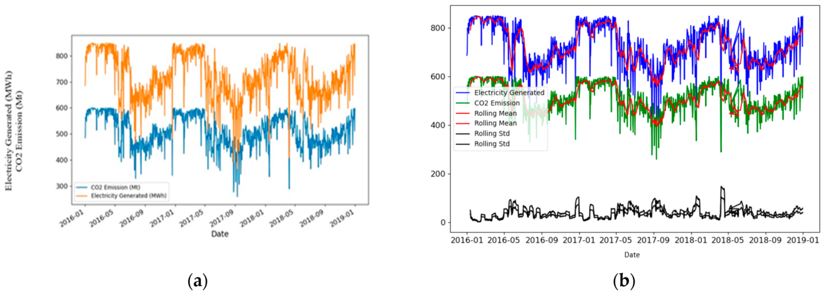
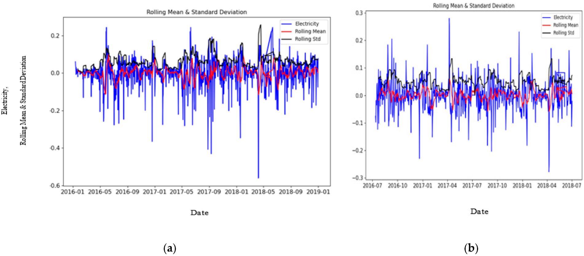
The model provides predictions for the calculation of RSS to determine the auto-regression model (p) using the differencing of the phrased dataset (d) to make the TS stationary in a supervised learning approach with dependency on the lagged residual error from the applied moving average model (q) in Figure 3, which is based on the original data collected for this study. Figure 4 presents a graphical representation of the pre- and post-estimation, eliminating trend and seasonality. This depicts the elimination of the residual electricity generated and CO2 data errors and seasonality components of the phrased dataset in terms of the rolling mean and standard deviation.
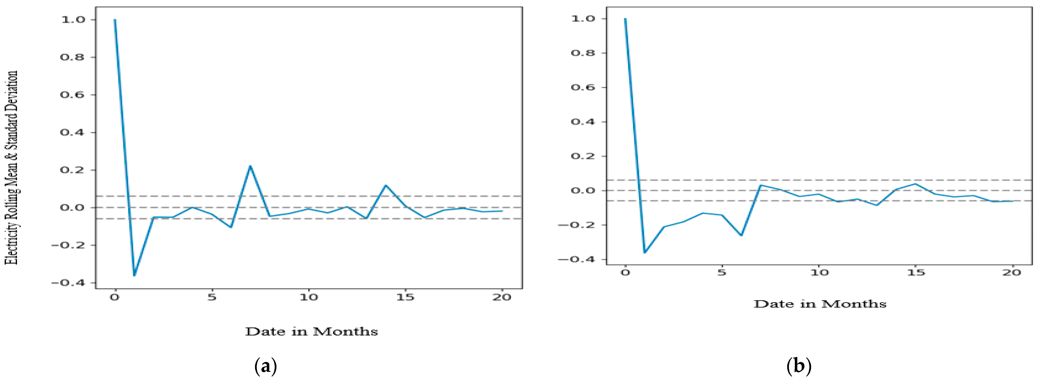
The adoption of the ARIMA model assumes there is an underlying process that motivates the raw observations in the residual errors of the forecasts from the model. Figure 5 provides a positive correlation with the first two to seven lags, which is significant to the first five lags as a good starting point for AR. The graphs represent ACFs and PACFs with two dotted lines, either side of the zero, showing the confidence intervals used to determine q = 0.5 and p = 0.5. The figure provides information on the autocorrelation cutoff and after the second lag, the value is estimated to be q, while the partial autocorrelation cuts off after two lags is estimated to be p based on the autocorrelation and partial correlation patterns denoted in Table 2.
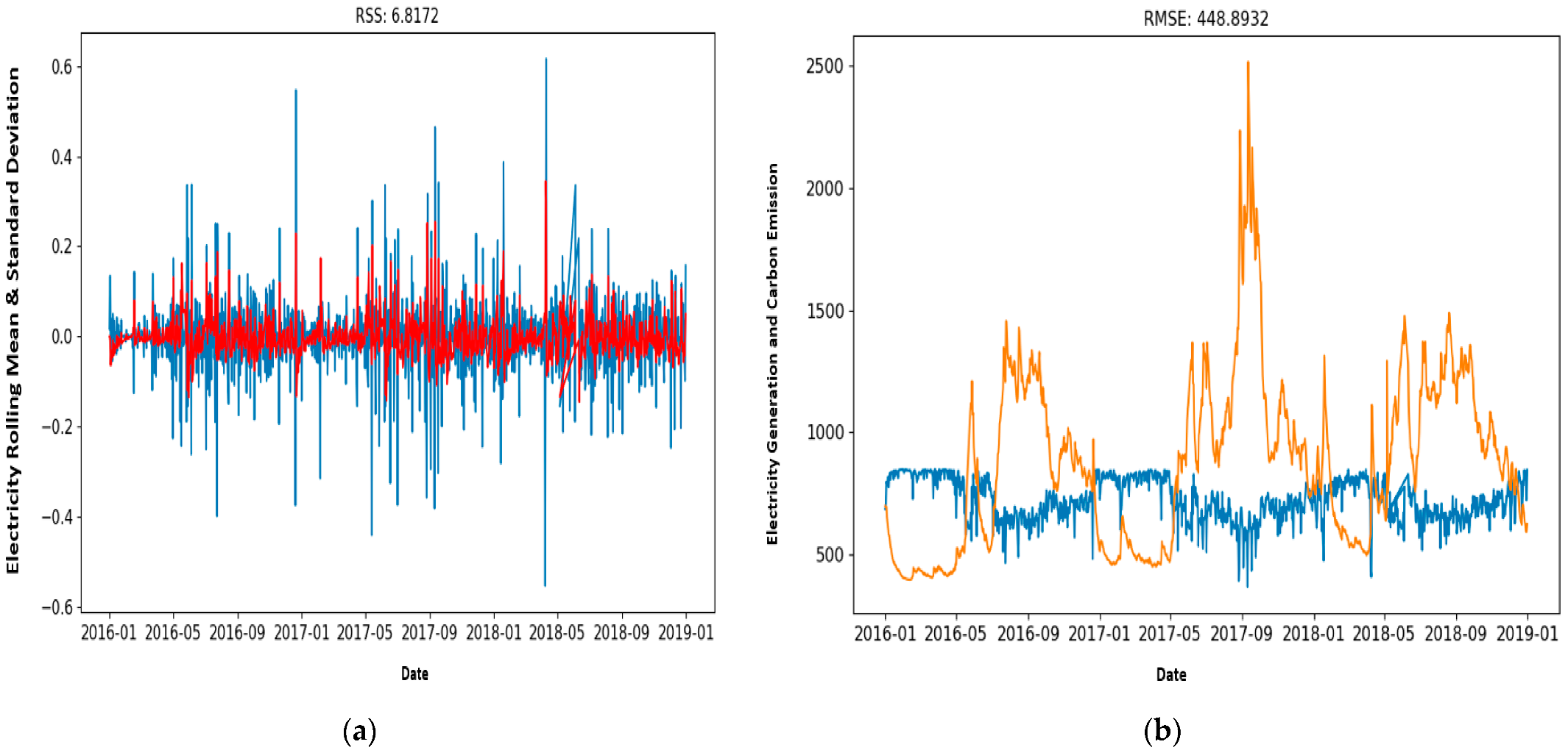
The results of RSS presented in the above graphs for the AR and MA models are 7.6068 and 6.8761, respectively. Combining the difference in the AR and MA results, with integration, resulted in the ARIMA model. The results of the combined models yielded a better result of 6.8172 and RMSE of 448.89. The results of RSS show an improvement of 89.61% for AR and 99.1% for MA. The criterion of parsimony with an RSS value of 6.817284 shows that the model was appropriate for predicting CO2 for five years with a confidence interval of 95%. The identified values of seasonality for the chosen model of (2, 1, 0) (0, 1, 2) proved to be adequate for forecasting carbon emissions for five years with a unit root test statistical procedure employed for the stationarity, while DF was used for the test statistics, scoring −7.5, which was significantly lower than the 1% critical value that is close to stationary. Identification of the model was visualized by inspection of both ACFs and PACFs to determine the possible model use selection in the determination of RSS, to choose the best model.
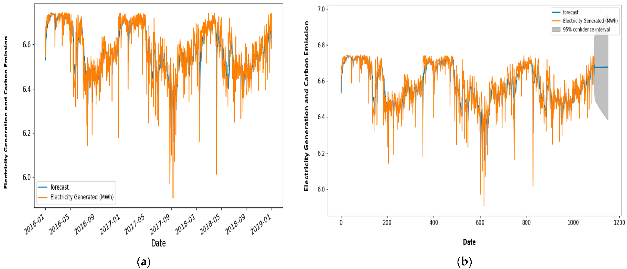
Figure 6 presents test results for autoregressive moving average RSS values for AR and MA models and Figure 7 presents test results for the autoregressive moving average RSS values for ARIMA when combined and the autoregressive moving average RMSE values for ARIMA. In this paper, over 1000 samples were used, leading to reconstruct the error distribution using RMSEs instead of RSS to give a more reliable result.
Figure 8 is the final prediction graph of the predicted values for five years with a confidence interval of 95% for the autoregressive moving average RMSE values for ARIMA, while the grey shape shows the max and min values of CO2 emissions for five years.

5. Discussion

The time-series data obtained for this study provided considerable insight into possible errors associated with data for the prediction model. In this section, comparison with previous studies are proposed to evaluate the likelihood of errors in the obtained data to evaluate the obtained predicted energy consumption and carbon emissions values. Our results were compared with the values of derived carbon emission equivalent using compared country-specific energy according to Intergovernmental Panel on Climate Change (IPCC) emission factors for coal mining. The inherent properties of TS with seasonality trends increase or decrease as variations in the period lead to reconstructing the error distribution using RMSEs instead of RSS to give a more reliable result.
The results are validated by actual data with predicted autoregressive moving average RSS values for ARIMA, when AR and MA is combined, it is confirmed that the proposed prediction model in this study is better judging from the identification of the model, which was visualized by inspection of both ACFs and PACFs in the determination of RSS. This study provides packages that create a pandas library in python, with each representing one of the underlying categories of patterns necessary to see the trend, seasonality, and residual components of our data. The ARIMA library for Python allowed us to set ranges for P, D, and Q values fit the model for possible combinations quickly and perform a grid search to create a model object that fit the training data for manipulating and interpreting variables that depend on time, which can be embedded into a component manufacturing company enterprise system.
The forecasted energy consumption with carbon emissions quantifies the future energy demand of the case company and the reference basis for application of small-scale renewable technologies for some significant energy users (compressed air systems, idling machines wet scrubbers, paint shops, ovens and driers, cooling compressors, chillers and lights). Quantitative energy savings can also be realized with interventions that might include cogeneration plants, and energy efficient measures in companies, which will provide businesses opportunities to prepare for industrial policy implications to be integrated to ensure a balance between manufacturing industry growth and energy efficiency.

6. Conclusions

We have shown that ARIMA models can forecast and predict the electricity generated and carbon emissions for a five-year period based on the previous collected data. The approach is iterative with identification of simple ARIMA models using data plots, autocorrelations, partial autocorrelations, and other information based on estimated appropriate values. As a quantitative approach, TS uses error patterns associated with historical values to predict the electricity demand and CO2 emissions for future transport manufacturing. We used a statistical approach (ARIMA) in this paper to determine the baseline demand for future transport manufacturing and electricity generated TS data for CO2 emissions taking into consideration the errors that may generate incremental or decremental demand. We tracked the errors to train the ARIMA model to improve forecasting accuracy. The concept of demand intelligence is key to the determination of errors from historical data to for accurate prediction of CO2 for effective mitigation and reduction according to climate change targets. The proposed model will help to reduce CO2 emissions as is required for continuous improvement in technologies, invest in innovative energy and resource efficiency, set up initiatives aimed at a reduction in greenhouse gas emissions, and contribute to climate science research. Further studies will focus on the integration of prediction of energy and carbon emission efficiency into a data monitoring device for web and mobile applications for future transport manufacturing industries.

Author Contributions

Conceptualization, R.K.M. and O.T.A.; methodology, R.K.M.; software, O.T.A.; validation, R.K.M. and O.T.A. and K.M.; formal analysis, R.K.M. and O.T.A.; investigation, O.T.A.; resources, R.K.M. and O.T.A.; data O.T.A. and editing, K.M.; visualization, O.T.A.; supervision, O.T.A. and K.M.; project administration, R.K.M.; funding acquisition, K.M. All authors have read and agreed to the published version of the manuscript.

Funding

This research was funded by National Research Foundation (NRF), grant number “123575” and “the APC was funded by the Research Chair in Future Transport Manufacturing Technologies”.

Data Availability Statement

Not applicable.

Acknowledgments

The researchers acknowledge the support and assistance of the Industrial Engineering department of Tshwane University of Technology, Gibela Rail and the National Research Foundation (123575) of South Africa for their financial and material assistance towards executing this research project. The opinions presented in this paper are those of the authors and not the funders.

Conflicts of Interest

The authors declare no conflict of interest.

References

  1. Fahmy-Abdullah, M.; Ismail, R.; Sulaiman, N.; Abdul Talib, B. Technical efficiency in transport manufacturing firms: Evidence from Malaysia. Asian Acad. Manag. J. 2017, 22, 57–77. [Google Scholar] [CrossRef]
  2. Parisa Javadi, P.; Yeganeh, B.; Maryam, A.; Shima, A. Energy assessment and greenhouse gas predictions in the automotive manufacturing industry in Iran. Sustain. Prod. Consum. 2021, 26, 316–330. [Google Scholar] [CrossRef]
  3. IDC. Developing a Vibrant ESCO Market—Prospects for South Africa’s Energy Efficiency Future; I.D. Corporation, Ed.; IDC: Needham, MA, USA, 2018. [Google Scholar]
  4. AIEC. South Africa-Automotive Export Manual 2019; Automotive Industry Export Council: South Africa, 2019; Available online: https://aiec.co.za/downloads/AutomotiveExportManual.pdf (accessed on 6 November 2021).
  5. NAAMSA. South African Economy Manufacturing Presence. 2021. 4. Available online: https://naamsa.net/sa-economy-2021-manufacturing-presence/ (accessed on 6 November 2021).
  6. Jibhakate, R.A.; Nirwan, N.W.; Rambhad, K.S. Enhancing the effectiveness of green technology in manufacturing industry. Mater. Today Proc. 2021, 47, 4298–4305. [Google Scholar] [CrossRef]
  7. Al-Tarawneh, H.A. The Main Factors beyond Decision Making. J. Manag. Res. 2011, 4. [Google Scholar] [CrossRef] [Green Version]
  8. Sallehuddin, R.; Shamsuddin, S.M.; Mohd Hashim, S.Z.; Abraham, A. Forecasting time series data using hybrid grey relational artificial neural network and auto regressive integrated moving average model. Neural Netw. World 2007, 17, 573–605. [Google Scholar]
  9. Sundarakani, B.; de Souza, R.; Goh, M.; Wagner, S.M.; Manikandan, S. Modeling carbon footprints across the supply chain. Int. J. Prod. Econ. 2010, 128, 43–50. [Google Scholar] [CrossRef]
  10. Rehman, H.U.; Rafique, R.; Nasir, M.; Zahid Chudhery, M.A. Forecasting CO2 Emissions from Energy, Manufacturing and Transport Sectors in Pakistan: Statistical Vs. Machine Learning Methods. SSRN J. 2018. Available online: https://papers.ssrn.com/sol3/papers.cfm?abstract_id=3292279 (accessed on 6 November 2021).
  11. Khandelwal, I.; Adhikari, R.; Verma, G. Time Series Forecasting Using Hybrid ARIMA and ANN Models Based on DWT Decomposition. Procedia Comput. Sci. 2015, 48, 173–179. [Google Scholar] [CrossRef] [Green Version]
  12. Chou, J.S.; Trans, D. Forecasting energy consumption time series using machine learning techniques based on usage patterns of residential householders. Energy 2018, 165 Pt B, 709–726. [Google Scholar] [CrossRef]
  13. Hornik, K.; Stinchcombe, M.; White, H. Multilayer feedforward networks are universal approximators. Neural Netw. 1989, 2, 359–366. [Google Scholar] [CrossRef]
  14. Kandananond, K. Forecasting Electricity Demand in Thailand with an Artificial Neural Network Approach. Energies 2011, 4, 1246–1257. [Google Scholar] [CrossRef]
  15. Qi, X.; Chen, G.; Li, Y.; Cheng, X.; Li, C. Applying Neural-Network-Based Machine Learning to Additive Manufacturing: Current Applications, Challenges, and Future Perspectives. Engineering 2019, 5, 721–729. [Google Scholar] [CrossRef]
  16. Gupta, D.; Pratama, M.; Ma, Z.; Li, J.; Prasad, M. Financial time series forecasting using twin support vector regression. PLoS ONE 2019, 14, e0211402. [Google Scholar] [CrossRef]
  17. Khashei, M.; Bijari, M. A New Hybrid Methodology for Nonlinear Time Series Forecasting. Model. Simul. Eng. 2011, 2011, 379121. [Google Scholar] [CrossRef] [Green Version]
  18. Kant, G.; Sangwan, K.S. Predictive Modelling for Energy Consumption in Machining Using Artificial Neural Network. Procedia CIRP 2015, 37, 205–210. [Google Scholar] [CrossRef]
  19. Saleh, C.; Dzakiyullah, N.R.; Nugroho, J.B. Carbon dioxide emission prediction using support vector machine. IOP Conf. Ser. Mater. Sci. Eng. 2016, 114, 012148. [Google Scholar] [CrossRef]
  20. Sen, P.; Roy, M.; Pal, P. Application of ARIMA for forecasting energy consumption and GHG emission: A case study of an Indian pig iron manufacturing organization. Energy 2016, 116, 1031–1038. [Google Scholar] [CrossRef]
  21. Shan, K.; Fan, C.; Wang, J. Model predictive control for thermal energy storage assisted large central cooling systems. Energy 2019, 179, 916–927. [Google Scholar] [CrossRef]
  22. Goudarzi, S.; Anisi, H.; Kama, N.; Doctor, F. Predictive Modelling of Building Energy Consumption based on a Hybrid Nature-Inspired Optimization Algorithm. Energy Build. 2019, 196, 83–93. [Google Scholar] [CrossRef]
  23. Ji, L.; Zou, Y.; He, K.; Zhu, B. Carbon futures price forecasting based with ARIMA-CNN-LSTM model. Procedia Comput. Sci. 2019, 162, 33–38. [Google Scholar] [CrossRef]
  24. Fan, D.; Sun, H.; Yao, J.; Zhang, K. Well production forecasting based on ARIMA-LSTM model considering manual operations. Energy 2020, 220, 119708. [Google Scholar] [CrossRef]
  25. Box, G.E.; Jenkins, G.M.; Reinsel, G.C.; Ljung, G.M. Time Series Analysis: Forecasting and Control; John Wiley & Sons: Hoboken, NJ, USA, 2015. [Google Scholar]
  26. Giampieri, A.; Ling-Chin, J.; Ma, Z.; Smallbone, A.; RoskillY, A.P. A review of the current automotive manufacturing practice from an energy perspective. Appl. Energy 2020, 261, 114074. [Google Scholar] [CrossRef]
  27. Kumar, R.; Lamba, K.; Raman, A. Role of zero emission vehicles in sustainable transformation of the Indian automobile industry. Res. Transp. Econ. 2021, 101064, in press. [Google Scholar] [CrossRef]
  28. Aggelakakis, A.; Bernardino, J.; Boile, M.; Christidis, P.; Condeco Melhorado, A.; Krail, M.; Papanikolaou, A.; Reichenbach, M.; Schippl, J. The future of the transport industry. Publications Office of the European Union: Luxembourg EUR 27085. JRC93544. Available online: https://publications.jrc.ec.europa.eu/repository/handle/JRC93544 (accessed on 6 November 2021).
  29. USDOE. Technology Roadmap for Energy Reduction in Automotive Manufacturing; USDOE, Ed.; 2008; pp. 1–81. Available online: https://www1.eere.energy.gov/manufacturing/intensiveprocesses/pdfs/auto_industry_roadmap.pdf (accessed on 6 November 2021).
  30. Yang, H.K.; Bukkapatnam, S.; Satish, T.; Fugee, S.T. The internet of things for smart manufacturing: A review. IISE Trans. 2019, 51, 1190–1216. [Google Scholar] [CrossRef]
  31. Kusiak, A. Smart manufacturing. Int. J. Prod. Res. 2017, 56, 508–517. [Google Scholar] [CrossRef]
  32. NCPC. Results and Impact in the Automotive Sector; N.C.P. Centre, Ed.; 2013; pp. 1–40. Available online: http://www.gcpcenvis.nic.in/PDF/Energy_Efficiency_Results_Impact_in_the_Automotive_Sector.pdf (accessed on 6 November 2021).
  33. DEA. National Climate Change Response White Paper. 2016; pp. 1–50. Available online: https://www.gov.za/sites/default/files/gcis_document/201409/nationalclimatechangeresponsewhitepaper0.pdf (accessed on 6 November 2021).
  34. DEA. The South African Energy Sector Report. 2019. Available online: http://www.energy.gov.za/files/media/explained/2019-South-African-Energy-Sector-Report.pdf (accessed on 6 November 2021).
  35. Nedbank. The Energy Efficiency Guide; Nedbank: Thornton, South Africa, 2017; Available online: https://www.nedbank.co.za/content/nedbank/desktop/gt/en/aboutus/green-and-caring/Publications/the-energy-efficiency-guide.html (accessed on 6 November 2021).
  36. Ramos, D.; Faria, P.; Vale, Z.; Mourinho, J.; Correia, R. Industrial Facility Electricity Consumption Forecast Using Artificial Neural Networks and Incremental Learning. Energies 2020, 13, 4774. [Google Scholar] [CrossRef]
  37. Liu, W.; Peng, T.; Kishita, Y.; Umeda, Y.; Tang, R.; Tang, W.; Hu, L. Critical life cycle inventory for aluminum die casting: A lightweight-vehicle manufacturing enabling technology. Appl. Energy 2021, 304, 117814. [Google Scholar] [CrossRef]
  38. Fysikopoulos, A.; Anagnostakis, D.; Salonitis, K.; Chryssolouris, G. An Empirical Study of the Energy Consumption in Automotive Assembly. Procedia CIRP 2012, 3, 477–482. [Google Scholar] [CrossRef] [Green Version]
  39. Du Plessis, W. Energy efficiency and the law: A multidisciplinary approach. S. Afr. J. Sci. 2015, 111, 1–8. [Google Scholar] [CrossRef] [Green Version]
  40. Kluczek, A. An energy-led sustainability assessment of production systems—An approach for improving energy efficiency performance. Int. J. Prod. Econ. 2019, 216, 190–203. [Google Scholar] [CrossRef]
  41. Thollander, P.; Danestig, M.; Rohdin, P. Energy policies for increased industrial energy efficiency: Evaluation of a local energy programme for manufacturing SMEs. Energy Policy 2007, 35, 5774–5783. [Google Scholar] [CrossRef] [Green Version]
  42. Malinauskaite, J.; Jouhara, H.; Ahmad, L.; Milani, M.; Montorsi, L.; Venturelli, M. Energy efficiency in industry: EU and national policies in Italy and the UK. Energy 2019, 172, 255–269. [Google Scholar] [CrossRef]
  43. Bonilla, I.; Nieto, N.; Portillo-Valdés, L.; Egilegor, B. Energy efficiency assessment: Process modelling and waste heat recovery analysis. Energy Convers. Manag. 2019, 196, 1180–1192. [Google Scholar] [CrossRef]
  44. Rue du Can, D.S.; Pudleiner, D.; Pielli, K. Energy efficiency as a means to expand energy access: A Uganda roadmap. Energy Policy 2018, 120, 354–364. [Google Scholar] [CrossRef]
  45. Gomez Chavez, K.M. Energy Efficiency in Wireless Access Networks: Measurements, Models and Algorithms. Ph.D. Thesis, University of Trento, Trento, Italy, 2013. [Google Scholar]
  46. Xiong, S.; Ma, X.; Ji, J. The impact of industrial structure efficiency on provincial industrial energy efficiency in China. J. Clean. Prod. 2019, 215, 952–962. [Google Scholar] [CrossRef]
  47. Pretorius, I.; Piketh, S.J.; Burger, R.P. The Impact of the South African energy Crisis on Emissions. In Air Pollution XXIII; 2015; pp. 255–264. Available online: https://www.researchgate.net/profile/Roelof-Burger/publication/283097663_The_impact_of_the_south_african_energy_crisis_on_emissions/links/56e1381708aee77a15feae92/The-impact-of-the-south-african-energy-crisis-on-emissions.pdf (accessed on 6 November 2021).
  48. Meng, Z.; Wang, H.; Wang, B. Empirical Analysis of Carbon Emission Accounting and Influencing Factors of Energy Consumption in China. Int. J. Environ. Res. Public Health 2018, 15, 2467. [Google Scholar] [CrossRef] [Green Version]
  49. Kunda, D.; Phiri, H. An Approach for Predicting CO2 Emissions using Data Mining Techniques. Int. J. Comput. Appl. 2017, 172, 7–10. [Google Scholar] [CrossRef]
  50. Benedetti, M.C.; Vittorio, I.V. Improving Energy Efficiency in Manufacturing Systems—Literature Review and Analysis of the Impact on the Energy Net-work of Consolidated Practices and Upcoming Opportunities. Energy Efficiency Improvements in Smart Grid Components-IntechOpen Book Series. 2015. Available online: https://www.researchgate.net/profile/Vito-Introna/publication/292124754_Improving_Energy_Efficiency_in_Manufacturing_Systems_-_Literature_Review_and_Analysis_of_the_Impact_on_the_Energy_Network_of_Consolidated_Practices_and_Upcoming_Opportunities/links/5756b5b608ae0405a5782d08/Improving-Energy-Efficiency-in-Manufacturing-Systems-Literature-Review-and-Analysis-of-the-Impact-on-the-Energy-Network-of-Consolidated-Practices-and-Upcoming-Opportunities.pdf (accessed on 6 November 2021).
  51. Schleich, J.; Fleiter, T. Effectiveness of energy audits in small business organizations. Resour. Energy Econ. 2019, 56, 59–70. [Google Scholar] [CrossRef]
  52. Javied, T.; Rackow, T.; Franke, J. Implementing Energy Management System to Increase Energy Efficiency in Manufacturing Companies. Procedia CIRP 2015, 26, 156–161. [Google Scholar] [CrossRef] [Green Version]
  53. Flick, D.; Ji, L.; Dehning, P.; Thiede, S.; Herrmann, C. Energy Efficiency Evaluation of Manufacturing Systems by Considering Relevant Influencing Factor. Procedia CIRP 2017, 63, 586–591. [Google Scholar] [CrossRef]
  54. Apostolos, F.; Alexios, P.; Georgios, P. Energy efficiency of manufacturing processes: A critical review. Procedia CIRP 2013, 7, 628–633. [Google Scholar] [CrossRef] [Green Version]
  55. Diaz C, J.L.; Ocampo-Martinez, C. Energy efficiency in discrete-manufacturing systems: Insights, trends, and control strategies. J. Manuf. Syst. 2019, 52, 131–145. [Google Scholar] [CrossRef] [Green Version]
  56. Adenuga, O.T.; Mpofu, K.; Ramatsetse, B. Energy efficiency analysis modelling system for manufacturing in the context of industry 4.0. Procedia CIRP 2019, 80, 735–740. [Google Scholar] [CrossRef]
  57. May, G.A.; Dimitris, K. Business Model for Energy Efficiency in Manufacturing. Procedia CIRP 2017, 61, 410–415. [Google Scholar] [CrossRef]
  58. Mawson, V.J.; Hughes, B.R. The development of modelling tools to improve energy efficiency in manufacturing processes and systems. J. Manuf. Syst. 2019, 51, 95–105. [Google Scholar] [CrossRef]
  59. Heo, Y.; Zavala, V.M. Gaussian process modeling for measurement and verification of building energy savings. Energy Build. 2012, 53, 7–18. [Google Scholar] [CrossRef]
  60. Lee, K.H. Carbon accounting for supply chain management in the automobile industry. J. Clean. Prod. 2012, 36, 83–93. [Google Scholar] [CrossRef]
  61. Siltonen, S. Implication of Energy Efficiency Improvement for CO2 Emission in Energy-Intensive Industry. Doctoral Dissertation, Aalto University, Espoo and Helsinki, Finland, 2010. [Google Scholar]
  62. Dufour, T.; Hoang, H.M.; Oignet, J.; Osswald, V.; Fournaison, L.; Delahaye, A. Experimental and modelling study of energy efficiency of CO2 hydrate slurry in a coil heat exchanger. Appl. Energy 2019, 242, 492–505. [Google Scholar] [CrossRef]
  63. Lee, S.; Chong, W.O. Causal relationships of energy consumption, price, and CO2 emissions in the U.S. building sector. Resour. Conserv. Recycl. 2016, 107, 220–226. [Google Scholar] [CrossRef]
  64. Jalil, A.; Rao, N.H. Time Series Analysis (Stationarity, Cointegration, and Causality). In Environmental Kuznets Curve (EKC), Chapter 8; Özcan, B., Öztürk, I., Eds.; Academic Press: Cambridge, MA, USA, 2019; pp. 85–99. [Google Scholar]
  65. Deb, C.; Zhang, F.; Yang, J.; Lee, S.E.; Shah, K.W. A review on time series forecasting techniques for building energy consumption. Renew. Sustain. Energy Rev. 2017, 74, 902–924. [Google Scholar] [CrossRef]
  66. Pao, H.T.; Fu, H.C.; Tseng, C.L. Forecasting of CO2 emissions, energy consumption and economic growth in China using an improved grey model. Energy 2012, 40, 400–409. [Google Scholar] [CrossRef]
  67. Lotfalipour, M.R.; Falahi, M.A.; Bastam, M. Prediction of CO2 emission in Iran using grey and ARIMA models. Int. J. Energy Econ. Policy 2013, 3, 9. [Google Scholar]
  68. Wang, X.; Meng, M. A Hybrid Neural Network and ARIMA Model for Energy Consumption Forcasting. J. Comput. 2012, 7, 1184–1190. [Google Scholar] [CrossRef]
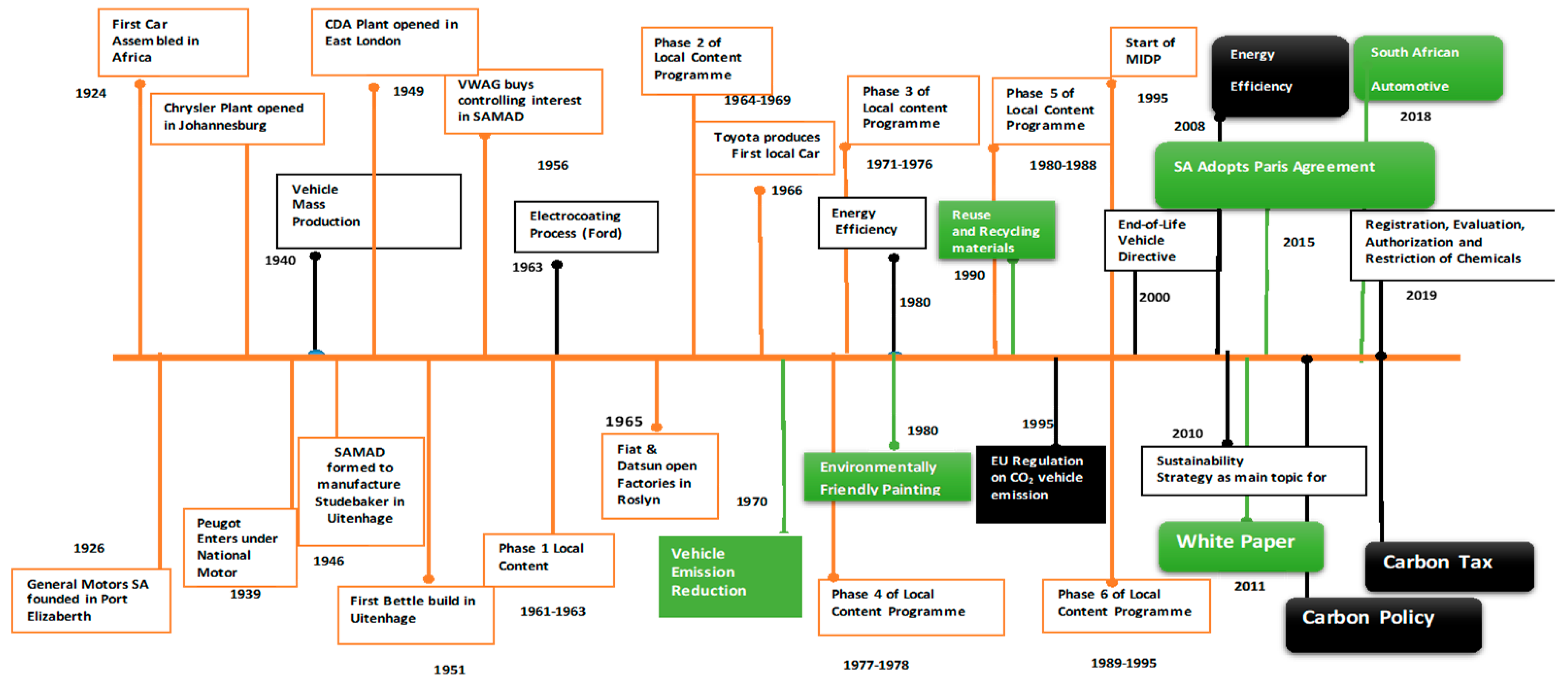
Figure 1. Global and South African automotive revolution began in 1924, with emergence of energy consumption and carbon emission regulations (Source Authors).
Energies 14 08466 g001
Figure 2. Steps for ARIMA model selection.
Energies 14 08466 g002
Figure 3. Test results (a) based on the original data, and the (b) overall increasing trend in the data along with some seasonal variations.
Energies 14 08466 g003
Figure 4. Test results: (a) pre−estimation, eliminating trend and seasonality; (b) post−estimation, eliminating trend and seasonality.
Energies 14 08466 g004
Figure 5. Test results: (a) autocorrelation (b) partial autocorrelation.
Energies 14 08466 g005
Figure 6. Test results: (a) autoregressive moving average RSS values for AR and (b) autoregressive moving average RSS values for the MA model.
Energies 14 08466 g006
Figure 7. Test results: (a) autoregressive moving average RSS values for ARIMA when combined and (b) autoregressive moving average RMSE values for ARIMA.
Energies 14 08466 g007
Figure 8. Test results: (a) autoregressive moving average RMSE values for ARIMA and (b) autoregressive moving average RMSE values for ARIMA with the predicted values for five years.
Energies 14 08466 g008
Table 1. Electricity generated and carbon emission data.
PeriodDurationElectricity Generated
(MWh)
Carbon
Emissions
(tons)
PeriodDurationElectricity Generated
(MWh)
Carbon
Emissions
(tons)
Jan 20163125,383.917,991Jul 20173121,31415,991
Feb 20162924,091.416,999Aug 20173119,38714,545
Mar 20163125,732.718,157Sept 20173017,52213,146
Apr 20163024,849.917,534Oct 20173121,60716,211
May 20161511,679.28241Nov 20173019,18414,393
Jun 20163020,346.114,356Dec 20173122,32816,751
Jul 20163119,938.914,069Jan 20183122,09516,576
Aug 20163119,863.114,015Feb 20182822,08616,570
Sep 20163018,708.013,753Mar 20183125,05318,796
Oct 20163121,797.616,354Apr 20183022,06516,554
Nov 2016302088.315,667May 2018644873367
Dec 20163123,259.317,450Jun 20182014,30810,735
Jan 20173125,219.418,921Jul 20183120,44615,339
Feb 20172822,019.016,519Aug 20183120,05715,047
Mar 20173125,443.019,089Sept 20183019,57514,686
Apr 20173024,410.718,314Oct 20183121,55616,173
May 20172718,93514,206Nov 20183021,69016,273
Jun 20171380886068Dec 20183123,72617,800
Table 2. Initial Dickey–Fuller test of the original data.
DescriptionOriginal DataPost-Estimating and Eliminating TrendsPost-Eliminating Trend and Seasonality
Test statistic−3.602352−9.397422−7.793783
p-value0.0057166.319227.815122
Number of #lags used61.58
Number of observations used1086.000001.0661.084
Critical value (1%)−3.436386−3.436499−3.46397
Critical value (5%)−2.864205−2.864255−2.86421
Critical value (10%)−2.568189−2.568216−2.568961
Publisher’s Note: MDPI stays neutral with regard to jurisdictional claims in published maps and institutional affiliations.