Article

Constant Voltage Model of DFIG-Based Variable Speed Wind Turbine for Load Flow Analysis

Department of Electrical Engineering, Tanjungpura University, Pontianak 78124, Indonesia
Energies 2021, 14(24), 8549; https://doi.org/10.3390/en14248549
Submission received: 24 November 2021 / Revised: 10 December 2021 / Accepted: 16 December 2021 / Published: 18 December 2021
(This article belongs to the Special Issue Power System Modeling, Analysis and Simulation)

Abstract

:
At present, the penetration of wind-driven electric generators or wind power plants (WPPs) in electric power systems is getting more and more extensive. To evaluate the steady state performances of such power systems, developing a valid WPP model is therefore necessary. This paper proposes a new method in modeling the most popular type of WPP, i.e., DFIG (doubly fed induction generator)-based WPP, to be used in power system steady state load flow analysis. The proposed model is simple and derived based on the formulas that calculate turbine mechanical power and DFIG power. The main contribution of the paper is that, in contrast to the previous models where the DFIG power factor has been assumed to be constant at unity, the constant voltage model proposed in this paper allows the power factor to vary in order to keep the voltage at the desired value. Another important contribution is that the proposed model can be implemented in both sub-synchronous and super-synchronous conditions (it is to be noted that most of the previous models use two different mathematical models to represent the conditions). The case study is also presented in the present work, and the results of the study confirm the validity of the proposed DFIG model.

1. Introduction

The application of variable speed wind turbines for electricity generation has been increasing in recent years. This increasing application is mainly because a variable speed WPP can extract wind energy in a more optimal way than a fixed speed WPP. Variable speed operation of a WPP can be achieved through the use of DFIG or PMSG (permanent magnet synchronous generator) as its main energy converter. However, currently, the DFIG application is more popular because it costs less than PMSG [1,2]. In the operation of the DFIG, two different control modes (i.e., power factor control mode and voltage control mode) are often adopted. In power factor control mode, the DFIG power factor is kept constant during operation, while the voltage magnitude varies within allowable limits. On the other hand, in voltage control mode, the voltage magnitude is kept constant, and the DFIG power factor is allowed to vary to keep the voltage at desired value [3,4,5,6].
To be able to study or analyze power systems embedded with WPP, modeling of the power system components, including the WPP, is necessary. In power system load flow analysis, a traditional power plant is usually modeled as a PV bus model. However, since the WPP does not have the capability of controlling active power output, this PV bus model is no longer applicable for WPP. Therefore, in order that the analysis can properly be carried out and the system steady state performances can correctly be assessed, formulation and development of the WPP model are necessary.
In the context of WPP steady state load flow model, several interesting techniques have been proposed. References [4,5,6,7,8,9,10,11,12,13,14,15,16,17,18], for example, report some of the recent methods. In [7,8,9], multiple-node models of asynchronous generator-based WPP for load flow analysis are proposed. By applying the proposed methods in [7,8,9], a conventional load flow solver can be employed to solve the load flow problem. However, input data to the load flow solver needs to be modified to incorporate the WPP data. References [10,11,12,13,14,15] discuss various steady state models of fixed speed WPP for load flow analysis. In the method [10,11,12,13,14,15], the developed mathematical model is combined with the load flow formulation of a system without WPP. The combined equations are then simultaneously solved using some iterative techniques to obtain the solution to the load flow problem.
References [4,5,6,16,17,18] propose several models of DFIG-based WPP for load flow analysis. In [4], a three-phase model of DFIG to be used in unbalanced distribution system load flow (DSLF) analysis is proposed. Reference [5] proposes an iterative technique to integrate DFIG in load flow analysis. The proposed model in [5] is developed based on the DFIG equivalent circuit. In [6], a framework for incorporating DFIG-based WPP in load flow analysis of distribution systems has been proposed. The proposed model in [6] is also developed based on the DFIG equivalent circuit, and the forward–backward sweep technique has been employed to obtain the load flow solution. A steady-state model of DFIG-based variable speed WPP for three-phase load flow analysis is investigated and presented in [16]. The sequence components theory has been used in deriving the proposed model. Refs. [17,18] proposes a simple technique for modeling DFIG-based WPP to be used in power system steady-state load flow studies. Development of the WPP model in [17,18] is carried out based only on power formulations of the WPP. Table 1 summarizes the previously published models of DFIG-based WPP for load flow analysis.
In this paper, a new steady state model of DFIG-based WPP for load flow analysis is proposed. Similar to the model in [17,18], in the present work, derivation of the proposed mathematical model is also based on the DFIG power formulas and turbine mechanical power formula. The process of the model development is relatively straightforward, and therefore, the resulted model is quite simple and can easily be incorporated into the power system load flow analysis. The main contributions of the present work can be described as follows: (i) In contrast to the model in [4,5,6,16,17,18], where DFIG power factor has been assumed to be constant at unity, the constant voltage model proposed in this paper allows the power factor to vary to keep the voltage at the desired value; (ii) The proposed model can be implemented in both sub-synchronous and super-synchronous conditions (it is to be noted that references [5,6,16] use two different mathematical models to represent the conditions).

2. DFIG-Based WPP

The basic structure of a DFIG-based WPP is shown in Figure 1 [3,17,18,19,20,21]. In Figure 1, Pm is turbine power, PS and QS are stator powers, PR and QR are rotor powers, and Pg and Qg are WPP output powers. Moreover, in Figure 1, RSC and GSC stand for rotor side converter and grid side converter, respectively. As mentioned earlier, the DFIG system is normally operated at a constant voltage magnitude or a constant power factor. In constant voltage operation mode, the DFIG terminal voltage magnitude is kept constant during operation. However, in constant power factor operation mode, the DFIG power factor is held constant during operation. In this mode, three power factors (i.e., unity, leading, and lagging power factors) are usually adopted in the operation. In unity power factor mode, the reactive power in the stator of WRIG (wound rotor induction generator) is zero (or Qg = 0); therefore, there is no reactive power exchange between the WPP and power grid. In lagging power factor mode, the DFIG absorbs reactive power from the power grid (or Qg is negative). On the other hand, in leading power factor mode, the DFIG delivers reactive power to the power grid (or Qg is positive), and, consequently, can support the system reactive power demand and voltage profile improvement.
Figure 2 and Figure 3 show the steady state equivalent circuits of WRIG [3,17,18,19,20,21]. To include turbine mechanical power and rotor power in the WRIG equivalent circuit, the equivalent circuits in Figure 2 and Figure 3 are modified to those given in Figure 4 and Figure 5 [3,18,19,20,21,22]. In the figures, VS and IS are stator voltage and current, VR and IR are rotor voltage and current, RS and XS are stator resistance and reactance, RR and XR are rotor resistance and reactance, Rc and Xm are core circuit resistance and reactance, SS is stator complex power, IM is core circuit current, and s is WRIG slip. Based on Figure 4 and Figure 5, the following formulas that calculate turbine mechanical power and rotor power can be shown to be valid:
P m = [ V R I R * R R I R I R * ] 1 s s
and:
P R + j s Q R = V R I R *
where QR is, as mentioned before, the reactive power produced by the DFIG rotor seen from the stator side.
Furthermore, by looking at Figure 1, the WPP active power output is DFIG stator active power minus DFIG rotor power, or:
P g = P S P R
and the WPP reactive power output is:
Q g = Q S
Based on Figure 2, Figure 3, Figure 4 and Figure 5, the electrical power in DFIG stator is:
S S = P S + j Q S = V S I S *

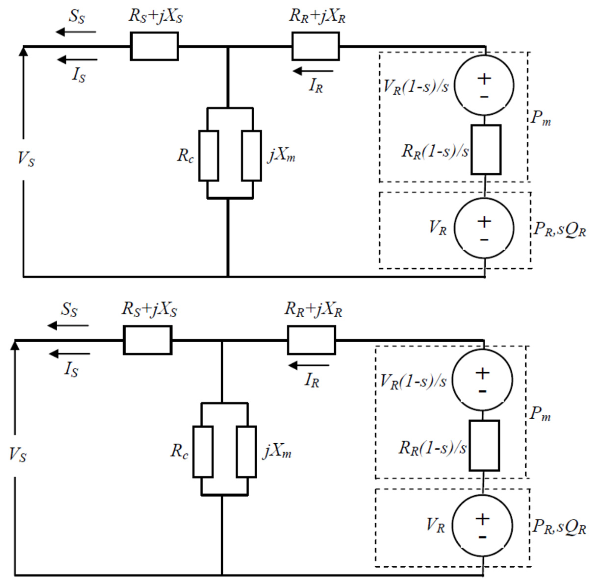
3. Modeling of DFIG-Based WPP

The proposed constant voltage model of DFIG-based WPP will be developed based on the formulas described in Section 2. On using (2) and (3) in (4) and (5), the formulas of WPP active and reactive power outputs become:
P g = R e ( V S I S * ) R e ( V R I R * )
Q g = I m ( V S I S * )
Therefore, based on (1), (2), (6) and (7), the proposed constant voltage model of DFIG-based WPP is:
s P m + ( 1 s ) R R I R I R * ( 1 s ) R e ( V R I R * ) = 0
s Q R I m ( V R I R * ) = 0
P g R e ( V S I S * ) + R e ( V R I R * ) = 0
Q g I m ( V S I S * ) = 0
It is to be noted that IS and IR in (8)–(11) can be expressed in terms of VS and VR (see Appendix A). In the load flow analysis, mathematical model (8)–(11) is then combined with the following nodal equations of system without WPP [23]:
P G i P L i j = 1 n | V i | | Y i j | | V j | c o s ( δ i δ j θ i j ) = 0
Q G i Q L i j = 1 n | V i | | Y i j | | V j | s i n ( δ i δ j θ i j ) = 0
In (12) and (13), PG and QG are power generations, PL and QL are power demands, |V| and δ are voltage magnitude and angle, |Y| and θ are magnitude and angle of bus admittance matrix element, and n is number of system buses. Table 2 gives detail of the equations to be solved as well as the variables to be determined in the complete formulation of load flow analysis for system embedded with DFIG-based WPP. It is to be noted that VS in (10) and (11) is also the voltage at WPP bus (i.e., V = |V|∟δ). In constant voltage mode of operation, the magnitude of this voltage (|V| = |VS|) is known or specified at a certain value.

4. Case Study

4.1. Test System

The case study is based on 5-bus power system with total three phase loads of 1215 MW and 600 MVAR [23]. The system data are given in Table 3 and Table 4. The system is then modified by adding a WPP at bus 5 via a step-up transformer with an impedance of j0.05 pu (see Figure 6). The WPP consists of 100 identical DFIG-based wind turbine generator (WTG) units. Data of the WTG unit are given in Table 5. This WTG unit data is adopted from [18]. Base value of 100 MVA has been used for all data in pu.

4.2. Calculations of Slip and Turbine Power

Machine slip and turbine mechanical power can be calculated using the formulas given in [17]. In the present work, it is assumed that the turbine tip speed ratio (λ) is 8.0, and turbine coefficient performance (CP) is 0.50. Therefore, the mechanical power produced by each turbine is:
P m = 0.5 ( 1.225 ) ( π 40 2 ) V w 3 ( 0.5 )
The machine slip is:
s = 1 ( 2 ) ( 8 ) V w ( 100 π ) ( 1 / 90 ) ( 40 )
Table 6 shows the results of machine slip and turbine mechanical power calculations for three wind speed values (i.e., 8, 9 and 10 m/s). These results (i.e., Pm and s) will be used in the load flow study discussed in Section 4.4.

4.3. WPP Aggregation

To simplify the load flow analysis, the group of WTG units in Figure 6 is aggregated into a single machine equivalent (note: aggregation technique as discussed in [3] has been used in the aggregation process). In the WPP single machine representation (see Figure 7), parameters of the WRIG equivalent are:
R S , e k = 1 / 100 = 0.01   pu
X S , e k = 25 / 100 = 0.25   pu
R R , e k = 1 / 100 = 0.01   pu
X R , e k = 25 / 100 = 0.25   pu
R c , e k = 3000 / 100 = 30   pu
X M , e k = 350 / 100 = 3.5   pu
The impedance of pad mount transformer in the single machine equivalent is:
Z T , e k = j 5 / 100 = j 0.05   pu

4.4. Load Flow Results and Discussion

Using the WPP single machine representation, a load flow study is then carried out for various values of wind speed listed in Table 6. In addition, in the study, the WPP terminal voltages have been specified to some values ranging from 0.95 to 1.0 pu. Results of the study are given in Table 7, Table 8, Table 9, Table 10, Table 11, Table 12, Table 13, Table 14 and Table 15. It is to be noted that the power factors in Table 8, Table 11 and Table 14 are determined after the load flow analysis has been completed, and they are calculated based on the WPP active and reactive power outputs as follows:
P F = c o s ( a   t a n Q g P g )
It can be seen from the tables that all of the power factors are above 0.85, which are considered to be good power factors.
Some of the results in Table 7, Table 8, Table 9, Table 10, Table 11, Table 12, Table 13, Table 14 and Table 15 are also presented in graphical forms (see Figure 8, Figure 9, Figure 10, Figure 11, Figure 12, Figure 13, Figure 14, Figure 15, Figure 16, Figure 17 and Figure 18) to make a better observation. Figure 8 shows the variation of DFIG rotor active power. It can be seen from the figure that DFIG rotor active power (PR) is almost not affected by the improvement of WPP voltage. It can also be seen that, at a wind speed of 8 m/s, the rotor active power is positive, which indicates that the DFIG is at sub-synchronous condition (DFIG rotor absorbs the active power). On the other hand, at wind speeds of 9 and 10 m/s, the rotor active power is negative, which indicates that the DFIG is at super-synchronous condition (DFIG rotor delivers the active power). It is to be noted that the wind speeds of 8, 9, and 10 m/s have been selected in the study to investigate the DFIG in two normal operating conditions, i.e., sub- and super-synchronous conditions. Only those three values are chosen because they already represent the conditions.
As mentioned before, the DFIG rotor active power (PR) is almost not affected by the improvement of WPP voltage. However, this is not the case for the reactive power produced by the DFIG rotor (QR). The DFIG rotor reactive power is significantly increased with the improvement of WPP voltage magnitude (see Figure 9). This result is expected since more reactive power is needed to obtain a better voltage profile. Power loss in DFIG is also increasing when the WPP voltage goes up (see Figure 10 and Figure 11). The DFIG power loss is calculated using the formula given in Appendix B. This increase in power loss is due to the rise in WRIG currents as the WPP voltage magnitude is raised. As a result, the increase in DFIG active power loss will, therefore, slightly decrease the WRIG stator active power (PS) and WPP active power output (PG), as shown in Figure 12 and Figure 13. On the other hand, as the reactive power produced by the DFIG rotor is significantly increased, the WPP reactive power output (QG) will also be higher as the WPP voltage magnitude is improved (see Figure 14). This result is also expected, since part of the DFIG rotor reactive power is delivered to the power grid to support the system reactive power demand and voltage improvement.
The active power output of a conventional power plant (G1+G2) is almost not affected by the improvement of WPP voltage (see Figure 15). However, since some portions of system reactive power demand can be supplied by the WPP, the reactive power output of the conventional power plant can therefore be reduced as the WPP terminal voltage increases (see Figure 16). Furthermore, as can be seen from Figure 17 and Figure 18, which show the variation of transmission line power losses, the increase in WPP voltage will reduce the line power losses. It is to be noted that the line loss is proportional to the square of the current flowing in the line. Since the improvement in voltage profile causes the line voltage drop (i.e., the current flowing in the line) to be smaller, the line power loss can therefore be significantly reduced.
From the above results, two important observations regarding the novelty of the main findings can be described as follows. Firstly, the proposed method works well at various specified voltage levels. The DFIG power factors are allowed to vary from lagging to leading power factors to keep the voltage at the specified magnitude. It is to be noted that the DFIG power factor has been assumed constant at unity in most of the previously published methods. Secondly, the proposed model is able to perform properly at both DFIG sub- and super-synchronous speeds. In contrast, some of the previous methods used two different equations to model the DFIG in sub- and super-synchronous conditions. The results also show that with the installation of DFIG-based WPP, in terms of power system steady-state performance, the following advantages can be obtained:
(i)
The improvement in system voltage profile leads to the reduction in transmission line power loss. In turn, this loss reduction will lower the power system operational cost and increase the system efficiency.
(ii)
The decrease in power supply from conventional electric generators. Conventional electric generators are usually fossil fuel-based power plants that are not environmentally friendly. This advantage will, therefore, help in coping with the global climate change issues.

5. Conclusions

In this paper, a new steady state model of DFIG-based WPP for load flow analysis has been proposed. In the present work, the derivation of the proposed mathematical model is based on the formulas that calculate turbine mechanical power and DFIG power. The process of the model development is relatively straightforward; therefore, the resulted model is quite simple and can easily be incorporated into the power system load flow analysis. The main contributions of the paper are:
  • In contrast to the previous models, where DFIG power factor has been assumed to be constant at unity, the constant voltage model proposed in this paper allows the power factor to vary to keep the voltage at the specified value. In the present work, various DFIG voltage magnitudes ranging from 0.95 to 1.0 pu have been investigated, and the power factors vary from 0.98 lagging to 0.98 leading.
  • The proposed model can be implemented in both sub-synchronous and super-synchronous conditions (it is to be noted that most of the previous models use two different mathematical models to represent the conditions). Three wind speed values (i.e., 8, 9, and 10 m/s) have been studied in this paper. At a wind speed of 8 m/s, the DFIG rotor active power is positive, which indicates that the DFIG is at sub-synchronous condition (DFIG rotor absorbs the active power). On the other hand, at wind speeds of 9 and 10 m/s, the DFIG rotor active power is negative, which indicates that the DFIG is at super-synchronous condition (DFIG rotor delivers the active power).
Case study results confirm the validity of the proposed DFIG model. However, the method in the present work can only be applied to DFIG-based WPP in voltage control mode. In future work, modification of the method so that it can be applied to DFIG-based WPP in power factor control mode can be investigated. This is an interesting research area since the power factor control mode is also often adopted in the operation of DFIG-based WPP.

Funding

This research was funded by Kemendikbud-Ristek Republik Indonesia, grant number: 156/E4.1/AK.04.PT/2021.

Institutional Review Board Statement

Not applicable.

Informed Consent Statement

Not applicable.

Data Availability Statement

Not applicable.

Conflicts of Interest

The author declares no conflict of interest.

Appendix A

By examining Figure 3, the current in magnetic circuit can be formulated as:
I M = 1 s Z M V R Z R Z M I R
or:
I M = 1 Z M V S + Z S Z M I S
On using Kirchhoff current law in circuit of Figure 3, the following relationship can be obtained:
I S I R + I M = 0
Based on (A3), the stator current:
I S = I R I M
and rotor current:
I R = I S + I M
Substituting (A1) into (A4), stator current becomes:
I S = ( 1 + Z R Z M ) I R 1 s Z M V R
In the same way, substituting (A2) into (A5), rotor current becomes:
I R = ( 1 + Z S Z M ) I S + 1 Z M V S
On using Kirchhoff voltage law in circuit of Figure 3, the following relationship can also be obtained:
V S V R s + Z S I S + Z R I R = 0
Based on (A8), the alternative formula for stator current is:
I S = 1 s Z S V R 1 Z S V S Z R Z S I R
and that for rotor current:
I R = 1 s Z R V R 1 Z R V S Z S Z R I S
By substituting (A10) into (A6) and (A9) into (A7), it can be shown that the stator and rotor currents can be expressed in terms of stator and rotor voltages as follows:
I S = 1 s ( Z S + Z R + Z S Z R Z M ) V R 1 + Z R / Z M Z S + Z R + Z S Z R Z M V S
I R = 1 + Z S / Z M s ( Z S + Z R + Z S Z R Z M ) V R 1 Z S + Z R + Z S Z R Z M V S
In a more compact form, (A11) and (A12) can be rewritten as:
I S = E V R F V S
I R = G V R H V S
where:
E = 1 s ( Z S + Z R + Z R Z S / Z M )
F = 1 + Z R / Z M Z S + Z R + Z R Z S / Z M
G = 1 + Z S / Z M s ( Z S + Z R + Z R Z S / Z M )
H = 1 Z S + Z R + Z R Z S / Z M

Appendix B

By looking at Figure 5, power loss in WRIG is:
S l o s s = I S I S * Z S + I R I R * Z R R + I M I M * Z M
Since the magnetic circuit current:
I M = I R I S
Then, on using (A17) in (A16), the WRIG power loss will become:
S l o s s = I S I S * ( Z S + Z M ) + I R I R * ( Z R R + Z M ) ( I R I S * + I S I R * ) Z M
where IS and IR are calculated using (A13) and (A14), respectively.

References

  1. Anaya-Lara, O.; Jenkins, N.; Ekanayake, J.B.; Cartwright, P.; Hugheset, M. Wind Energy Generation: Modelling and Control; John Wiley & Sons Ltd.: Chichester, UK, 2009. [Google Scholar]
  2. Ackermann, T. Wind Power in Power Systems; John Wiley & Sons Ltd.: Chichester, UK, 2012. [Google Scholar]
  3. Akhmatov, V. Induction Generators for Wind Power; Multi-Science Publishing Co. Ltd.: Brentwood, UK, 2007. [Google Scholar]
  4. Dadhania, A.; Venkatesh, B.; Nassif, A.B.; Sood, V.K. Modeling of doubly fed induction generators for distribution system power flow analysis. Electr. Power Energy Syst. 2013, 53, 576–583. [Google Scholar] [CrossRef]
  5. Kumar, V.S.S.; Thukaram, D. Accurate modeling of doubly fed induction based wind farms in load flow analysis. Electr. Power Syst. Res. 2018, 15, 363–371. [Google Scholar]
  6. Anirudh, C.V.S.; Seshadri, S.K.V. Enhanced modeling of doubly fed induction generator in load flow analysis of distribution systems. IET Renew. Power Gener. 2021, 15, 980–989. [Google Scholar]
  7. Haque, M.H. Evaluation of power flow solutions with fixed speed wind turbine generating systems. Energy Convers. Manag. 2014, 79, 511–518. [Google Scholar] [CrossRef]
  8. Haque, M.H. Incorporation of fixed speed wind turbine generators in load flow analysis of distribution systems. Int. J. Renew. Energy Technol. 2015, 6, 317–324. [Google Scholar] [CrossRef]
  9. Wang, J.; Huang, C.; Zobaa, A.F. Multiple-node models of asynchronous wind turbines in wind farms for load flow analysis. Electr. Power Compon. Syst. 2015, 44, 135–141. [Google Scholar] [CrossRef] [Green Version]
  10. Feijoo, A.; Villanueva, D. A PQ model for asynchronous machines based on rotor voltage calculation. IEEE Trans. Energy Convers. 2016, 31, 813–814, Correction in IEEE Trans. Energy Convers. 2016, 31, 1228. [Google Scholar] [CrossRef]
  11. Ozturk, O.; Balci, M.E.; Hocaoglu, M.H. A new wind turbine generating system model for balanced and unbalanced distribution systems load flow analysis. Appl. Sci. 2018, 8, 502. [Google Scholar]
  12. Gianto, R. Steady state model of wind power plant for load flow study. In Proceedings of the 2020 International Seminar on Intelligent Technology and Its Applications (ISITIA 2020), Surabaya, Indonesia, 22–23 July 2020; pp. 119–122. [Google Scholar]
  13. Gianto, R.; Khwee, K.H.; Priyatman, H.; Rajagukguk, M. Two-port network model of fixed-speed wind turbine generator for distribution system load flow analysis. Telkomnika 2019, 17, 1569–1575. [Google Scholar] [CrossRef]
  14. Gianto, R. T-circuit model of asynchronous wind turbine for distribution system load flow analysis. Int. Energy J. 2019, 19, 77–88. [Google Scholar]
  15. Gianto, R.; Khwee, K.H. A new T-circuit model of wind turbine generator for power system steady state studies. Bull. Electr. Eng. Inform. 2021, 10, 550–558. [Google Scholar] [CrossRef]
  16. Ju, Y.; Ge, F.; Wu, W.; Lin, Y.; Wang, J. Three-phase steady-state model of DFIG considering various rotor speeds. IEEE Access 2016, 4, 9479–9948. [Google Scholar] [CrossRef]
  17. Gianto, R. Steady state model of DFIG-based wind power plant for load flow analysis. IET Renew. Power Gener. 2021, 15, 1724–1735. [Google Scholar] [CrossRef]
  18. Gianto, R. Integration of DFIG-based variable speed wind turbine into load flow analysis. In Proceedings of the 2021 International Seminar on Intelligent Technology and Its Applications (ISITIA 2021), Surabaya, Indonesia, 21–22 July 2021; pp. 63–66. [Google Scholar]
  19. Boldea, I. Variable Speed Generators; Taylor & Francis Group LLC: Roca Baton, FL, USA, 2005. [Google Scholar]
  20. Fox, B.; Flynn, D.; Bryans, L.; Jenkins, N.; Milborrow, D.; O’Malley, M.; Watson, R.; Anaya-Lara, O. Wind Power Integration: Connection and System Operational Aspects; The Institution of Engineering and Technology: London, UK, 2007. [Google Scholar]
  21. Patel, M.R. Wind and Solar Power Systems; CRC Press LLC: Boca Raton, FL, USA, 1999. [Google Scholar]
  22. Gianto, R.; Khwee, K.H. A new method for load flow solution of electric power distribution system. Int. Rev. Electr. Eng. 2016, 11, 535–541. [Google Scholar] [CrossRef]
  23. Stevenson, W.D. Elements of Power System Analysis; McGraw-Hill Book Co. Inc.: New York, NY, USA, 1992. [Google Scholar]
Figure 1. DFIG basic configuration.
Energies 14 08549 g001
Figure 2. Equivalent circuits of WRIG.
Energies 14 08549 g002
Figure 3. Equivalent circuits of WRIG (in terms of impedances).
Energies 14 08549 g003
Figure 4. Modified equivalent circuits of WRIG.
Energies 14 08549 g004
Figure 5. Modified equivalent circuits of WRIG (in terms of impedances).
Energies 14 08549 g005
Figure 6. Test system.
Energies 14 08549 g006
Figure 7. Test system (single machine representation).
Energies 14 08549 g007
Figure 8. Variation of DFIG active power.
Energies 14 08549 g008
Figure 9. Variation of DFIG reactive power.
Energies 14 08549 g009
Figure 10. Variation of WPP active power loss.
Energies 14 08549 g010
Figure 11. Variation of WPP reactive power loss.
Energies 14 08549 g011
Figure 12. Variation of DFIG stator power.
Energies 14 08549 g012
Figure 13. Variation of WPP active power output.
Energies 14 08549 g013
Figure 14. Variation of WPP reactive power output.
Energies 14 08549 g014
Figure 15. Variation of G1+G2 active power.
Energies 14 08549 g015
Figure 16. Variation of G1+G2 reactive power.
Energies 14 08549 g016
Figure 17. Variation of line active power loss.
Energies 14 08549 g017
Figure 18. Variation of line reactive power loss.
Energies 14 08549 g018
Table 1. Previously published models of DFIG-based WPP.
Ref.Model DescriptionNotes
[4]Based on analytical representation of wind turbine, voltage source converters, and wound rotor induction machine
  • ▪ Unity power factor (UPF) operation
  • ▪ For balanced and unbalanced systems
[5]Based on equivalent circuit of DFIG
  • ▪ UPF operation, and two models are needed to represent sub- and super-synchronous speeds
  • ▪ For balanced systems
[6]Based on equivalent circuit of DFIG
  • ▪ UPF operation, and two models are needed to represent sub- and super-synchronous speeds
  • ▪ For balanced systems
[17]Based on sequence components
  • ▪ UPF operation, and two models are needed to represent sub- and super-synchronous speeds
  • ▪ For balanced and unbalanced systems
[18]Based on WPP power formulations
  • ▪ UPF operation
  • ▪ For balanced systems
[19]Based on WPP power formulations
  • ▪ UPF operation
  • ▪ For balanced systems
Table 2. Equation and variable.
Bus TypeEquation(s)Known VariableUnknown Variable
Slack(9)|V| and δ = 0°PG and QG
PV(9)PG and |V|δ and QG
PQ(9)PG = QG = 0|V| and δ
WPP(8) and (9)|V| = |VS|,
s and Pm
δ = δS, PG = Pg,QG = Qg, QR, Re(VR) and Im(VR)
Table 3. Test system line data (in pu).
LineSending BusReceiving BusSeries Impedance
1130.042 + j0.168
2140.031 + j0.126
3230.031 + j0.126
4240.053 + j0.210
5250.084 + j0.336
6450.063 + j0.252
1130.042 + j0.168
Table 4. Test system bus data (in pu).
Bus|V|δGenerationLoadNote
11.070-0.65 + j0.30Slack
21.06-1.8 + j-0.70 + j0.40PV
3--01.15 + j0.60PQ
4--00.85 + j0.40PQ
5---0.70 + j0.30PQ
Table 5. WTG unit data.
TurbineBlade length: 40 m
Rated power: 3.0 MW
Speed:
Cut-in: 4 m/s; Rated: 14 m/s; Cut-out: 23 m/s
GearboxRatio: 1/90
GeneratorType: DFIG
Rated power: 3.0 MW
Pole pairs: 2
Voltage: 690 Volt
Resistances/Reactances (in pu):
RS = 1; XS = 25; RR = 1; XR = 25; Rc = 3000; Xm = 350
TransformerImpedance (in pu): j5
Table 6. Generator slip and turbine power.
Vw
(m/s)
sPm
(MW)
ΣPm
(MW)
80.08330.788278.82
9−0.03131.1222112.22
10−0.14591.5394153.94
Table 7. Rotor power and DFIG power loss (Vw = 8 m/s).
|VS|
(pu)
ΣPR
(MW)
ΣQR
(MVAR)
DFIG Loss
MWMVAR
0.957.621881.53649.605593.5515
0.967.675595.874810.006197.6761
0.977.7397110.968210.4326102.3248
0.987.8145126.818910.8850107.4996
0.997.8999143.428911.3636113.2021
1.007.9959160.800211.8682119.4341
Table 8. Stator power, WPP output and power factor (Vw = 8 m/s).
|VS|
(pu)
ΣPS
(MW)
ΣPg
(MW)
ΣQg
(MVAR)
Power Factor
0.9576.836469.2145−12.01510.9853 (lag)
0.9676.489468.8139−1.80130.9997 (lag)
0.9776.127268.38748.64340.9921 (lead)
0.9875.749567.935019.31930.9619 (lead)
0.9975.356367.456430.22680.9126 (lead)
1.0074.947766.951841.36610.8507 (lead)
Table 9. G1+G2 output and line loss (Vw = 8 m/s).
|VS|
(pu)
G1+G2 OutputLine Losses
MWMVARMWMVAR
0.951168.2577704.313722.472292.2987
0.961168.1939692.130022.007890.3287
0.971168.1962679.954221.583688.5976
0.981168.2645667.786321.199487.1057
0.991168.3989655.626520.855485.8533
1.001168.5996643.474820.551484.8409
Table 10. Rotor power and DFIG power loss (Vw = 9 m/s).
|VS|
(pu)
ΣPR
(MW)
ΣQR
(MVAR)
DFIG Loss
MWMVAR
0.95−2.785284.11539.8841101.1058
0.96−2.740597.931110.2655104.7983
0.97−2.6852112.503310.6728109.0165
0.98−2.6193127.833811.1061113.7620
0.99−2.5428144.924611.5655120.0365
1.00−2.4556161.777712.0510125.8415
Table 11. Stator power, WPP output and power factor (Vw = 9 m/s).
|VS|
(pu)
ΣPS
(MW)
ΣPg
(MW)
ΣQg
(MVAR)
Power Factor
0.9599.5506102.3359−16.99050.9865 (lag)
0.9699.2141101.9545−6.86720.9977 (lag)
0.9798.8621101.54723.48670.9994 (lead)
0.9898.4947101.113914.07180.9905 (lead)
0.9998.1118100.654524.88810.9708 (lead)
1.0097.7133100.169035.93620.9413 (lead)
Table 12. G1+G2 output and line loss (Vw = 9 m/s).
|VS|
(pu)
G1+G2 OutputLine Losses
MWMVARMWMVAR
0.951133.1415703.421220.477486.4307
0.961133.0480691.196620.002584.3293
0.971133.0198678.977919.567182.4647
0.981133.0572666.765419.171180.8372
0.991133.1602654.559018.814779.4472
1.001133.3288642.358918.497878.2951
Table 13. Rotor power and DFIG power loss (Vw = 10 m/s).
|VS|
(pu)
ΣPR
(MW)
ΣQR
(MVAR)
DFIG Loss
MWMVAR
0.95−18.741790.766410.3241112.3397
0.96−18.7072103.961210.6831115.5376
0.97−18.6621117.913011.0681119.2614
0.98−18.6064132.623511.4792123.5127
0.99−18.5402148.094511.9163128.2932
1.00−18.4632164.328112.3796133.6045
Table 14. Stator power, WPP output and power factor (Vw = 10 m/s).
|VS|
(pu)
ΣPS
(MW)
ΣPg
(MW)
ΣQg
(MVAR)
Power Factor
0.95124.8742143.6159−21.57340.9889 (lag)
0.96124.5497143.2569−11.57630.9968 (lag)
0.97124.2098142.8719−1.34840.99996 (lag)
0.98123.8544142.46089.11070.9980 (lead)
0.99123.4836142.023719.80130.9904 (lead)
1.00123.0972141.560430.72360.9772 (lead)
Table 15. G1+G2 output and line loss (Vw = 10 m/s).
|VS|
(pu)
G1+G2 OutputLine Losses
MWMVARMWMVAR
0.951090.0827704.666418.698683.0931
0.961089.9490692.375918.205980.7996
0.971089.8802680.089417.752078.7410
0.981089.8762667.807017.337076.9178
0.991089.9372655.528916.960975.3302
1.001090.0633643.255116.623773.9787
Publisher’s Note: MDPI stays neutral with regard to jurisdictional claims in published maps and institutional affiliations.

