Abstract
This paper presents an experimental study on a shell and tube mini heat exchanger (STMHE). The STMHE consisted of seven tubes in a triangular arrangement, with an 0.8 mm inner diameter and 1.0 mm outer diameter. The heat exchanger shell had an inner diameter of 11 mm, and the heat exchanger had no baffles. For the adopted operating conditions, the Reynolds number on the tube side varied in the range of 300–3000, and 2000–12,000 on the shell side. The aim of this study was to determine pressure drop values during fluid flow and Nusselt number correlations for the heat transfer. A new method based on optimisation was used to derive the equations for calculating the heat transfer coefficients. It allowed the determine of the correlation equations for the heat transfer coefficients simultaneously for both sides of the heat exchanger. The obtained correlations yielded overall heat transfer coefficient values that, in most cases, did not differ by more than from those determined experimentally. The experimentally determined critical Reynolds number value for the flow inside the tubes was equal to . The Darcy friction factors correlated well with the classical laminar flow correlation and with the Blasius correlation for turbulent flow. The derived correlations for the Nusselt number were best aligned with the Sieder–Tate, Gnielinski, and Kozioł correlations for tube side laminar flow, turbulent flow, and shell flow, respectively. Good agreement between the results obtained using the experimentally derived correlations and the correlations available in the literature confirms the effectiveness of the used optimisation–based method.
1. Introduction
The first reports on heat exchange in microchannels date back to the 1980s [1]. However, it has been found that heat transfer in micro- and minichannels often cannot be described by commonly used relationships determined for macro-scale heat transfer. Heat transfer in microchannels is often characterised by higher heat transfer coefficients than heat transfer in macro-scale industrial heat exchangers [2]. Due to the small width of the channel, laminar flow is often encountered; nonetheless, the values of the heat transfer coefficients can be in the order of tens to hundreds of thousands of [2]. This necessitates the determination of new correlations describing the value of heat transfer coefficient in such channels.
The definitions of micro- and minichannels themselves are unfortunately not consistent. Different authors adopt different values for the channel size limit. Often microchannels are described as channels with at least one dimension smaller than 1 mm [2]. A more detailed classification of channels based on their hydraulic diameter was proposed by Mehendale and co-workers [3]. According to this classification, channels with hydraulic diameters in the range of 1–100 micrometres were referred to as microchannels, channels with diameters of 100–1000 micrometres were referred to as mesochannels, and channels in the range of 1–6 millimetres were referred to as compact channels. Finally, channels with hydraulic diameters greater than 6 mm were assigned to conventional channels. Another, slightly more complex subdivision was proposed by Kandlikar and Grande [4], who distinguished a larger number of channel classes. In particular, channels with diameters below 0.1 micrometres were classified as nanochannels, channels with diameters in the range of 0.1–10 micrometres were classified as transition channels, channels with diameters in the range of 10–200 micrometres were classified as microchannels, channels with diameters of 200–3000 micrometres were classified as minichannels, and conventional channels were defined as channels with hydraulic diameters greater than 3 millimetres. In this paper, whenever microchannels or minichannels are referenced, we make reference to the division proposed by Kandlikar and Grande [4].
At this point it is worth emphasising that the publications available in the literature describe practically only heat transport within micro- and minichannels. This is unfortunately dictated by the technical limitations of wall temperature measurement. In order to determine the value of the heat transfer coefficient it is necessary to know the temperature at the channel wall surface. At first sight, measuring the wall temperature inside a microchannel seems to be more problematic, but researchers have overcome this problem by creating microchannels at the end of a rectangular block made of a material characterised by a high thermal conductivity coefficient [5]. On the opposite side, the block was heated or cooled. The heat exchange inside the investigated metal block was thus reduced to the case of one–dimensional heat conduction. By measuring the temperature gradient along the block, it was possible to estimate the microchannel wall temperature and the heat flow rate with high accuracy [5]. Applying a similar procedure is unfortunately impossible in the case of microtubes. Mounting a temperature sensor on the surface of the microtube would cause too much disturbance to the fluid flow because the size of commercially available temperature sensors is comparable to the diameter of the microtube.
There are only a few reports in the literature on heat transfer in micro heat exchangers. The most commonly described micro heat exchangers consist of channels with a rectangular cross-section. Such channels can be etched or machined on the surface of a solid carrier. Often, microchannels are fabricated on the surface of plates, which are then stacked to form a plate heat exchanger [6,7]. Unfortunately, there are no reports on heat transfer in shell and tube micro heat exchangers. There are also few reports in the literature on heat exchangers consisting of minichannels, with the most commonly used types being shell and tube heat exchangers [8].
Hejcik and Jicha [9] studied heat transport inside channels with an inner diameter of 2 mm, outer diameter of 4 mm, and length of 500 mm. They used compressed air as the process medium. The authors performed tests for a Reynolds number range of 500–4000. The tube was cooled from the outside using air or water. Temperature sensors were mounted on the surface of the tube, enabling the determination of the heat transfer coefficient. The outer surface of the tube was cooled by natural convection. The authors compared the results obtained with those calculated using literature correlations for macro heat exchangers. They showed that the calculated coefficient value is higher than the experimentally measured value.
Col and co-workers [10] studied heat transfer in a mini–channel refrigerant condenser. The investigated heat exchanger consisted of 564 U-tubes with an inner diameter of 2 mm and an outer diameter of 4 mm. The phase change refrigerant was propane, which flowed inside the tubes of the exchanger. Water was used as the cooling medium. This type of exchanger can be used in smaller refrigeration circuits with a small amount of refrigerant. The paper presents the results of pressure drop measurements, and the temperature and pressure of the phase transition. The presented results are compared with the simulations.
Kuo and co-workers [11] studied heat transfer during refrigerant condensation inside tubes with an inner diameter of 2 mm and an outer diameter of 3 mm. The heat was absorbed by water, which also flowed inside tubes of the same diameter. The refrigeration circuit loop consisted of a series of tubes sandwiched between two copper plates. On both sides of the outer plates were rows of tubes containing the cooling liquid. In this study the authors investigated the pressure drop and heat transfer coefficient. The results were compared with a tube with an inner diameter of 8 mm. It was demonstrated that for a tube with a diameter of 2 mm, it was possible to obtain heat transfer coefficients during condensation that were about 10% greater than those obtained for a tube with an inner diameter of 8 mm.
Adams and co-workers [12] studied the heat transfer and pressure drop inside tubes with internal diameters of 0.76 and 1.09 mm. The process medium was distilled water. They demonstrated that the heat transfer coefficient for a channel with a diameter of 1.09 mm can be described with high accuracy using the classical equations for heat transfer in macrochannels. For a diameter of 0.76 mm, the value of the heat transfer coefficient was 80% higher than that calculated using classical correlations for macrochannels.
Ünverdi, Kücük and Yılmaz [13,14] investigated heat transfer in a shell and tube mini heat exchanger consisting of 13 tubes with an inner diameter of 2 mm, outer diameter of 3 mm, and a length of 240 mm. Four baffles were mounted on the shell side of the investigated heat exchanger. They studied the heat transfer and pressure drop inside the microchannels [13] and in the shell side [14]. The heat exchanger was operated in a water–water system. These are among the few works in which heat transfer coefficients for shell and tube mini heat exchangers were determined.
In the case of flow in tubes, they conducted experiments for values of Reynolds numbers in the range 1000–9500 [13]. For Reynolds numbers up to about 7000, the value of the heat transfer coefficient matched quite well with the values calculated using correlations for macro heat exchangers; however, for Re > 7000, the value of the experimentally determined heat transfer coefficient was lower than that calculated using classical correlations. In the case of flow on the shell side, the authors conducted experiments for Reynolds numbers in the range 250–2500 [14]. The obtained results were compared with the correlations for the macro heat exchangers. The authors showed that some of them describe the value of the heat transfer coefficient in the whole investigated range with an error not exceeding ±10%.
A relatively new concept in the study of heat transfer in microchannels and minichannels is the use of obstacles in the fluid flow path to intensify turbulence. Rajalingam and Chakraborty [15] presented the results of Computational Fluid Dynamics (CFD) simulations of flow and heat transfer in 0.4 mm × 0.4 mm × 50 mm rectangular channels for Reynolds numbers in the range 500–1000. They carried out simulations for different shapes of microstructures. They showed that the presence of such structures can significantly affect heat transfer and, depending on the shape of the microstructures, increase the value of the heat transfer coefficient by 61–70% compared to an empty microchannel.
Ahmed and co-workers [16] simulated flow and heat transfer in rectangular channels 3 mm wide and 0.9 mm high. At the inlet to the channel there was a backward-facing step with a height of 0.45 mm. To increase the turbulence, the authors also performed simulations for channels in which different types of turbulators were fitted. They showed that the use of the right type of turbulator could increase heat transfer coefficients up to 22% compared to the case without turbulators.
Another means to increase the thermal performance of a microchannel heat sink was presented by Zhuang and co-workers [17], and involved increasing the flow turbulence through the use of channels in a rhombic arrangement and with a fractal-like structure. With such an arrangement, the fluid is forced to continuously change the direction of flow, and the fluid stream is periodically separated and reconnected, resulting in increased turbulence. In the cited work, the authors carried out optimisation of the channel shape in order to minimise pressure drop and intensify heat transfer.
Another means to intensify heat transfer is through the use of nanofluids. Jung and Park [18] studied the temperature distribution and velocity field of Al2O3 nanofluid in rectangular channels of 1 mm height containing fins of 0.5 mm height and width. The authors of this paper also determined the velocity field and temperature for water as working fluid.
Ekiciler and Arslan [19] studied the flow of CuO nanofluid in microchannels with a backward facing step. They studied heat transfer in a 1 mm high channel having a 0.6 mm high step for a Reynolds number range of 100–1000. The authors also studied the effect of nanoparticle concentration. They showed that an appropriate concentration of CuO nanoparticles can lead to an increase in heat transfer by up to 30%.
Heat transfer in micro- and minichannels has been a research problem for many years. In the literature, research results can be found for channels ranging in diameter from several tens of micrometres and with different shapes. Researchers have also used various methods to intensify heat transfer, such as turbulence promoters or nanofluids. Unfortunately, most of these studies have been conducted for heat sinks or single channels. There are few publications describing heat transfer in mini heat exchangers. In the available works, due to the impossibility of determining the wall temperature of such channels, the authors were forced to make certain assumptions, which introduced some degree of uncertainty. Measuring the wall temperature in channels with diameters of the order of a millimetre is practically impossible, because the size of commonly used heat sensors is comparable to the diameter of the channel. In experimental works, the authors also disagree regarding the values of heat transfer coefficients for mini-channels. For a channel with a diameter of 2 mm, one can find studies reporting that the heat transfer in such a channel is characterised by heat transfer coefficient values that are smaller [9], larger [11], or almost identical [13] to those for heat transfer in macrochannels. There is also little experimental work concerning heat transfer in channels with diameter of the order of 1 mm. The available studies suggest that channels with such a diameter represent a boundary case between heat transfer in macrochannels and heat transfer in microchannels [12].
The aim of this study was to propose a solution to a problem encountered in the determination of heat transfer coefficients in micro- and mini heat exchangers, which is the determination of the wall temperature. The method proposed in this work for determining the Nusselt number correlation does not require measuring the wall temperature of the minichannel. The purpose of this work is also to fill the gaps in the literature that exist for heat transfer in shell and tube heat exchangers and for channels with a diameter of around 1 mm.
2. Materials and Methods
2.1. Experimental Setup
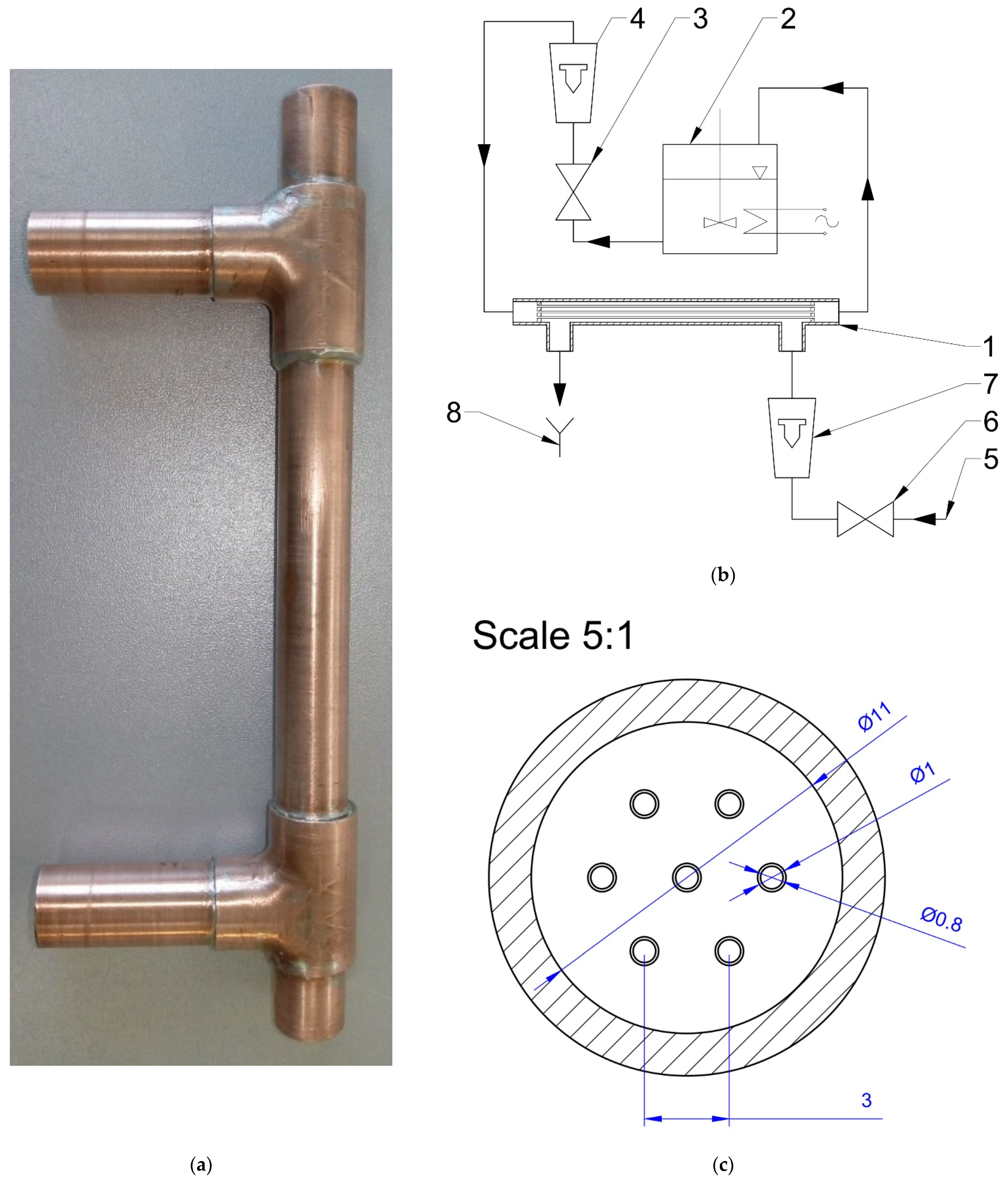
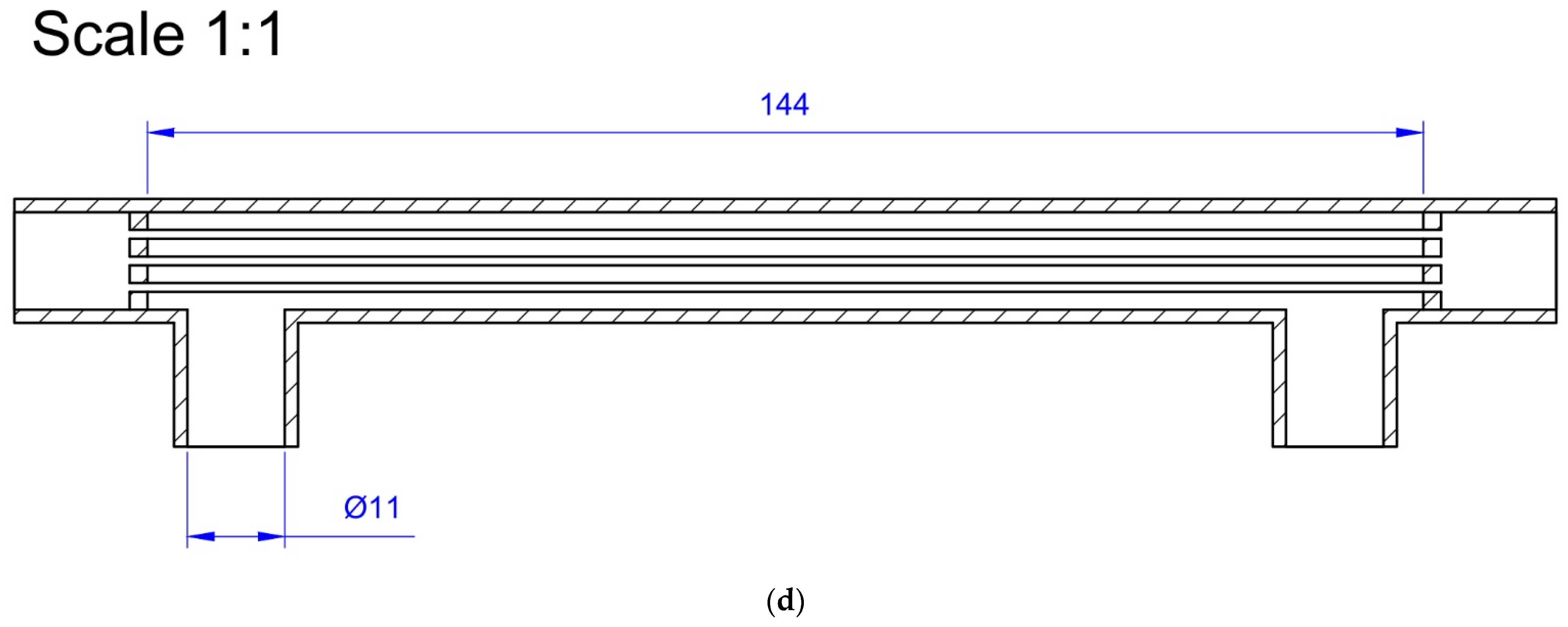
This paper presents the results of experimental tests performed using a shell and tube mini heat exchanger (STMHE). A schematic drawing of the analysed heat exchanger is shown in Figure 1. It consisted of seven brass tubes with outer diameter of , inner diameter of , and length of . The tubes were arranged in a hexagonal arrangement, and the tube pitch was equal to . The thermal conductivity coefficient of brass was assumed to be [20]. The tube sheet was made of thick copper sheet. The exchanger shell was made of copper and had an internal diameter equal to . All elements of the STMHE were connected by means of brazing. The heat exchanger was insulated along its entire length with an insulation layer made of polyurethane foam.
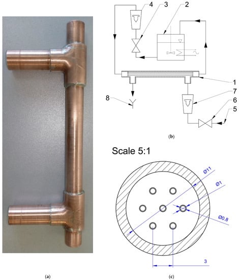
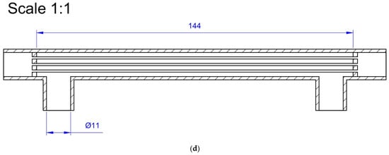
Figure 1.
(a) Investigated shell and tube mini heat exchanger (STMHE); (b) Experimental setup: 1—STMHE, 2—thermostatic vessel, 3—valve, 4—rotameter, 5—old water supply, 6—valve, 7—rotameter, 8—cold water drain; (c) cross section drawing of the investigated STMHE in 5:1 scale; (d) longitudinal section drawing of the investigated STMHE in 1:1 scale.
In the case of an industrial heat exchanger, the ratio of the outer diameter of the tubes to the pitch is usually in the range of . For the investigated STMHE, this ratio was larger than for macro heat exchangers and was equal to . Such a discrepancy was dictated by the difficulties in manufacturing a smaller size heat exchanger in the laboratory. However, it should be noted that the distance between the tube walls of the micro heat exchanger was smaller than for the macro heat exchangers. In addition, the values of pressure drop were significantly reduced due to the higher value of the ratio.
A schematic diagram of the STMHE is shown in Figure 1b. The mini heat exchanger (1) was operated in a water–water system. A thermostatic vessel (2) was used to control the temperature in the hot water circuit. The thermostat built–in pump was used to force the flow and the thermostat itself was filled with distilled water, which flowed in a closed circuit. The water flow rate was controlled by a valve (3) located on the line supplying liquid to the exchanger. The water flow rate was measured using a rotameter (4) mounted directly after the valve.
Cold water was supplied directly from the water network in an open circuit (5). The flow of cold water was regulated using a valve (6) and its flow rate was measured by a rotameter (7). The water flowing out of the STMHE was directed at a drain (8). The properties of distilled and tap water were measured at near ambient temperature. Density was determined using a calibrated pycnometer and viscosity with an Ubbelohde viscometer. The obtained values were not significantly different from the tabulated values. The physical properties of the water were therefore determined using the appropriate material tables for the average water temperature in the circuit. During experimental tests, the flow rate of hot water was varied in the range of , while that of cold water was varied in the range of . Taking into account the influence of temperature on the physical properties of the media, this resulted in superficial velocity in the range of and Reynolds number in the range of for hot water, and superficial velocity of and Reynolds number of for cold water.
The temperature of the media was measured at four points: the cold water inlet and outlet, and the hot water inlet and outlet. In this study, NTCLE101E3473SB0 [21] negative temperature coefficient (NTC) thermistors manufactured by Vishay were used to measure the temperature. The selected thermistors allow for temperature measurement with an accuracy of 0.5 °C without calibration, but can be calibrated to further reduce this value. All temperature sensors were placed in covers to separate them from the process media. The sensors were placed in close proximity to the fluid inlets and outlets, at a distance that ensured undisturbed fluid flow.
Temperature measurements were conducted using an Arduino Nano development board equipped with an ATmega328p microcontroller [22]. It features a 10-bit analog-to-digital converter (ADC) with successive approximation. The sampling frequency of the ADC was set to 38 kHz. Oversampling was used to increase the resolution of the ADC. The measurement was performed 64 times for each temperature sensor, thus increasing the effective number of bits to 13 [23], which resulted in temperature measurement resolution of . An NTC thermistor was connected in series with a precision resistor with a low temperature coefficient to form a voltage divider circuit. The resistor was located close to the microcontroller. The voltage divider was connected to supply voltage only during the measurement, otherwise both ends were connected to the ground. The resistance of the NTC thermistor was determined by measuring the voltage drop across the thermistor. The measurement procedure took 1.7 ms for each temperature sensor. To minimise the self–heating effect of the temperature sensor, the temperature measurement procedure was carried out at a frequency of 1 Hz, which is a sufficient frequency for steady-state measurements.
All temperature sensors were initially calibrated. The calibration consisted of immersing all sensors in water of known temperature and comparing their readings with those of a calibrated thermometer Termio–1 manufactured by Termoprodukt [24] which allows for temperature measurement with an accuracy of ±0.07 °C. The temperature ranges at the inlet and outlet of the media are shown in Table 1. The estimated uncertainty of indication of the calibrated NTC thermistors was ±0.20 °C and was confirmed by test runs.

Table 1.
Experimental temperature ranges.
The pressure drop during fluid flow was measured using a differential manometer. For the inter-pipe space its values ranged from . To measure the pressure drop, a differential manometer in the form of an inverted U-tube filled with water and a layer of air in its upper part was used. For the employed operating conditions, the pressure pulsations were small and the value of the pressure drop was stable, which allowed the differential pressure value to be determined with high accuracy and uncertainty of less than of the measured value. For the flow inside the tubes, the resulting pressure drop was in the range of . Due to the wide range of pressure drop values, two manometers were used for the measurement: for the pressure below , as in the case of the flow from the shell side, a U-tube manometer was used. For pressures above , a Capsuhelic 4000B–50KPA differential pressure gauge manufactured by Dwyer Instruments [25] was used, which allows for pressure measurement with an uncertainty of . This allowed relatively low measurement uncertainties over a wide range of process parameter values to be obtained.
2.2. Methods
2.2.1. Pressure Drop
For the pressure drop inside the tubes, the Darcy friction factor as a function of the velocity of the flowing medium was determined from the pressure drop measurements. It was calculated using the following transformed Darcy–Weisbach equation in Equation (1) [26]:
where is the Darcy friction factor, is the internal diameter of the pipe, is the pressure drop, is the pipe length, is the density of the fluid, and is the fluid velocity.
If minor losses are considered in addition to frictional losses, the above equation takes the form of Equation (2) [26]:
where is the minor loss coefficient.
In the considered case, the minor losses are related to minor losses at the inlet and the outlet of the pipeline characterised by sharp edges. The value of the minor loss coefficients for these cases are and , respectively, which adds up to [26].
In order to validate the obtained results, they were compared with correlations available in the literature for determining the Darcy friction factor. Because it was not possible to determine the surface roughness coefficient of the tubes, the correlations that do not account for roughness coefficient or surface roughness were mainly used, or the roughness was assumed to be zero. The correlations used to determine the value of the drag coefficient are usually functions of the Reynolds number [27], defined as Equation (3):
where is the viscosity of fluid.
The following correlations were used for the calculations of :
- (a)
- The correlation for laminar fluid flow [26] (Equation (4)):
- (b)
- Blasius [28] correlation (Equation (5)):
- (c)
- Filonenko [29] correlation (Equation (6)):
- (d)
- Haaland [30] correlation (Equation (7)):
- (e)
- McAdams [31] correlation (Equation (8)):
For the flow on the shell side, the ratio of length to flow diameter is much smaller than in the case of flow through the pipe. Therefore, the major source of flow pressure drop here will be minor loses; thus, a slightly different methodology was adopted in the calculations. Instead of determining the Darcy friction factor, it was decided to determine the minor loss coefficient. The equation for laminar flow (Equation (4)) was used to calculate the Darcy friction factor for , whereas for the Blasius equation of Equation (5) was used. The value of the minor loss coefficient was then determined using the following transformed Darcy–Weisbach equation (Equation (9)) [26]:
where is the equivalent diameter, which can be calculated for the flow parallel to the tube bundle according to Equation (10):
As used previously, the equivalent diameter was used as the characteristic length to determine the Reynolds number, i.e., Equation (3).
2.2.2. Overall Heat Transfer, Shell and Tube Side Convective Heat Transfer
The aim of this study was to determine the value of the overall heat transfer coefficient depending on the process parameters. The value of was determined based on media temperatures at their inlets or outlets, and their flow rates. The first step in determining the overall heat transfer coefficient consisted in determination of the amount of heat given off by the hot medium (Equation (11)) and the amount of heat received by the cold medium (Equation (12)):
where is the thermal power in , is the volumetric flow rate in , is the specific heat in , is the temperature in . Subscripts and denote hot and cold fluid, respectively, whereas subscripts and denote inlet and outlet conditions, respectively.
The calculated thermal output for the hot fluid and the cold fluid should agree. Because the hot water flow rate was much smaller than the cold water flow rate, the temperature difference between the cold water inlet and outlet was much smaller than for the hot water. The temperature difference for hot water was in the range of , whereas that for cold water was in the range of . This means that in some cases the measurement uncertainty of the temperature difference was larger than the determined value of the temperature difference itself. For this reason, instead of using the arithmetic mean of and to calculate the amount of exchanged heat, only the value of heat given off by the hot medium was used. The temperature of the hot fluid was measured in the direct vicinity of the inlet and outlet to the heat exchanger tubes, and the heat exchanger itself was well insulated, so the heat loss in the space before and after the heat exchanger tubes was negligibly small. In addition, the hot medium was located in the inner part of the exchanger, which additionally reduced the potential heat losses. Knowing the amount of heat exchanged, the temperatures of the media, and the geometry of the heat exchanger, the value of the overall heat transfer coefficient can be calculated as Equation (13):
where is the overall heat transfer coefficient, is the heat transfer area, and is the logarithmic mean temperature difference, which for the counter current flow can be calculated as Equation (14):
Based on the inner surface area of the tubes, the overall heat transfer coefficient can be calculated as Equation (15):
where is the convective heat transfer coefficient and is the tube material heat conductivity. In the above formula, subscripts and denote the shell and tube side, respectively.
The experimentally derived convective heat transfer coefficients were compared with those calculated from the correlations available in the literature.
The heat transfer coefficients were determined from the value of the dimensionless Nusselt number Nu [32], defined as Equation (16):
For the flow inside the tubes, the diameter in Equation (16) is the inner diameter of the tubes . Many different correlations for the value of the Nusselt number can be found in the literature. Such correlations are usually a function of the dimensionless Reynolds number , and Prandtl number [31], which can be defined as Equation (17):
To describe the heat transfer inside circular tubes, we can use, among others, Shah’s [33] correlation for laminar flow (Equation (18)):
Another relation applying to laminar flow is that proposed by Sieder and Tate (Equation (19)) [34]:
where is the water viscosity at the mean fluid temperature.
For the turbulent flow, Sieder and Tate [34] proposed the correlation in Equation (20):
Dittus and Boelter [35] suggested a similar correlation, which can be expressed as in Equation (21):
Gnielinski developed two correlations [36], given by Equations (22) and (23), both applying to transition flow and fully developed turbulent flow:
where can be calculated using the Filonenko correlation of Equation (6) [29].
For the transition and developing turbulent flow, Hausen [37] suggested using the correlation in Equation (24):
Recently, Ünverdi and co-workers [13] proposed two correlations, for transition (Equation (25)) and turbulent flow (Equation (26)) in minichannels, that is:
For the shell side flow, and dimensionless numbers are calculated using the equivalent diameter as the characteristic length. The correlations used to calculate on the tube side usually yield erroneous values. For this reason, different types of correlations are used for calculating at the shell side. Nitsche [38] suggested using two types of correlations, one for a square tube arrangement (Equation (27)) and the second one for a triangular tube arrangement (Equation (28)):
For the shell side calculation, the McAdams [31] correlation of Equation (29) can also be used:
Kücük and co-workers [27] developed the correlation in Equation (30):
For flow parallel to the tube bundle, Weismann [39] suggests using the correlation in Equation (31) for hexagonal tube arrangement:
where is the tube pitch (distance between two adjacent tubes axis).
For the shell and tubes heat exchangers without baffles, Kozioł [40] suggests using the empirical equation of Equation (32):
2.2.3. Determination of the Heat Transfer Coefficients
Determining the convective heat transfer coefficient is a complex and often problematic task. Convective heat transfer is the heat exchange between a wall and a fluid flowing in direct contact with the wall. The driving force of this process is the temperature difference between the wall and the fluid bulk. Therefore, to determine its value, in addition to the mentioned heat output, it is necessary to know the temperature of the wall and the fluid. In the case of heat transfer in micro- and minichannels, measuring the wall temperature is difficult, because even the smallest temperature sensors often have dimensions comparable to or even larger than the diameter of such a channel.
One method of determining the channel wall temperature is to form channels on one surface of a block made of a metal having a high thermal conductivity coefficient. Such a block is heated on one side by a heating element of known thermal power. On the other side, the block is cooled by the flowing fluid. If the side walls are insulated, the process reduces to one–dimensional heat conduction. Thus, knowing the temperature gradient inside the block and the temperature at a certain distance from the microchannels, we can calculate the temperature prevailing on the surface of the microchannels walls.
Unfortunately, this methodology can only be used for heat transfer in micro- and minichannels and cannot be applied to heat exchangers. In this case, it is common practice to calculate the heat transfer coefficient using the experimentally determined overall heat transfer coefficient. For one of the exchanger passes, the heat transfer coefficient is determined using commonly available literature correlations. The second heat transfer coefficient is determined from the definition of the overall heat transfer coefficient (Equation (15)). To further reduce possible errors, the operating parameters of the exchanger in the circuit, for which the heat transfer coefficient is calculated from the literature correlation, are kept constant so that the value of the heat transfer coefficient is approximately constant for all experiments performed.
Unfortunately, the methods mentioned above have limited use or require certain assumptions to be made. If the value of the heat transfer coefficient in the assumed heat exchanger circuit deviates from the one determined by the selected empirical correlation, this can contribute to the introduction of a systematic error, often of significant value. In this study, however, a different methodology was used. In order to determine the correlations for calculating the heat transfer coefficients, the appropriate forms of correlation equations were first adopted. It was assumed that for the range of Reynolds number for the flow inside the tubes (), we can deal with laminar flow (for small values of ) and turbulent flow. For each of these ranges, a separate form of correlation for the Nusselt number was adopted. It was assumed that the change in the flow type occurs when the critical value of the Reynolds number is exceeded. For laminar flow, it is assumed that the Nusselt number can be calculated using the equation in the general form of Equation (33):
For turbulent flow, the form of Equation (34) was adopted:
For the flow on the shell side, only one type of flow was assumed and therefore only one form of correlation for Nusselt number, as in Equation (35):
The obtained correlation equations can then be used to determine the heat transfer coefficients for the flow in tubes () and in the exchanger shell () using Equation (16). For flow in tubes, the inner diameter of the tubes was taken as the diameter in the equations for calculating the Reynolds number (Equation (3)) and Nusselt number (Equation (16)), whereas for flow in the exchanger shell, the equivalent diameter was adopted to determine Re and Nu. The calculated heat transfer coefficients can in turn be used to determine the overall heat transfer coefficient according to Equation (15). Thus, it can be concluded that for certain values of Reynolds and Prandtl numbers for the fluid flowing in the tubes and shell space, the value of the calculated heat transfer coefficient is a function of eleven variables, which are the coefficients of Equations (33)–(35) and the value of the critical Reynolds number , which can be expressed as in Equation (36):
Determining the values of the coefficients of Equation (36) therefore reduces to an optimisation problem. To resolve this problem, the objective function of Equation (37) was defined:
where is the number of conducted experiments.
The effects of flow velocity and media temperature were investigated during the experiments. The studied range of variation in these parameters translated into Reynolds number values for the flow in tubes in the range , and for the flow in the shell of , whereas the value of Prandtl number varied in the range for the flow in tubes, and for the flow in the shell. The range of variation of Prandtl number values was relatively small, both for the flow in the tubes and for the flow in the shell. For this reason, it was decided to assume that their values were constant and equal, as shown in Equation (38):
This value appears most frequently in the correlation equations available in the literature (see Equations (18)–(20) and (24)–(31)). The objective function of Equation (37) therefore reduces to the form of Equation (39):
As a result of this assumption it was possible to reduce the number of searched variables to eight instead of eleven, which significantly simplified the computational procedure. The procedure for the determination of coefficients was based on the search for the global minimum of Equation (39). The optimisation procedure was carried out according to the following algorithm:
- (1)
- Initial assumption of the values of coefficients in Equation (39) and determination of the range of variation in these parameters.
- (2)
- Calculation of the values of Nusselt numbers for the tube and shell side flow based on experimental values of Reynolds and Prandtl numbers using Equations (33)–(35).
- (3)
- Calculation of the values of heat transfer coefficients based on Equation (16) and of the overall heat transfer coefficient using Equation (15).
- (4)
- Calculation of the value of the objective function using Equation (39).
- (5)
- Correcting the values of coefficients until the minimum of the function defined by Equation (39) is reached.
MATLAB 2018b software was used to carry out the calculations. To determine the optimal values of the sought parameters, the built–in fmincon function [41] was used, which allows determination of the minimum of a function of multiple variables with constraints. Calculations were performed using the interior–point algorithm and default tolerance values (constraint tolerance and optimality tolerance equal to , step tolerance and absolute tolerance for the projected conjugate gradient algorithm equal to ) [41]. The lower and upper bounds of the coefficients were estimated on the basis of the values of these parameters in the classical equations available in the literature (e.g., see Equations (18)–(32)). In order to ensure that the coefficients were determined correctly, the lower and upper bounds were selected so that the calculated parameters were not located at the boundary, but inside it. The bounds values of the coefficients are shown in Table 2.
Table 2.
Lower and upper bounds of coefficients.
The values of the determined coefficients were related to the initial values of these parameters. Equation (39) is a non-linear relation that additionally incorporates experimental measurements subject to some measurement uncertainty. Therefore, the optimised function therefore has multiple local minima. In order to determine the value of the global minimum of Equation (39), the numerical procedure described above was carried out repeatedly using random initial values of the optimisation parameters.
3. Results and Discussion
3.1. Tube Side Pressure Drop
The experimental values of the Darcy friction factor without the influence of the inlet and outlet minor loss coefficients were calculated according to Equation (1), and then accounting for the influence of the tubes inlet and outlet using Equation (2).
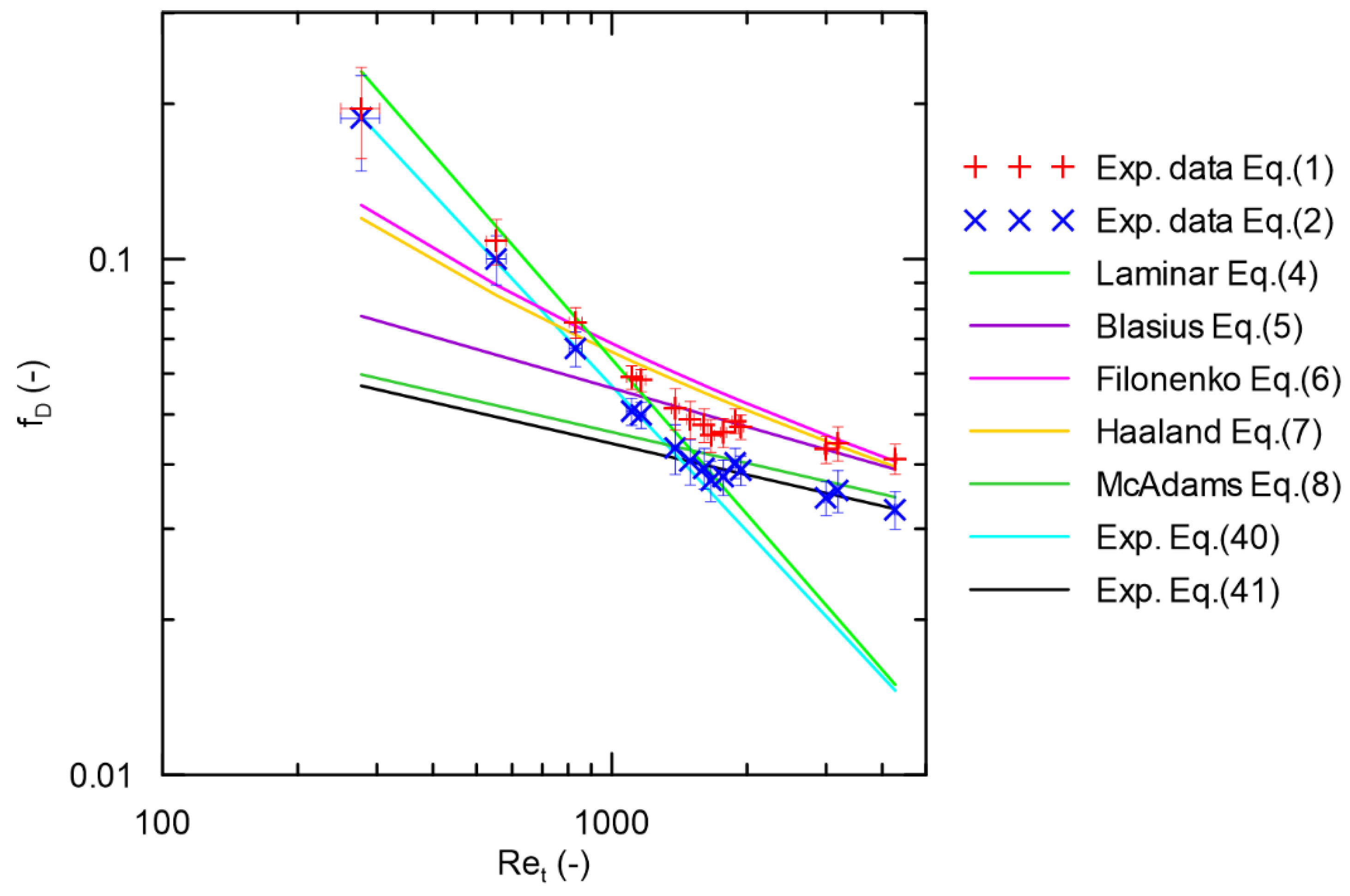
Figure 2 shows the experimental values of the Darcy friction factors. The values calculated using Equations (4)–(8) are also presented. The figure clearly shows that we can divide the values of the friction factors calculated using the literature correlations into two groups: correlation for laminar flow (Equation (4)) and correlations for turbulent flow (Equations (5)–(8)), which obviously coincides with the range of applicability of the analysed correlations given by the authors. We can note that the correlations of Filonenko [29] and Haaland [30], i.e., those given by Equations (6) and (7), respectively, give practically identical results for the entire range of Reynolds number values studied (). For , the Blasius [28] correlation (Equation (4)) also gives very similar results to those obtained using the correlations proposed by Filonenko and by Haaland. Finally, the McAdams [31] correlation (Equation (8)) asymptotically approaches the results obtained from other correlations in the turbulent flow regime. The value of pipe surface roughness was not taken into account when calculating the friction coefficient, so similar results for turbulent flow are not surprising.
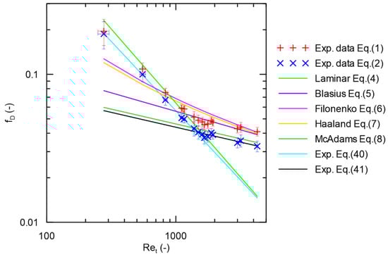
Figure 2.
Darcy friction factor on the tube side flow as a function of the Reynolds number.
Comparing the experimental results with those obtained from literature correlations we can observe that for small values of Reynolds number the determined friction factors correlate very well with Equation (4) for laminar flow. When a certain critical value of the Reynolds number is exceeded a qualitative change in the obtained experimental results can be observed. Such a change is due to the change in the type of flow that occurs in the tubes from laminar to transitional (turbulent). For flow through a macro-tube with a circular cross-section, the value of the critical Reynolds number is usually adopted as the conventional threshold for this transition. However, as reported in the literature, for tubes with a diameter smaller than 1 mm, such a transition can occur earlier than in tubes with a larger diameter. From Figure 2 we can conclude that such a transition occurs here for Reynolds number values in the range of . The Darcy friction factor for the studied STMHE with respect to minor losses can be approximated by power law correlations for , as in Equation (40):
and for , as in Equation (41):
3.2. Shell Side Pressure Drop
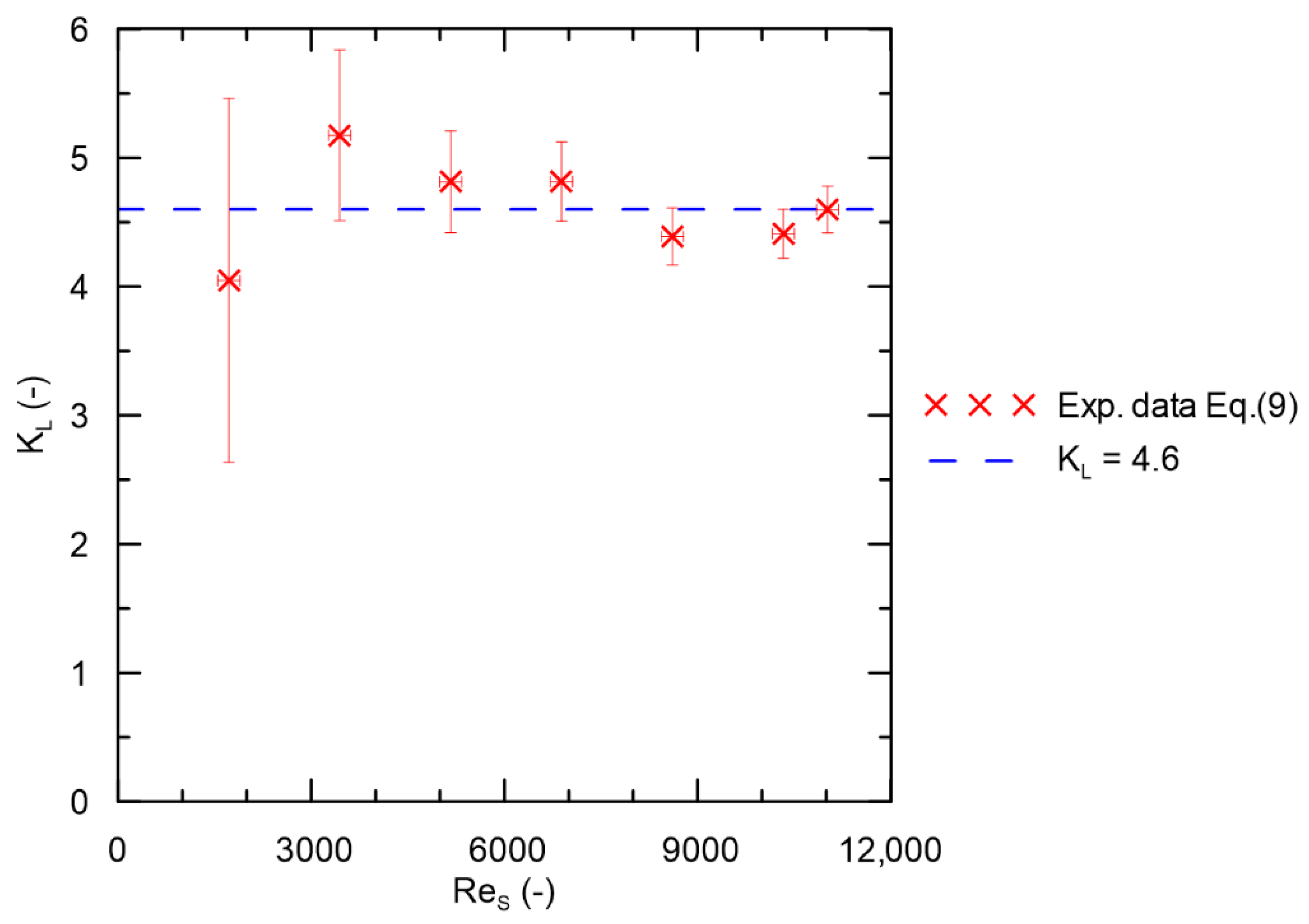
For flow in the shell side the minor loss coefficients were determined according to Equation (9). For turbulent flow in ducts of complex shape it is usually assumed that the coefficients of frictional resistance are determined from classical correlations for circular ducts; however, when calculating the Reynolds number, the equivalent diameter is taken as the diameter of the duct, and the same was done in this case. For turbulent flow in a hydraulically smooth pipe, the values of the Darcy friction factor calculated using different correlations practically do not differ significantly from each other. For this reason, to simplify the calculations, it was assumed that the Darcy friction factor can be determined using the Blasius equation of Equation (5) [28]. The results of the calculations are shown in Figure 3. It can be seen that, after taking into account the measurement uncertainties, the value of the local resistance coefficient is practically constant and is, on average, . However, it should be noted that the determined minor loss coefficient includes four components: the change in flow direction at the inlet to the shell side, the spreading of the liquid stream between the tubes, the recombination of smaller streams into one larger one, and the second sudden change in flow direction at the outlet of the shell side.
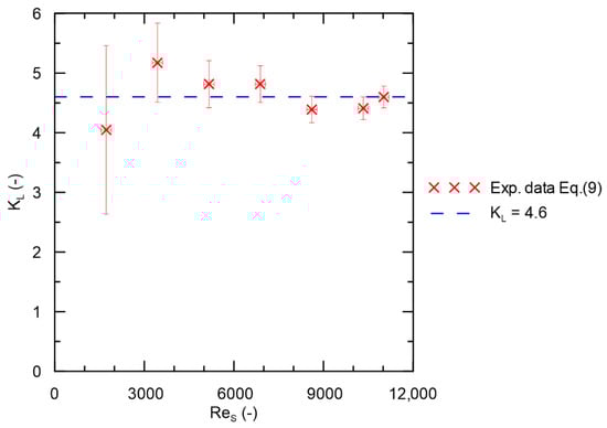
Figure 3.
Minor loss coefficient on the shell side as a function of the Reynolds number.
3.3. Convective Heat Transfer Coefficient
The optimisation procedure carried out allowed the critical value of the Reynolds number to be obtained, which was found to be equal to . The correlations for the calculation of the value of Nusselt numbers in general form given by Equations (33)–(35) can be thus written in the form of the Equations (42)–(44):
In order to validate the correlations obtained, they were compared with those available in the literature. For this purpose, the values of heat transfer coefficients calculated using the literature correlations (Equations (18)–(32)) and the obtained experimental correlations (Equations (42)–(44)) were determined. The results of the comparison are presented in Figure 4, Figure 5 and Figure 6.
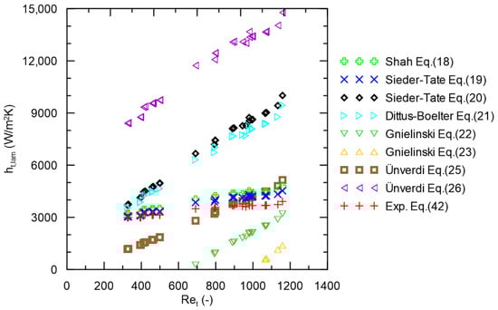
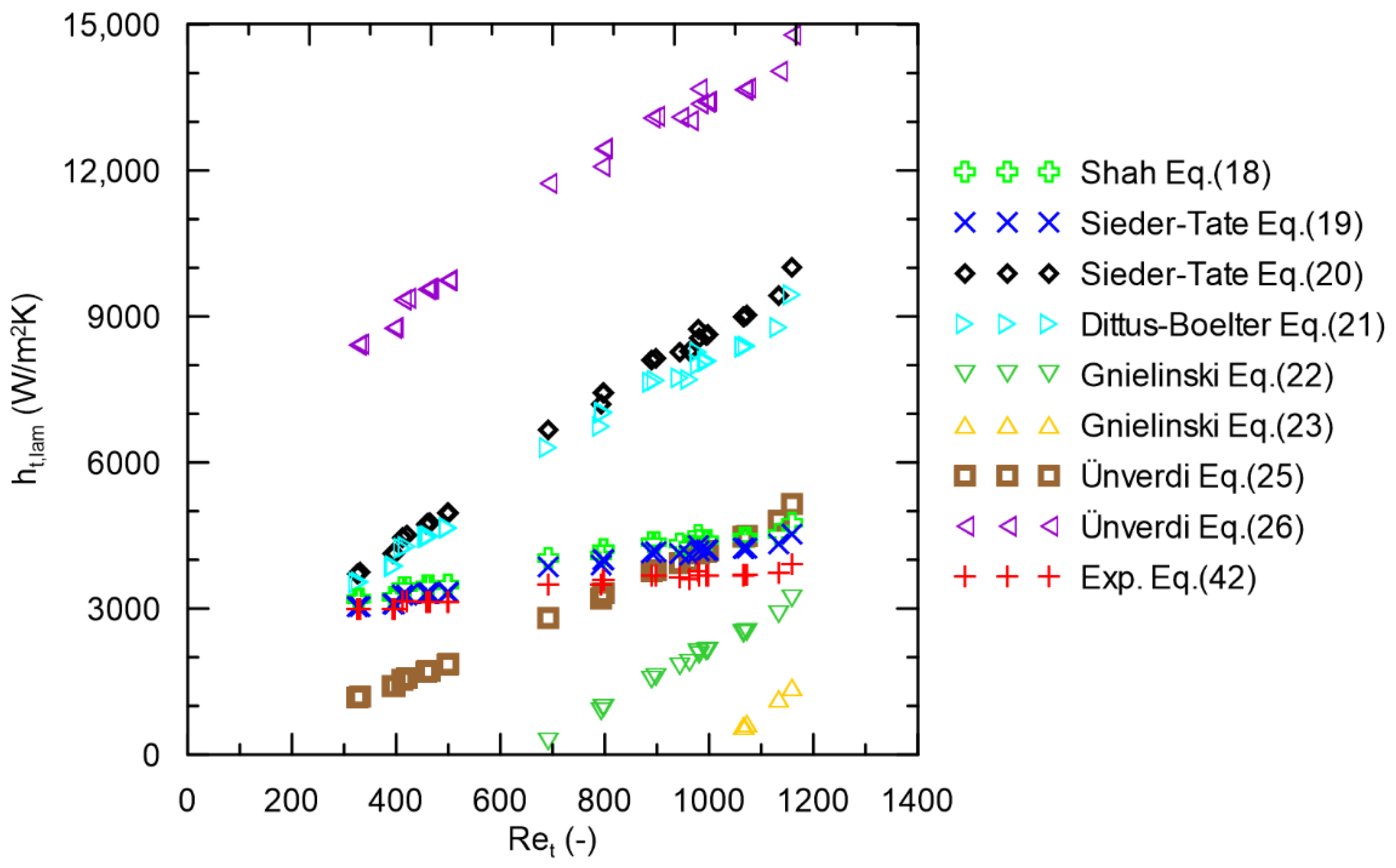
Figure 4.
Heat transfer coefficient for the laminar flow inside tubes as a function of the tube side Reynolds number .
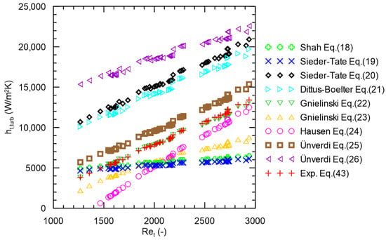
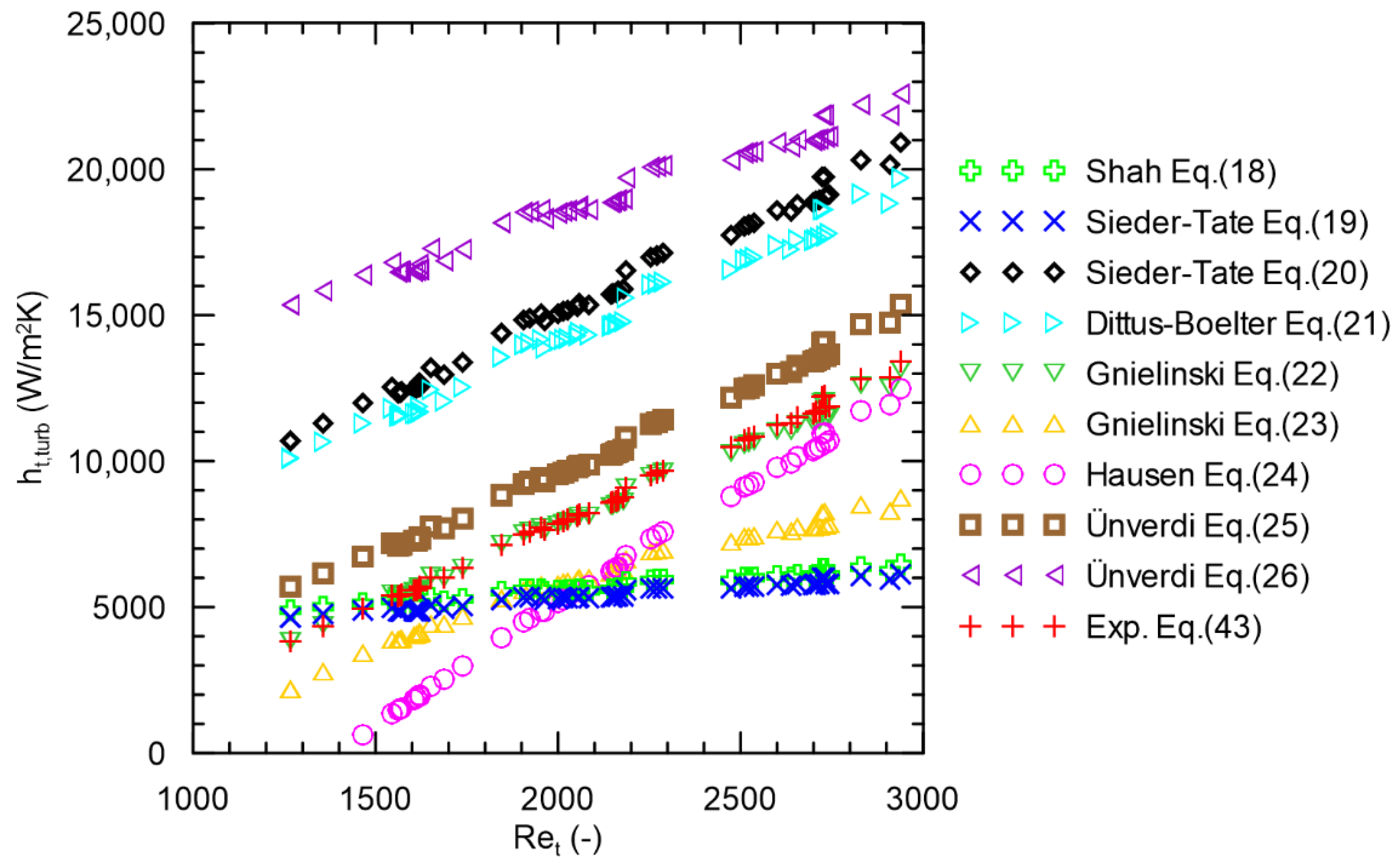
Figure 5.
Heat transfer coefficient for the transition or turbulent flow inside tubes as a function of the tube side Reynolds number .
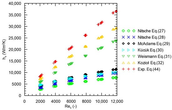
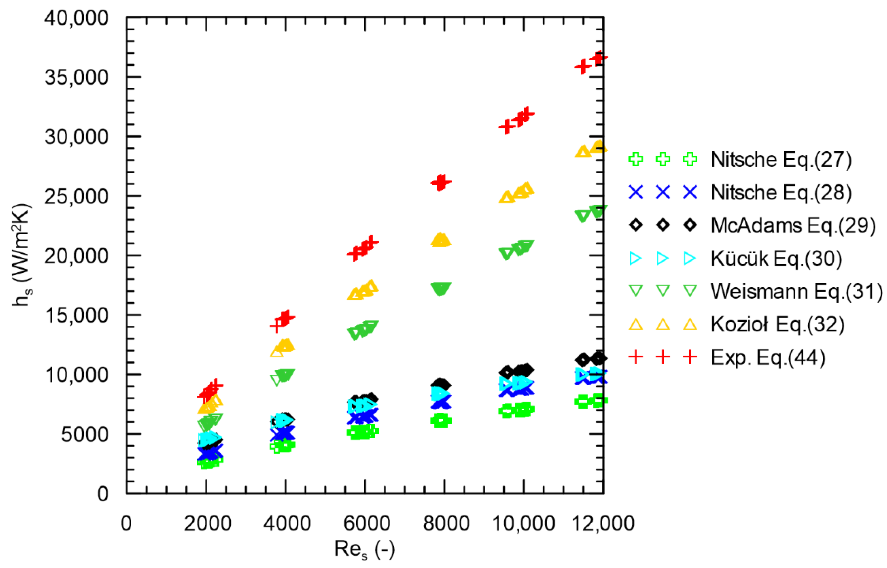
Figure 6.
Heat transfer coefficient for the flow at the shell side as a function of the Reynolds number .
Figure 4 shows the dependence of the heat transfer coefficient from the tube side on the Reynolds number for laminar flow. The figure compares the experimentally obtained correlation of Equation (42) with all the correlations for tube flow, both for laminar (Equations (18) and (19)) and turbulent (Equations (20)–(26)) flow. It can be seen that the slope of the calculated heat transfer coefficients for turbulent flow is much steeper than that for the correlations for laminar flow. The experimental results most closely match those obtained from the Sieder–Tate correlation for laminar flow (Equation (19)); however, it gives slightly underestimated results compared to the correlation of Equation (42).
Figure 5 shows the results for turbulent fluid flow through the exchanger tubes. As in the case of laminar flow, all correlations for the flow inside the tubes (Equations (18)–(26)) are presented and compared with the correlation proposed in this work (Equation (43)). We can see here that, in this case, the correlations for turbulent flow (Equations (20)–(26)) describes a qualitative variation of the heat transfer coefficient. The best fit to the results obtained using the experimental correlation (Equation (43)) is obtained from Equation (22) proposed by Gnielinski for transitional and turbulent flow. In this case, practically identical results were obtained as for the experimental correlation formulated here. The correlation proposed by Ünwerdi and co-workers has a similar qualitative agreement but gives results about higher than compared to Equation (43).
The values of the heat transfer coefficient for the shell side determined using the experimental correlation (Equation (44)) and correlation Equations (27)–(32) are presented in Figure 6. The best agreement of the results obtained using the experimental correlation (Equation (44)) is obtained from Equation (32), which was proposed by Kozioł. It can be observed here that the correlations of Equations (27)–(30) allow similar values of the heat transfer coefficient to be obtained. The mentioned correlations were derived for heat exchangers with baffles. For these correlations, the definition of the Reynolds number is not related to the cross-sectional flow area of the heat exchanger, but to the flow area across the heat exchanger tubes between the baffles. For this reason, these correlations cannot be applied to heat exchangers without baffles, such as the heat exchanger under study. Correlations of Equations (31) and (32) were proposed for the flow along the group of tubes in a heat exchanger without baffles; hence, a much better match was achieved with the experimental correlation. The correlation proposed by Weismann (Equation (31)) was derived for the case of flow along a bundle of tubes with no change in flow direction at the inlet to the outlet of the exchanger. The correlation by Kozioł in Equation (32), in contrast, was derived for the case of flow along a bundle of pipes taking into account the change in direction at the exchanger inlet and outlet. This situation corresponds more closely to the heat exchanger investigated in this study, which is also reflected in a better fit to the experimental correlation of Equation (44). However, it should be noted that the equation proposed by Kozioł has a different range of applicability ( as the one presented in this paper (; ; in this study), which could be the reason for the differences seen in Figure 6.
The experiments performed did not allow experimental values of heat transfer coefficients to be determined, so we cannot directly compare the experimental and calculated values of heat transfer coefficients. However, it is possible to determine the overall heat transfer coefficient values and compare them with the experimental values. Such a comparison is shown in Figure 7. There are two series of data: one represents the overall heat transfer coefficient calculated using the correlations determined experimentally in this study (Equations (42)–(44)), whereas the other represents the results obtained using the literature correlations for which the determined values of heat transfer coefficients match best to the results determined using the experimental correlations determined in this work (Equations (42)–(44)), i.e., the Sieder–Tate correlation for laminar flow inside pipes (Equation (19)), the Gnielinski correlation for transitional and turbulent flow inside pipes (Equation (22)), and the Kozioł correlation for flow along a pipe bundle (Equation (32)). The solid line indicates the diagonal of the diagram, i.e., the zone where the calculated results perfectly coincide with the experimental results. The dashed lines indicate the ±10% deviation from the diagonal. Taking into account the measurement uncertainties, we can see that in both cases a good agreement between the calculated results and the experimental results was achieved. Most of the calculated results do not deviate from the experimental results by more than 10%.
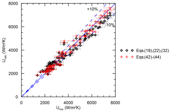
Figure 7.
Comparison of experimentally obtained overall heat transfer coefficients with the values calculated using: (a) Sieder–Tate (Equation (19)), Gnielinski (Equation (22)), and Kozioł (Equation (32)) correlations; (b) correlations derived in this study (Equations (42)–(44)).
4. Conclusions
This paper presents the results of experimental studies aimed at determination of the heat transfer coefficient and pressure drop, both inside the tubes and in the shell side of the mini heat exchanger. The empirical formulas describing the values of the Nusselt number depending on the values of dimensionless Reynolds and Prandtl numbers were formulated. A new method based on optimisation was used to determine parameters present in the equations. The results were also compared with correlation equations available in the literature.
Examination of the pressure drop values during flow in the exchanger tubes allowed the Darcy friction coefficients to be determined. The determined values of friction coefficients qualitatively changed their tendency after exceeding a certain critical value of the Reynolds number. Below this value, the friction coefficients were best represented by the correlation of Equation (4), which was determined theoretically for laminar flow through a tube with a circular cross-section. For flow above the critical value of the Reynolds number, the best representation of experimentally determined values of the friction coefficients was obtained from Equation (5) proposed by Blasius.
For the shell side, the sources of pressure drop were mainly minor losses resulting from the change in flow direction at the inlet and outlet of the exchanger, and from the change in flow direction during inflow and outflow from the inter–tube space. The experiments allowed determination of the resultant value of the local resistance coefficients for the cases given as equal to .
The heat transfer coefficients were determined using an original optimisation–based method proposed in this work. The method allowed the simultaneous determination of correlations for the Nusselt number for both tube flow and flow through the shell side. The determination of coefficients of experimental correlation for the Nusselt number did not require the knowledge of the heat exchanger wall temperature value nor the assumption of a correlation describing heat transport in one of the exchanger circuits.
Investigations of the heat exchange inside the heat exchanger tubes confirmed the change in flow type from laminar to transitional, and allowed determination of the critical Reynolds number, which was found to be . This value is consistent with the observations made during the analysis of fluid pressure drop during flow through the tubes.
The conducted research allowed determination of the correlation equations for the investigated heat exchanger (Equations (42)–(44)). The analysis of the correlations available in the literature made it possible to find equations which allowed the derivation of often practically identical values of the calculated heat transfer coefficient as for the correlations determined in this study.
The correlations taken from the literature often had a slightly different form from the equations determined on the basis of experimental results presented in this paper; however, the results obtained using them were found to be consistent with the correlations of Equations (42)–(44). The discrepancies shown may result from the fact that the selected literature correlations were usually derived for a much wider range of heat exchanger operating parameters, and therefore they represent a better generalisation of the variation of heat transfer coefficients as a function of apparatus operating conditions. Moreover, the applicability limits proposed by the authors often did not coincide with the experimental ones; however, they still satisfactorily reproduced the values of heat transfer coefficients, which confirms that the selected literature correlations provide a very good generalisation of heat transfer. Finding equivalents in the literature further confirms the validity of the method used to determine the heat transfer coefficients based on optimisation.
Author Contributions
Conceptualization, M.P.; methodology, M.P.; software, M.P.; validation, M.P.; formal analysis, M.P. and A.K.; investigation, M.P. and A.K.; resources, M.P.; data curation, M.P.; writing—original draft preparation, M.P.; writing—review and editing, M.P.; visualization, M.P.; supervision, M.P.; project administration, M.P.; funding acquisition, M.P. All authors have read and agreed to the published version of the manuscript.
Funding
This research received no external funding.
Institutional Review Board Statement
Not applicable.
Informed Consent Statement
Not applicable.
Data Availability Statement
The data presented in this study are available on request from the corresponding author.
Conflicts of Interest
The authors declare no conflict of interest.
References
- Wu, P.; Little, W.A. Measurement of the heat transfer characteristics of gas flow in fine channel heat exchangers used for microminiature refrigerators. Cryogenics 1984, 24, 415–420. [Google Scholar] [CrossRef]
- Morini, G.L. Single–phase convective heat transfer in microchannels: A review of experimental results. Int. J. Therm. Sci. 2004, 43, 631–651. [Google Scholar] [CrossRef]
- Mehendale, S.S.; Jacobi, A.M.; Shah, R.K. Fluid flow and heat transfer at micro–and meso–scales with application to heat exchanger design. Appl. Mech. Rev. 2000, 53, 175–193. [Google Scholar] [CrossRef]
- Kandlikar, S.G.; Grande, W.J. Evolution of microchannel flow passages––thermohydraulic performance and fabrication technology. Heat Transf. Eng. 2003, 24, 3–17. [Google Scholar] [CrossRef]
- Al–Janabi, R.; Coletti, F.; Mahmoud, M.M.; Karayiannis, T.G. Experimental Study of Flow Boiling Using R134a in Multi Microchannels. In Proceedings of the 5th World Congress on Mechanical, Chemical, and Material Engineering (MCM’19), Lisbon, Portugal, 15–17 August 2019. Paper No. HTFF 133. [Google Scholar] [CrossRef]
- Kee, R.J.; Almand, B.B.; Blasi, J.M.; Rosen, B.L.; Hartmann, M.; Sullivan, N.P.; Zhu, H.; Manerbino, A.R.; Menzer, S.; Coors, W.G.; et al. The design, fabrication, and evaluation of a ceramic counter–flow microchannel heat exchanger. Appl. Therm. Eng. 2011, 31, 2004–2012. [Google Scholar] [CrossRef]
- Cao, H.; Chen, G.; Yuan, Q. Testing and design of a microchannel heat exchanger with multiple plates. Ind. Eng. Chem. Res. 2009, 48, 4535–4541. [Google Scholar] [CrossRef]
- Wang, Q.; Dai, C. Experimental study on heat transfer and pressure drop of micro–sized tube heat exchanger. Trans. Tianjin Univ. 2014, 20, 21–26. [Google Scholar] [CrossRef]
- Hejcik, J.; Jicha, M. Single phase heat transfer in minichannels. EPJ Web Conf. 2014, 67, 2034. [Google Scholar] [CrossRef] [Green Version]
- Col, D.D.; Cavallini, A.; Da Riva, E.; Mancin, S.; Censi, G. Shell–and–tube minichannel condenser for low refrigerant charge. Heat Transf. Eng. 2010, 31, 509–517. [Google Scholar] [CrossRef]
- Yan, Y.Y.; Lin, T.F. Condensation heat transfer and pressure drop of refrigerant R–134a in a small pipe. Int. J. Heat Mass Tran. 1999, 42, 697–708. [Google Scholar] [CrossRef]
- Adams, T.M.; Abdel–Khalik, S.I.; Jeter, S.M.; Qureshi, Z.H. An experimental investigation of single–phase forced convection in microchannels. Int. J. Heat Mass Tran. 1998, 41, 851–857. [Google Scholar] [CrossRef]
- Ünverdi, M.; Kücük, H.; Yılmaz, M.S. Experimental investigation of heat transfer and pressure drop in a mini–channel shell and tube heat exchanger. Heat Mass Tran. 2019, 55, 1271–1286. [Google Scholar] [CrossRef]
- Kücük, H.; Ünverdi, M.; Yılmaz, M.S. Experimental investigation of shell side heat transfer and pressure drop in a mini–channel shell and tube heat exchanger. Int. J. Heat Mass Tran. 2019, 143, 118493. [Google Scholar] [CrossRef]
- Rajalingam, A.; Chakraborty, S. Effect of shape and arrangement of micro–structures in a microchannel heat sink on the thermo–hydraulic performance. Appl. Therm. Eng. 2021, 190, 116755. [Google Scholar] [CrossRef]
- Ahmed, H.E.; Kherbeet, A.S.; Ahmed, M.I.; Salman, B.H. Heat transfer enhancement of micro–scale backward-facing step channel by using turbulators. Int. J. Heat Mass Tran. 2018, 126, 963–973. [Google Scholar] [CrossRef]
- Zhuang, D.; Yang, Y.; Ding, G.; Du, X.; Hu, Z. Optimization of microchannel heat sink with rhombus fractal-like units for electronic chip cooling. Int. J. Refrig. 2020, 116, 108–118. [Google Scholar] [CrossRef]
- Jung, S.Y.; Park, H. Experimental investigation of heat transfer of Al2O3 nanofluid in a microchannel heat sink. Int. J. Heat Mass Tran. 2021, 179, 121729. [Google Scholar] [CrossRef]
- Ekiciler, R.; Arslan, K. CuO/water nanofluid flow over microscale backward-facing step and analysis of heat transfer performance. Heat Tran. Res. 2018, 49, 1489–1505. [Google Scholar] [CrossRef]
- Engineering Thermal Properties of Metals, Conductivity, Thermal Expansion, Specific Heat—Engineers Edge. Available online: https://www.engineersedge.com/properties_of_metals.htm (accessed on 29 November 2021).
- Vishay–NTC Thermistors, Radial Leaded Special Accuracy. Available online: https://www.vishay.com/docs/29046/ntcls101.pdf (accessed on 30 November 2021).
- Atmel ATmega328P Datasheet. Available online: https://ww1.microchip.com/downloads/en/DeviceDoc/Atmel–7810–Automotive–Microcontrollers–ATmega328P_Datasheet.pdf (accessed on 29 November 2021).
- AN118–Improving ADC Resolution by Oversampling and Averaging. Available online: https://www.cypress.com/file/236481/download (accessed on 30 November 2021).
- Pharmacy Vaccine Low Temperature Data Logger Termio–1. Available online: https://termoprodukt.co.uk/industrial–fridge–temperature–external–sensor–data–recorder–termio–1 (accessed on 9 November 2021).
- Dwyer—Series 4000 CAPSUHELIC® Differential Pressure Gage. Available online: https://www.dwyer–inst.com/Product/Pressure/DifferentialPressure/Gages/Series4000 (accessed on 29 November 2021).
- White, F.M. Fluid Mechanics, 7th ed.; McGraw–Hill: New York, NY, USA, 2011. [Google Scholar]
- Reynolds, O. On the dynamical theory of incompressible viscous fluids and the determination of the criterion. Philos. Trans. R. Soc. Lond. 1895, 186, 123–164. [Google Scholar] [CrossRef]
- Blasius, H. Boundary Layers in Liquids with Low Friction. Z. Math. Phys. 1908, 56, 1–37. (In German) [Google Scholar]
- Filonenko, G.K. Hydraulic resistance in pipes. Teploenergetika 1954, 1, 40–44. (In Russian) [Google Scholar]
- Haaland, S.E. Simple and Explicit Formulas for the Friction Factor in Turbulent Pipe Flow. J. Fluids Eng. 1983, 105, 89–90. [Google Scholar] [CrossRef]
- McAdams, W.H. Heat Transmission, 3rd ed.; McGraw–Hill: New York, NY, USA, 1954. [Google Scholar]
- Nusselt, W. The dependence of the heat transfer coefficient on tube length. Zeit. VDI 1910, 54, 1154–1158. (In German) [Google Scholar]
- Shah, R.K. Thermal entry length solutions for the circular tube and parallel plates. In Proceedings of the 3rd National Heat and Mass Transfer Conference, Bombay, India, 11–13 December 1975; Indian Institute of Technology Bombay: Mumbai, India, 1975; Volume 1, pp. 11–75. [Google Scholar]
- Sieder, E.N.; Tate, G.E. Heat transfer and pressure drop of liquids in tubes. Ind. Eng. Chem. 1936, 28, 1429–1435. [Google Scholar] [CrossRef]
- Dittus, F.W. Heat transfer in automobile radiators of the tube type. Univ. Calif. Pubs. Eng. 1930, 2, 443. [Google Scholar]
- Gnielinski, V. New Equations for Heat and Mass Transfer in Turbulent Pipe and Channel Flow. Int. Chem. Eng. 1976, 16, 359–368. [Google Scholar]
- Hausen, H. New equations for heat transfer with free or forced flow. Allg. Waermetech 1959, 9, 75–79. (In German) [Google Scholar]
- Nitsche, M.; Gbadamosi, R.O. Heat Exchanger Design Guide: A Practical Guide for Planning, Selecting and Designing of Shell and Tube Exchangers; Butterworth–Heinemann: Oxford, UK, 2015. [Google Scholar]
- Weisman, J. Heat transfer to water flowing parallel to tube bundles. Nucl. Sci. Eng. 1959, 6, 78–79. [Google Scholar] [CrossRef]
- Kozioł, K. Heat transfer in turbulent flow on the shell side of nonbaffled exchangers with standard and squeezed tubes. Chem. Stosowana 1965, 4B, 359. (In Polish) [Google Scholar]
- Find Minimum of Constrained Nonlinear Multivariable Function. Available online: https://www.mathworks.com/help/optim/ug/fmincon.html (accessed on 10 November 2021).

Publisher’s Note: MDPI stays neutral with regard to jurisdictional claims in published maps and institutional affiliations. |
© 2021 by the authors. Licensee MDPI, Basel, Switzerland. This article is an open access article distributed under the terms and conditions of the Creative Commons Attribution (CC BY) license (https://creativecommons.org/licenses/by/4.0/).