Article

Implementation of a Multi-Zone Numerical Blow-by Model and Its Integration with CFD Simulations for Estimating Collateral Mass and Heat Fluxes in Optical Engines

1
Department of Industrial Engineering DIN, Alma Mater Studiorum—University of Bologna, Viale del Risorgimento 2, 40136 Bologna, Italy
2
CNR Science and Technology Institute for Sustainable Energy Mobility, Via Marconi 4, 80125 Napoli, Italy
*
Authors to whom correspondence should be addressed.
Energies 2021, 14(24), 8566; https://doi.org/10.3390/en14248566
Submission received: 30 October 2021 / Revised: 7 December 2021 / Accepted: 17 December 2021 / Published: 19 December 2021

Abstract

:
Nowadays reducing green-house gas emissions and pushing the fossil fuel savings in the field of light-duty vehicles is compulsory to slow down climate change. To this aim, the use of new combustion modes and dilution strategies to increase the stability of operations rich in diluent is an effective technique to reduce combustion temperatures and heat losses in throttled operations. Since the combustion behavior in those solutions highly differs from that of typical market systems, fundamental analyses in optical engines are mandatory in order to gain a deep understanding of those and to tune new models for improving the mutual support between experiments and simulations. However, it is known that optical accessible engines suffer from significant blow-by collateral flow due to the installation of the optical measure line. Thus, a reliable custom blow-by model capable of being integrated with both mono-dimensional and three-dimensional simulations was developed and validated against experimental data. The model can work for two different configurations: (a) stand-alone, aiming at providing macroscopic data on the ignitable mixture mass loss/recover through the piston rings; (b) combined, in which it is integrated in CFD engine simulations for the local analysis of likely collateral heat release induced by blow-by. Furthermore, once the model was validated, the effect of the engine speed and charge dilution on the blow-by phenomenon in the optical engine were simulated and discussed in the stand-alone mode.

1. Introduction

Nowadays optical accessible engines are fundamental devices for studying and testing innovative combustion systems in order to discover and improve high efficiency solutions, such as spark-assisted compression ignition (SACI), spark-controlled compression ignition (SPCCI) or homogeneous charge compression ignition (HCCI) [1,2,3]. For instance, the SACI combustion, such as that implemented in the Mazda Skyactiv-X, relies on the generation and initial propagation of a coherent flame front thanks to the classical spark plug device. Then, multiple no-knock autoignition events occur next to the flame front following the mechanisms described by chemical kinetics simulations. As a consequence, one can distinguish between burnt mixture from the flame and that from auto-ignition. The latter difference could be captured from the imaging during combustion from the optical window placed on the piston crown, and then used to develop and validate SACI combustion models. Moreover, optical engines play a key role in the tracing of the behavior of radicals as markers to assess the pollution tendency of a given engine configuration for comparative purposes, and to develop pollutants formation correlations. Furthermore, the effects of alternative fuels and biofuels on combustion and lubricants in both automotive and heavy-duty applications are being investigated, aiming at a greener transition from traditional gasolines and diesel fuels [4,5,6]. In this scenario, while numerical setups are being implemented on a larger scale for commercial engines due to their time saving potential, it is mandatory to implement ad hoc models for optical accessible engines, which are still playing a key role in the extensive characterization of in-cylinder phenomena. As a matter of fact, optical accessible engines are subjected to high levels of blow-by, i.e., the mass flow of the ignitable air-fuel mixture through the clearance between the cylinder liner wall and piston because of the mounting of the optical measure line. As far as the fuel direct injection is concerned, the blow-by mass flux is associated with losses of energy contribution during compression stroke, when the pressure difference pushes out the operating mixture. Instead, during expansion stroke, the pressure difference pushes back the mixture stuck into the clearance towards the combustion chamber, leading to the reinternment of pockets of rich mixture that may affect the combustion behavior. Blow-by needs to be accounted for in order to perform a comprehensive analysis of the phenomena occurring in the combustion chamber by evaluating the reactive gas flow through the piston rings. It is, however, clear that the predictive capability of dedicated numerical models must be enhanced through experimental data in order to effectively support the three-dimensional CFD (computational fluid dynamics) simulation of optical engines operated in new modes. As a result, the reliable mapping of the optical engine results on commercial-like engine conditions would be achieved, thus, simulations can be then used to assess both tested and new operating points of commercial engine-like conditions.
Blow-by has been investigated by many researchers due to its significant effect on the engine performance, bore wear and pollutants emissions. Masuda [7] carried out an experimental analysis considering the effect of engine geometry, spark advance (SA), number of revolutions and engine load on the blow-by rate. This study highlighted both the importance of the fine machinery of the engine components involved in the mass loss (in particular the rings) and the influence of the engine load: the higher the engine load, the higher the blow-by rate. Following a model-based phenomenon analysis, Abdi Aghdam and Kabir [8] validated a one-dimensional blow-by model simulating an isentropic flow through an orifice and evaluated the pressure variation through a three ring-piston assembly. The results showed the importance of the second and third rings, which allow the amount of mass loss during the expansion stroke to be limited. Furthermore, the authors observed that in the expansion stroke, when the direction of the pressure gradient is reversed, only half of the loss mass returned into the cylinder. Furthermore, this study pointed out that the peak mass loss position occurs after the peak pressure position. Mahmud [9] approached the numerical reproduction of the blow-by issue by using a single ring model, which led to a mass loss over-estimation (i.e., 30%) with 10% of the mass returning into the cylinder. Cairn [10] used a single ring model as well, which suggested a faster rate of mass loss increase with respect to the one predicted by the three-ring models. Two-dimensional approaches were also considered: Namazian and Heywood [11] studied the importance of the ring gap location with respect to spark plug and the influence of the rings’ axial tilt; Kuo et al. [12] compared experimental and model simulation data calculating the gas flow through the ring gap on the basis of sound velocity. Malagi [13] presented the results of a three-dimensional finite element study aimed to estimate blow-by in a diesel engine based on geometrical and other engine parameters.
Despite the accuracy provided by multi-dimensional modelling approaches (two- or even three-dimensional approaches) the computing time must be considered too, in particular with perspective on the integration of the blow-by model with CFD simulations aimed at analyzing the three-dimensional local influence of the phenomenon. It should be considered that for multi-dimensional approaches, the small size of the piston crevices together with the high gradients of quantities involved in the blow-by physics would lead to unaffordable resolution time if directly implemented in the CFD simulation. For this reason, zero-dimensional models could be a reasonable solution allowing a suitable representation of the involved phenomena while limiting the computational cost.
In this regard, Irimescu [14,15] proposed a method for calculating the effective compression ratio and blow-by losses based on the measured in-cylinder pressure curve in a small commercial automotive engine and in an optical accessible engine. This method is based on two zones, namely the sum of the top land region and the combustion chamber (first), and the crankcase (second), which are connected by one orifice model representative of the pressure drop that occurs in all the crevice volumes. This approach allowed the simplification of the problem because of two key factors: the engine geometry was no longer needed, and the computation is based on only two volumes, with the in-cylinder pressure trace being the input.
In this framework, the present authors propose a multi-zone quasi-dimensional numerical model to deal with the rate of blow-by mass losses applied to a real reference optical engine, whose full characterization was provided by Irimescu et al. [14,15,16,17,18,19,20]. The aim of the work is to provide the research community with a methodology based on the proposed tool in order to numerically characterize optical engines in CFD simulations, which is a topic rarely investigated in the current state-of-the-art. The present authors think that pursuing the latter objective will be important to improve the mutual support between experiments and simulations, which has shown to be a strong pattern when facing new technological challenges. In fact, the new ever tighter requirements to sustain the light vehicles’ mobility has led to the need of new models describing the phenomena occurring in the energy system under unconventional conditions. Thus, since the development step of new solutions must strictly fulfill several constraints, the authors propose a numerical methodology to gain accuracy and reliability in the simulation of optical engines. The blow-by model, which was implemented from scratch in Python, is provided with the gross cylinder pressure signal (assuming the engine operating without blow-by losses) to establish the pressure variation through the piston crevices and down to the crankcase. The model also needs the piston geometry data: though, this is not a limit because optical engine characteristics are usually known. The blow-by model was validated against experimental data at both motored and firing conditions in order to ensure a fair analysis of the final results. Since the model was encoded in-house, the full control of the settings allows the coupled use with three-dimensional CFD simulations, which were also validated against experiments. Once the reliability and robustness of the model was proven in two different running configurations (stand-alone quasi-dimensional code, and support tool combined with a CFD code), it was used to simulate the effect of different key engine parameters on the blow-by in the reference optical engine. The analysis included the test of different engine speeds (1100, 1500 and 2000 r/min) and charge dilution levels with EGR (exhaust gas recirculation, 0-10-20-30-40%wt). The results are compared in terms of the time-evolution of pressure and mass flow rate into the cylinder and the piston crevices.

2. Materials and Methods

2.1. Experimental Test Engine Description

The experimental test bench consists of an elongated engine block (Bowditch design [21]) coupled with the head from a commercial four-cylinder power unit. Rather than modifying the intake manifold for coupling only one cylinder, three of the runners were closed and the fourth was kept open. The combustion chamber is visible through the piston crown, which features a quartz window that ensures a field of view 60 mm in diameter (compared to the 78.4 mm bore of the piston). More details are available in [15,20] for improved clarity. The main data of the optical engine are listed in Table 1. For the sake of clarity, the overview of the CAD model of the active cylinder and the charge-discharge system is shown in Figure 1, in which the presented components are: the piston, comprising the piston ring belt (top ring in black, second and third rings in yellow) and the optical window installed on the top of the piston (in light blue); the cylinder dome; the spark plug (central) and the injector (side mounted), and the corresponding seats; the valves; the intake and exhaust ports and manifolds. The cylinder liner can be seen in transparency between the cylinder dome and the piston crown.
As mentioned before, only the first cylinder is active during operations, thus, in Figure 1 the combustion chamber, the piston, and the intake runners of the other three cylinders are not displayed.
The blow-by model that will be described in the following is customized based on the volume of the crevices and the cross-section flow area of the piston rings. The latter were calculated as the volume of hollow cylinders (π h (R2CR2P)) and as the area of circular crowns (π (R2CR2P)), respectively. In particular, h is the height of the clearance between two rings, RC and RP are the outer (cylinder liner wall side) and the inner (piston side) radii that define the width of the clearance along the radial direction. The values of the height and the bounding radii of each clearance were obtained from the CAD piston solid model by means of the measure tool in the CAD environment. The size data of volumes and areas of interest for the blow-by application are shown in Table 2. Furthermore, the typical size data of commercial engines are also reported for the sake of comparison. Table 2 highlights that the top land crevice of the optical engine is about three times larger than that of commercial-like engines, mainly due to the installation of the optical window supporting ring, which determines its longer axial length. Observing the geometrical data in Table 2, one can deduce that the larger volume of the top land crevice acts as a gaseous mass buffer leading to significant pressure variations into the combustion chamber when blow-by occurs.

2.2. Blow-by Mathematical Modelling

The quasi-dimensional blow-by model developed by the present authors was implemented from scratch in Python 3. The implementation of the quasi-dimensional model is based on the following assumptions:
  • A single-phase gaseous system is considered, in particular, in firing conditions it is assumed that the fuel fully evaporates at the start of the injection, thus, the fuel liquid phase is not modeled;
  • The fluid is an ideal gas composed of dry air and fuel vapor;
  • The flow is one-dimensional along the stroke direction, thus, radial effects are neglected;
  • The cross section area of the orifices is constant during the simulation, i.e., the metal linear thermal expansion due to the combustion-induced temperature raising is not considered;
  • The simulation is isothermal, in particular, it is assumed that the gases have the same temperature of that of the piston crown.
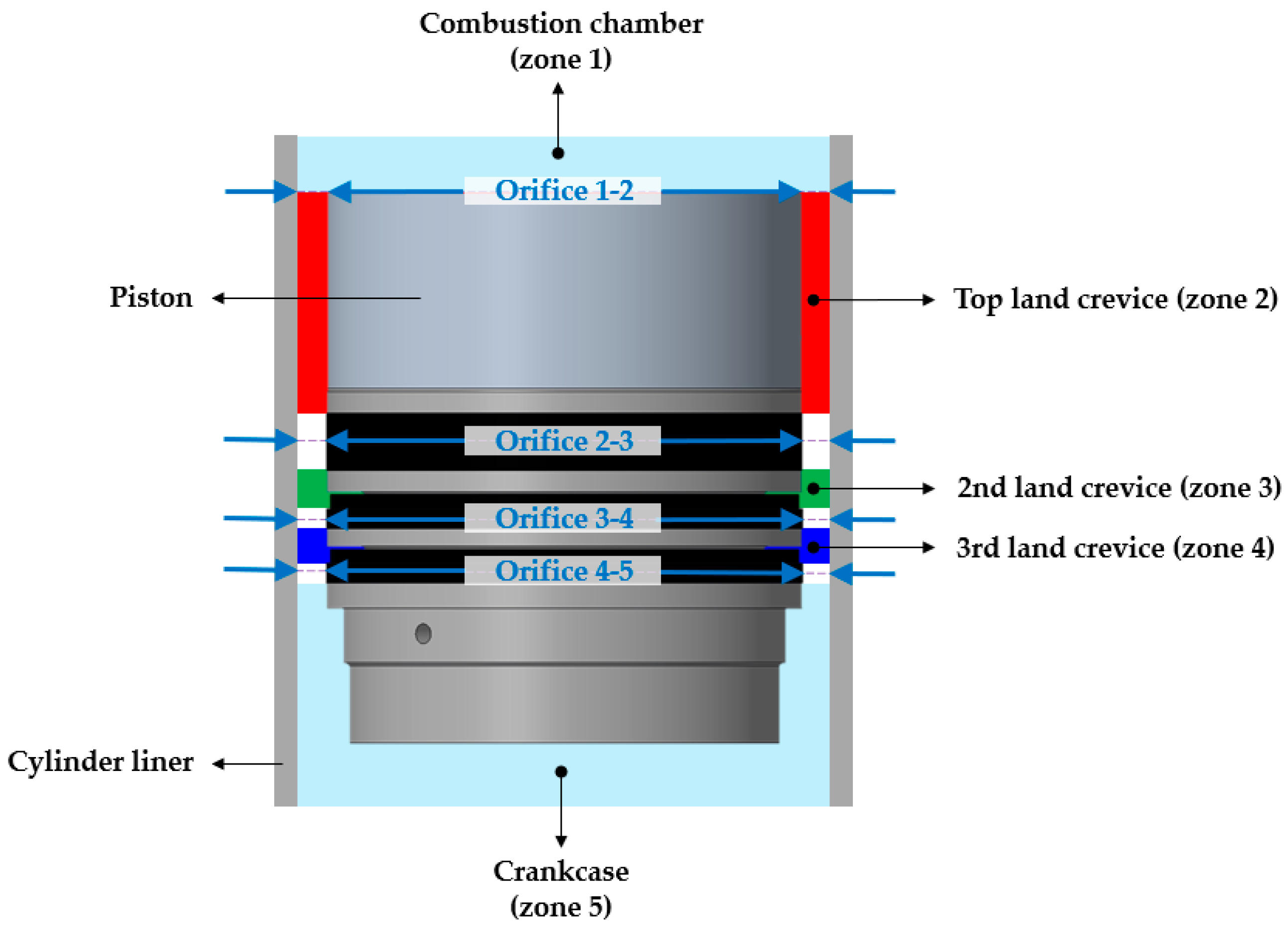
In order to simulate the blow-by mass transfer occurring between the combustion chamber, the piston rings, and the crankcase, 3 + 2 mass exchanging connected zones were considered in the implemented model (as shown in Figure 2):
  • three zones called ‘active domains’, which are: the piston top land crevice (zone 2), second land crevice (zone 3), and third land crevice (zone 4);
  • two additional zones called ‘ambient domains’, namely the combustion chamber (zone 1) and the crankcase (zone 5), which are used to provide the active zones with the boundary conditions.
The number of selected zones for the modelling (three) is the minimum needed to simulate the filling/emptying cycles of the piston ring belt with respect to the combustion chamber as far as the presence of three different piston rings is concerned. This solution leads to a more accurate simulation of the flow dynamics during the blow-by loss/recover phases against the choice to reduce all the crevices to an equivalent single pressure loss. In fact, as previously highlighted in [8,9,10], the use of a reduced subset of those zones leads to significant over-estimation of the mass flow rate and mass loss/recover from/towards the combustion chamber.

2.2.1. Calculation of the Blow-by-Induced Mass Flow

The pressure-driven blow-by mass flow through the clearance between the cylinder liner wall and the piston ring belt was calculated via the classical equation of the isentropic flux through an orifice (Equation (1), [22]) obtained by combining the mass flow expression (gas density × orifice cross section area × gas velocity), the isentropic gas transformation hypothesis, and the Bernoulli’s equation. Then, the real mass flow is given by the product between the theoretical isentropic flux formula and the discharge coefficient of the orifice, namely the clearance between the cylinder liner wall and the piston rings. In Equation (1), d m / d θ is the gas mass flow in kg/deg, i and i + 1 are the indexes associated to the zones connected by the orifice, ω is the engine speed in deg/s, C D , i , i + 1 is the discharge coefficient of the orifice, A i , i + 1 is the cross section area, p   is the absolute pressure of the zone, β i is the pressure ratio between the two zones ( β i = p i + 1 / p i ), R is the gas constant, γ is the gas heat capacity ratio and T   is the temperature of the zone. The heat capacity ratio was evaluated at each time step depending on the temperature of the zone according to the temperature-dependent correlations in [23].
d m i , i + 1 d θ = { 1 ω C D , i , i + 1   A i , i + 1   p i   2   γ R   T i ( γ 1 )   [ ( β i ) 2 γ ( β i ) γ + 1 γ ]   , β i 1 , β i > ( 2 γ + 1 ) γ γ + 1 1 ω C D , i , i + 1   A i , i + 1   p i     γ R   T i ( 2 γ + 1 ) γ + 1 γ 1   , β i 1 , β i ( 2 γ + 1 ) γ γ + 1 1 ω C D , i , i + 1   A i , i + 1   p i + 1   2   γ R   T i + 1 ( γ 1 )   [ ( 1 β i ) 2 γ ( 1 β i ) γ + 1 γ ]   , β i > 1 , β i > ( 2 γ + 1 ) γ γ + 1 1 ω C D , i , i + 1   A i , i + 1   p i + 1   2 γ R   T i + 1   ( 2 γ + 1 ) γ + 1 γ 1 , β i > 1 , β i ( 2 γ + 1 ) γ γ + 1
The expression of the real mass flow changes whether the flow direction (Equation (1), second column β i condition) is direct or inverse, and the flow condition is unchoked or choked (Equation (1), third column β i condition). According to the sign of the mass flow, the flux can be:
  • direct (if positive), describing the occurrence of blow-by-induced mass loss from the zone i towards the zone i + 1, e.g., gas flow from the combustion chamber towards the piston top land crevice;
  • inverse (if negative), describing the occurrence of blow-by-induced mass recover in the zone i from the zone i + 1, e.g., gas backflow from the piston top land crevice to the combustion chamber.
The discharge coefficient C D in Equation (1) was used as a tuning parameter, and it was calibrated as a single constant steady-state value that ensured the minimization of the error on the pressure trace between experiments [14,15] and simulations during the validation step (see Section 3.1). The tuned values of the discharge coefficients at both motored and firing conditions for each orifice are listed in Table 3. In Table 3, it is visible that the discharge coefficient of the orifices at firing conditions are larger with respect to those at motored conditions. This result is consistent with the discharge coefficient analysis presented in [24], in which the authors have shown that the discharge coefficient can be seen as the sum of a fixed contribution K , and a second contribution which is Reynolds-dependent as 1 / R e . Focusing on the orifice’s Reynolds variation between motored and firing conditions, as far as the combustion is concerned, the higher gas and piston temperature has the following effects which should be considered: (i) the reduction of the density and the increase of the viscosity of the gaseous phase; (ii) the reduction of the orifice flow area due to the thermal expansion of the solid material. Moreover, since the pressure in the rings increases according to that of the cylinder, the pressure difference-induced gas velocity through the rings does not change significantly with respect to the other three parameters. As a result, the Reynolds number at firing conditions will be lower, thus, the discharge coefficient will be higher. It is also underlined that the tuned values reported in Table 3 are consistent with respect to the typical range (0.6–0.85) reported in similar works [8,25]. As a further proof of the proposed discussion, one can observe that in the orifices from volumes 3 to 4, and from volumes 4 to 5, the discharge coefficients decrease towards lower values comparable with those of the motored case because of the lower temperatures in these volumes.
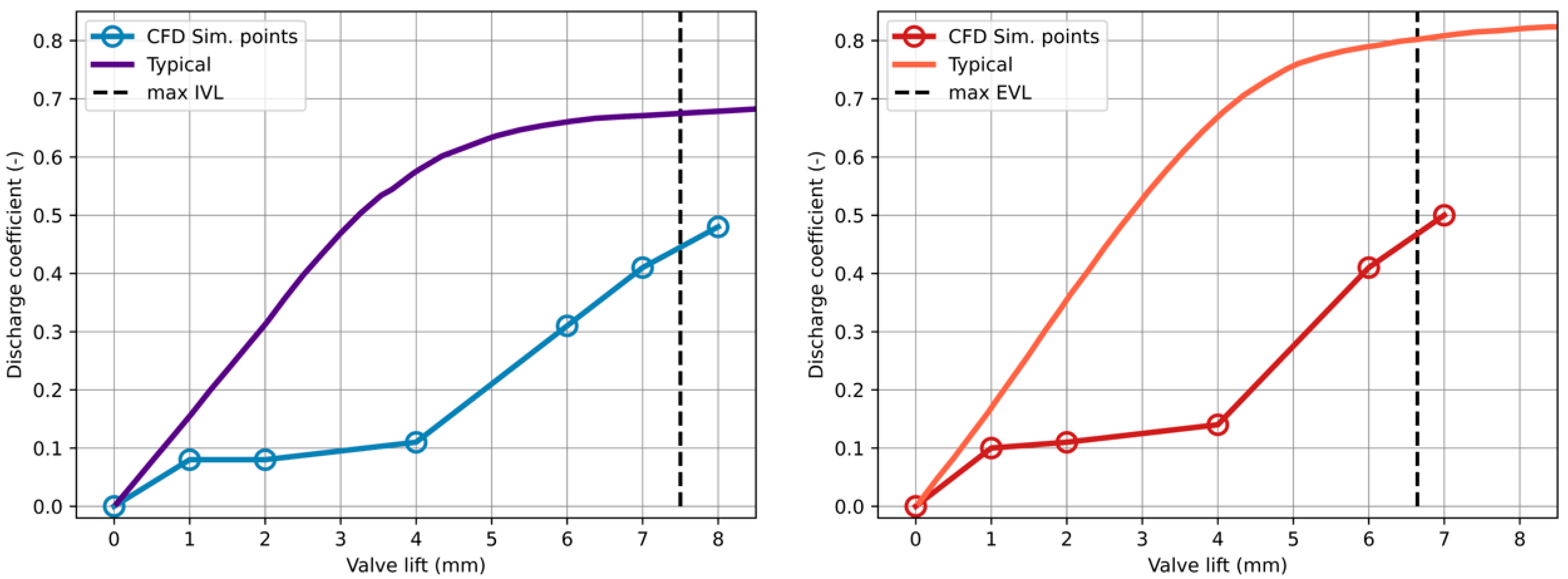
As mentioned, at each time-step the pressure and temperature values from the two zones of the ambient domain, i.e., the combustion chamber (zone 1) and the crankcase (zone 5), must be provided to determine the direction and the value of the mass flow at the two corresponding connected zones, the top land crevice (zone 2) and the third land crevice (zone 4), respectively. As the simulation case focused on an optical access engine mounted on a test rig, to calculate the contribution ± m 45 ˙ , the laboratory conditions (p = 1 bar, T = 298 K) were imposed as constant values. Concerning the combustion chamber (zone 1) for calculating the contribution ± m 12 ˙ , pressure and temperature are time-variable profiles which depend on the engine in-cylinder phenomena. It is underlined that the pressure profile of the zone 1, input of the quasi-dimensional blow-by model, must be that which describes the gross cycle, i.e., the in-cylinder pressure if the engine was not affected from blow-by. This is necessary in order to determine the effective pressure difference that drives the flow through the piston rings. The gross in-cylinder pressure profile was provided by the zero-dimensional engine open code OpenWAM [26], in which the layout of the experimental rig was reproduced (Figure 3). In order to provide robust gross pressure conditions to both the quasi-dimensional blow-by model and the CFD simulation in combined mode, it is necessary to ensure that the trapped air mass during the intake phase predicted by the engine zero-dimensional model is reliable. In this regard, both open and commercial engine zero-dimensional models require the so-called discharge coefficient profile of the valve curtain area during valves lift. Despite the fact that with the lack of tailored data, default or typical profile shapes can be put into the code for commercial-like engines, the same should not be applied to the reference optical engine due to the presence of specific geometric features, such as the flat piston crown and the ports’ masking. Therefore, the complete numerical CFD characterization of the ports was performed at reference conditions, i.e., system feeding with compressible dry air at 298 K, 1 bar under an inlet-outlet pressure difference of 115 mbar for the intake port, and 175 mbar for the exhaust port. Under these conditions, steady state simulations were run for different fixed valve lift positions.
For each simulated valve lift position, the discharge coefficient of the curtain area is calculated as the ratio between the mass flow rate recorded at the valve seat when the convergence is reached, and the theoretical mass flow calculated for the given pressure difference. For the sake of brevity, the results concerning the discharge coefficient profiles, which were provided as an input to OpenWAM, are collected in the Appendix A (Figure A1 and Figure A2).

2.2.2. Mass Flow-Induced Crevice Pressure Variation Calculation

Once the mass fluxes are known (Equation (1)), the pressure change into each of the simulation zones 2, 3 and 4 of constant volume V (which is the crevice volume), is computed by means of the differential form of the perfect gas law, as shown in Equation (2), in which V 2 , V 3 , V 4 are set to the values reported in Table 2, the value of the piston temperature ( T P ) depends on the case study (motored or firing, Table 1). As a result, the described problem is represented by a three-equation ordinary differential equation (ODE) implicit system (Equation (2)), which must be solved numerically for the pressure in each crevice. The solution of the latter was approached by using the Python built-in implementation of the second order Runge–Kutta method from the SciPy Integrator open library.
d d θ [ p 2 p 3 p 4 ] = 1 R   T P · [ 1 V 2 ( d m 1 , 2 d θ d m 2 , 3 d θ ) 1 V 3 ( d m 2 , 3 d θ d m 3 , 4 d θ ) 1 V 4 ( d m 3 , 4 d θ d m 4 , 5 d θ ) ]
Applying the Runge–Kutta method, the tool adopts the automatic refinement of the time step in order to accomplish given tolerance criteria between consecutive steps depending on the gradients. The solution was tuned by testing different values for the initial and the minimum allowed time step in order to achieve the best compromise between the non-oscillating behavior of the results, and fast computations. As a result, the initial computation step was set at 0.1 deg according to the sampling frequency of the gross pressure-temperature profiles from OpenWAM, whilst the minimum allowed step was set at 0.01 deg. The initial solution array for the crevices pressure was guessed as follow: the cylinder pressure is imposed into the top land crevice, whilst the crankcase pressure (ambient pressure) is imposed into the second and third top land crevices.

2.2.3. Post-Processing of the Numerical Solution

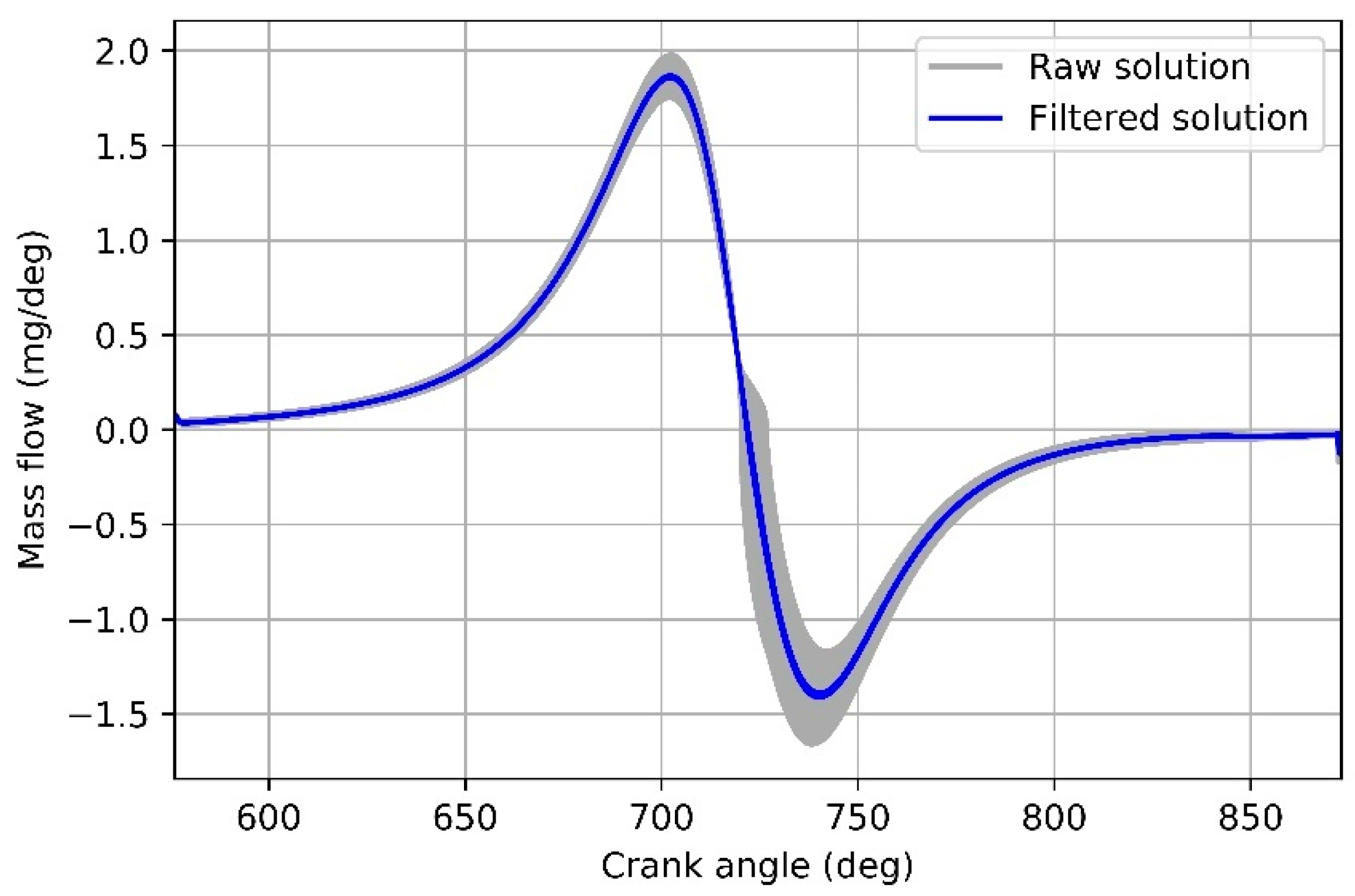
The raw profiles returned from the Runge–Kutta numerical solver were highly noisy. This behaviour is a significant concern, especially if one needs to use the code in combined mode, because providing the inlet/outlet boundary of a CFD domain with highly noisy conditions would promote convergence issues. It is highlighted that due to the automatic gradients-driven domain refinement applied by the adopted Runge–Kutta solver, the output pressure and mass flow profiles were characterized by non-uniformly distributed points. In light of the above, a custom implementation of a Savitzky–Golay filter was performed in order to smooth the model’s outputs while approaching the non-uniform distribution of the data. To this aim, the matrix form proposed by Sadeghi and Behnia [27] to determine the coefficients of the filter regardless of the input sampling was followed. In the final architecture, a second order filter (2nd degree polynomial) was chosen, having shown to be the best trade-off between accuracy (lower mean squared error in least square approximation) and computation cost, whilst the window length was set to 400 because of the large signal-to-noise ratio of the output returned by the model. Figure 4 displays the result of the applied filter to the noisiest output, i.e., the cylinder mass flow through the top ring. The grey area is drawn up by the large number of dense noisy points from the raw signal whilst the blue curve is the filtered signal.

2.2.4. Calculation of the Blow-by-Induced Cylinder Net Pressure

The estimation of the blow-by-induced pressure into the engine cylinder (Equation (3)), namely the effective pressure into the combustion chamber of the real engine ( p n e t ), is obtained by scaling the gross pressure ( p 0 ) at each time-step by the ratio between the gaseous mass that is still into the cylinder after the blow-by loss/recover, which was called net mass ( m n e t ), and the gaseous mass that would be trapped into the cylinder if no blow-by occurs ( m 0 , gross cycle).
p n e t = p 0 m n e t m 0
At each time step the present net mass ( m n e t ) is determined by adjusting the net mass calculated at the previous time step by considering the mass flow between the cylinder (zone 1) and the piston top land crevice (zone 2) due to the blow-by. As the initial condition, the mass trapped at the intake valve closing recorded for the gross cycle was considered ( m 0 ) since, at that engine phase, the blow-by losses are negligible, thus, gross and net conditions are almost the same.
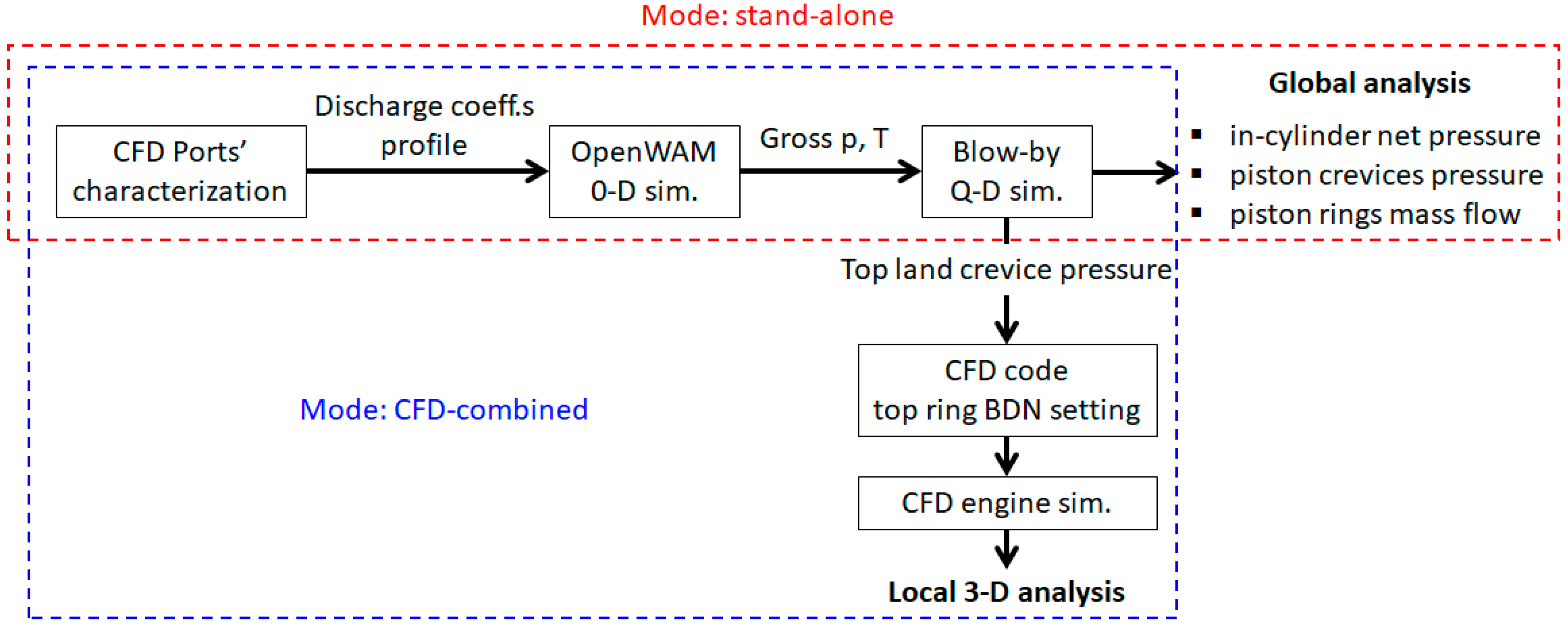
The described model is able to satisfy two different requests, working in two different modes: (i) stand-alone configuration, if the model is charged to directly simulate given engine operating conditions, and to return the afore-mentioned profiles; (ii) combined configuration, if the main task of the model is to provide the pressure profile into the top land crevice as a boundary condition on the blow-by bounding surface to the CFD simulation of the reference engine, integrating the mass/energy flux in a physical manner through the clearance of the combustion chamber. For the sake of clarity, the workflow of the method for the two modes is reported in the Appendix A in Figure A3.

2.3. CFD Simulation Methodology

Three-dimensional CFD simulations were performed with the commercial code AVL-FIRE v2014. In the computational mesh (Figure 5), the average cell size was set at 1 mm and it was fined up to 0.125 mm into the ring below the flat piston crown representing the fluid volume available in the top land crevice. It must be underlined that in order to run the present blow-by model in the CFD combined mode, the bottom surface of the simulated blow-by volume, i.e., the circular crown cross section of the top ring, was initialized as an inlet/outlet boundary on which the offline calculated pressure profile into the top land crevice was imposed. The main features of the mesh and of the simulation are summarized in Table 4. The fuel used in both experiments and simulations is commercial gasoline.
It is underlined that the model by Bianchi et al. [28], adopted via user file for the spray injection and breakup, was tuned and validated against in-vessel spray experimental data from [30,31]. For the sake of brevity, the spray validation is not reported since it is not the topic of the present work. However, it is reported that the CFD results with respect to the time-averaged droplets diameter and velocity from optical measures recorded at 15 and 20 mm downstream from the nozzle tip were characterized by relative errors around 3–5% and 1–6%, respectively.

3. Results

In this section the simulation results from both CFD and the quasi-dimensional model are reported. Firstly, the blow-by model in stand-alone mode is validated against experimental data at both motored and firing conditions. Once the reliability of the model in stand-alone mode was proven, the effect of different relevant engine conditions on the blow-by-induced collateral mass and heat transfer is discussed. In particular, the quasi-dimensional model in stand-alone mode was used to test different values of the engine speed (from 1100 r/min to 1500 r/min) and of the EGR amount (from 0%wt to 40%wt). Furthermore, a sensitivity analysis of the model to the temperature of the piston and the gas into the crevices is provided in order to discuss the confidence of the results depending on the choice of such value, which is usually not available, thus, it needs to be estimated. Indeed, the piston temperature in optical engines is usually lower than that of commercial-like engines due to the overall lower thermal regime imposed by limited firing time (around 1 min, after previous thermal conditioning). Finally, the combined mode is validated, and the results compared with the ones reached with the stand-alone mode.

3.1. Stand-Alone Configuration: Model Validation

In this section the validation of the quasi-dimensional blow-by model is focused on the stand-alone running mode. In this mode, the output of the model is mainly the behavior of the pressure into the combustion chamber (net pressure) and into the piston crevices, and that of the mass flow through the piston rings. With regards to the motored conditions, as visible in Figure 6a, a nice agreement between the predicted in-cylinder pressure and the experimental pressure trace was achieved.
As one can notice from Figure 6a, starting from 600 °CA (i.e., after the intake valve closing (Table 1)) the mass loss increases slowly, then, it becomes steep around 670 °CA, reaching the peak before the TDC (around 700 °CA). Despite the fact that one can expect the maximum blow-by mass flow at the TDC, the shift of the peak angle before the end of compression is mainly due to the mutual influence of the in-cylinder and the piston crevices pressures. In particular, the first crevice volume has a strong impact on the mass flow dynamics since it requires a significant time to be filled with new mixture. However, after 700 °CA, the volume is almost in a fluid-dynamics equilibrium with both the cylinder and the second land crevice, leading to the reduction of the pressure difference, which results in reduced flow rates. A further significant information from Figure 6a is that focusing on the top land crevice, the positive peak of the mass flow (mass loss) is greater than the negative one (mass recover). Moreover, the mass flow is still positive for a longer time than that during which it the recovery phase occurs (negative mass flow). As a consequence, the mass loss at the end of compression stroke, with respect to the trapped mass at IVC (intake valve closing), is approximately 20%, whilst an overall mass loss around 6% is predicted at EVO (exhaust valve opening) after the recovery phase during the expansion stroke.
It is worth mentioning that at the slope change of the mass flow during the recovery phase, in spite of the significant amount of backflow from the top land crevice to the cylinder, the mass flow through the second and the third piston rings is still positive (Figure 6b), hence the blow-by-induced flow through those rings is directed towards the crankcase and no mass recover occurs.
With regards to the firing simulation under the reference conditions presented in Table 1, the results are shown in Figure 7. Figure 7a displays that the model is able to predict the net pressure peak with sufficient accuracy, as reported for the motored conditions, whilst a slight over-estimation can be observed at the end of the compression stroke, likely due to the need to improve the capture of the effect of the wall heat transfer. Despite the fact that even in motored conditions (Figure 6a) the profile of the mass flow between the cylinder and the top land crevice was not symmetric with respect to the TDC, this effect is further enhanced in firing conditions (Figure 7a). The mass flow curve is characterized by two loss (positive) peaks: the first one, which is the lower, is consistent with that observed at the end of the compression stroke in motored conditions (around 2 mg/deg). Then, the slope increases significantly due to the initial large pressure difference between the cylinder and the top land crevice caused by the start of combustion and enhanced by the significant fluid-dynamics inertia of the latter because of its large volume (Table 2). The combustion-induced mass loss is more than doubled with respect to that of the motored conditions (almost 5 mg/deg). Figure 7a also displays that the combustion shifts the slope change of the mixture flow towards the expansion stroke. Under these conditions, the mass loss at the TDC is approximately 17%, which is 3% less with respect to motored operations because of the higher wall temperature (Equations (1) and (2)), whilst the maximum loss peak is around 30% of the trapped mass. The overall mass loss at EVO is around 14%, which is strongly higher than that of the motored case, resulting in a significant loss of ignitable mixture and heat generation, which one should accomplish by determining a new larger mass of injected fuel. The recovery phase is also highlighted for firing conditions, and mass flux behavior is comparable with that of the motored operative condition. Concerning the second and the third rings (Figure 7b), no significant differences of mass flow neither in the magnitude nor in the macroscopic behavior were detected.

3.2. Stand-Alone Mode: Simulation of New Points

The results of the proposed quasi-dimensional model run in stand-alone mode on new experimentally untested points are now discussed. The effect of the variation of some parameters was investigated.

3.2.1. Effect of the Piston Temperature

Before moving on to the discussion of the predicted effects of two key engine operating parameters (namely, engine speed and EGR charging), a sensitivity analysis by varying the chosen value of the piston temperature (which is also the temperature of the gases into the crevices according to the hypotheses listed in Section 2.1) is presented. Starting from the temperature with which the stand-alone mode was successfully validated in firing conditions (540 K), two additional values, one higher (570 K) and one lower (500 K) were considered in a reasonable range typical of engine firing full load operations. The importance of this sensitivity analysis lies in the fact that only the coolant temperature was recorded on the reference optical engine, whilst no direct measurements of the wall temperatures are available. It must be underlined that the lack of accurate information on the wall temperatures is quite common in the every-day practice of engine test bench research. Thus, proving the confidence of the predicted in-cylinder net pressure, even though the piston temperature input is a gross estimate, can be important to achieve a generally valid approach.
The result of the sensitivity analysis is shown in Figure 8, in which the blue curve refers to the benchmark simulation set (540 K) that was already validated in Section 3.1. From Figure 8, it is visible that there are slight differences between both the pressure and the mass flow curves for the three different temperatures that are mainly focused on the pressure peak, and on the mass loss peak, respectively. As a result, the small influence of the choice of the temperature value of the piston and of the gases flowing through the piston crevices on the predicted engine pressure was shown with respect to what was observed from the measurements. Thus, it can be emphasized that the sensitivity of the implemented model to the piston temperature chosen by the user, with the lack of measurements conducted on purpose (that can be quite expensive), is negligible as long as the assumed piston temperature value is in a reasonable range.

3.2.2. Effect of the Engine Speed

At first, the effect on the blow-by-induced mass flux and pressure loss is evaluated for different engine speeds: in particular, 1100 r/min and 1500 r/min engine speeds are investigated besides the 2000 r/min speed of the reference case. In this regard, Figure 9 shows the results of the engine speed analysis. The general behavior of the blow-by mass fluxes is in line with that presented in Figure 7. In Figure 9a, it is visible that the mass loss intensity decreases by increasing the engine speed because the higher the engine speed, the shorter the time available for the mixture to flow through the orifices.
Larger differences among the tested engine speeds can be seen at the two positive (loss) peaks, whilst the blow-by-induced mass recovery phase is weakly affected by this effect. As a result, reducing the engine speed leads to the increase of the overall mass losses (Figure 9b) since the imbalance between losses during compression stroke and recovery during expansion stroke is enhanced at a lower engine speed. As shown in Figure 9b, the mass loss among the tested speeds is almost the same until the combustion peak, though a difference of 5 percentage points in terms of additional mass loss, are found at EVO comparing the cases at 1100 and 2000 r/min.

3.2.3. Effect of the Charge Dilution

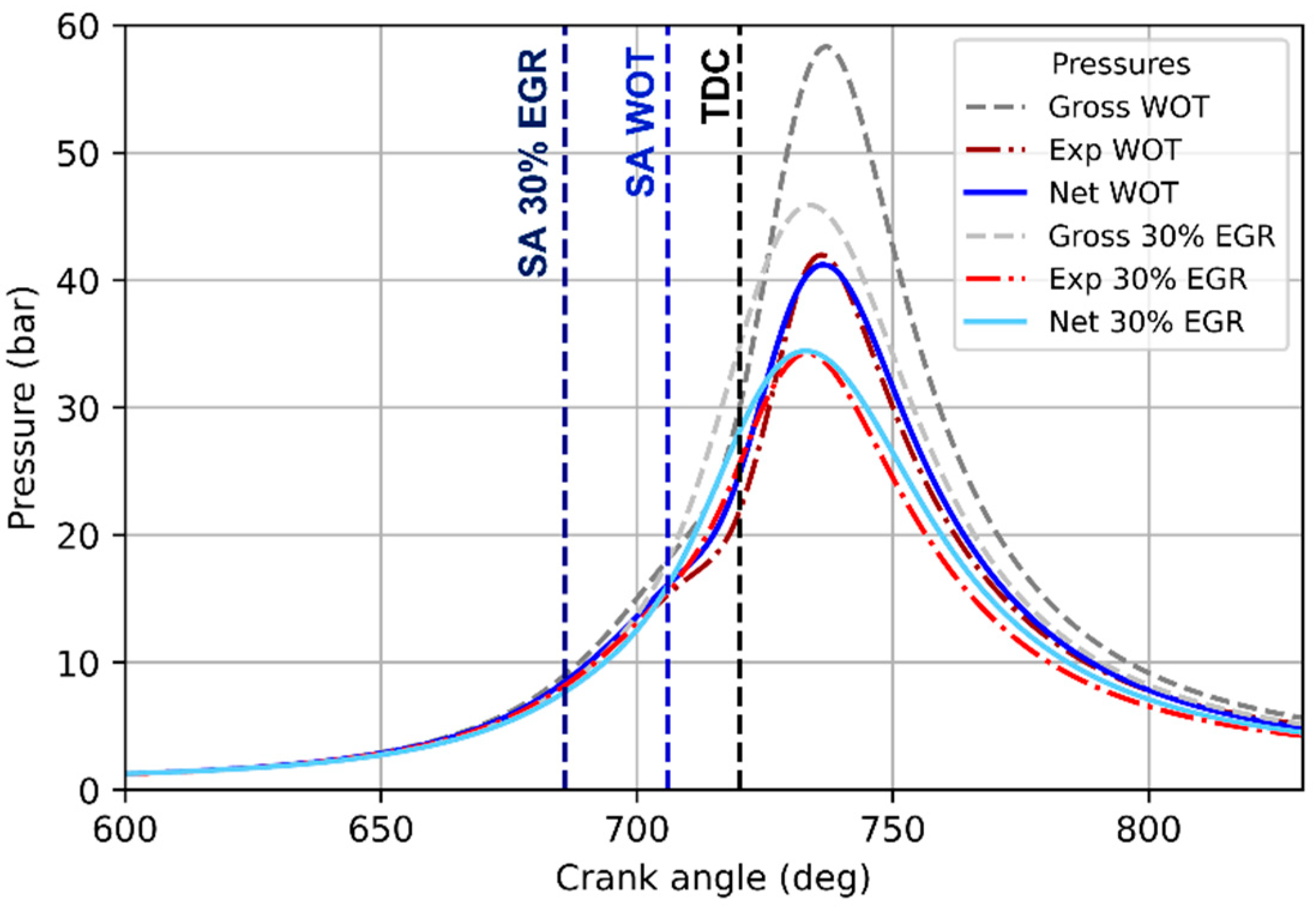
In this section, the results concerning the EGR-sweep ranging from 0%wt (engine operating at full load, only the internal EGR is present) to 40%wt (part load operations) are presented. Before moving on to the discussion of the results, it is important to clearly frame the aim of this analysis. As far as stabilizing the combustion process in highly diluted environment is mandatory in order to achieve both reduced heat losses and pressure losses in throttled operations, the reproduction of the EGR effect is important. Since the reference optical engine at the rig can actually be run with only two EGR configurations while maintaining confidence on the quantity of recirculated exhausts, namely 0% (WOT) and 30%wt (recirculation valve completely open), the ability of the model to capture the EGR effect would allow the mapping of the engine behavior in new points with different EGR values.
Firstly, Figure 10 shows the comparison between experimental and stand-alone numerical results for the two realizable EGR levels, i.e., 30%wt at part load and 0%wt at full load. It is visible that for the highly diluted environment, as well as shown at stoichiometric conditions, the use of the assumed gross in-cylinder pressure together with the implemented quasi-dimensional model allows for the capture of the engine’s overall indicating behavior. Then, the results of the EGR-sweep from 0%wt to 40%wt can be seen in Figure 11, in which the part load simulations (non-zero EGR points) were run considering a fixed spark timing set at that used for the validated experimental reference case EGR 30%, namely 34 deg before TDC. Figure 11a shows that at part load, operations richer in EGR are characterized by slightly higher pressure from the TDC to the peak due to the compression of the larger trapped mass at IVC. However, the blow-by mass flow profiles through the piston top ring (Figure 11a, dashed lines) are weakly affected by the EGR. As a result, as can be observed in Figure 11b, for similar behavior of the mass exchange with the top land crevice, the lower the operated EGR (thus the overall in-cylinder mass), the higher the mass loss.
Due to the weak effect of the EGR on the stand-alone blow-by model, one can expect that for robust input gross conditions, the global analysis in new EGR points performed with the implemented methodology is reliable.

3.3. Combined Configuration: Model Validation

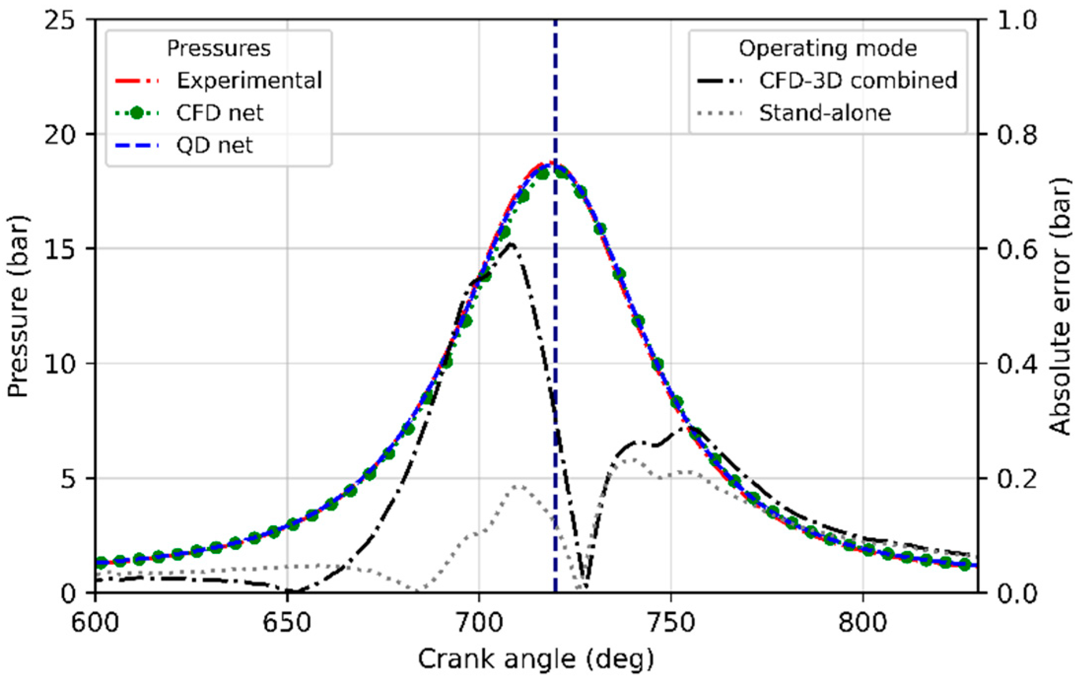
The validation of the offline integration of the proposed model with the commercial CFD code AVL-FIRE v2014 is presented in this section for both the motored and the firing reference conditions. It is remembered that the coupling between the quasi-dimensional model and the CFD code is applied by constraining the pressure on the top ring boundary surface of the computation mesh with the pressure profile of the top land crevice returned by the blow-by model. With regards to the motored conditions, Figure 12 shows the comparison between the net pressure from the code run in stand-alone mode, the simulated pressure by the CFD code in combined mode, and the experimental curve. It is visible that the CFD pressure trace of the engine blow-by simulation in motored conditions is in solid agreement with experiments as well as that predicted by the blow-by code run in stand-alone mode. The profile of the absolute pressure difference between simulations and experiments highlights that the combined mode suffers from a slight prediction performance derating in the last part of the compression stroke with respect to the stand-alone mode, likely due to the lack of a direct coupling between the top land pressure profile and the instantaneous in-cylinder pressure. The performance of the two modes in the recovery phase is almost the same. However, absolute difference below 1 bar are reached throughout the simulated high part of the engine cycle.
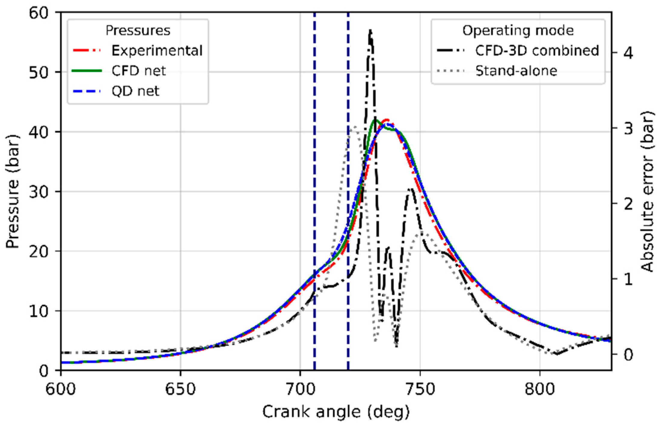
With regards to the firing conditions, the results returned by the combined mode are reported in Figure 13. The shape of the absolute pressure difference profiles associated to the combined and stand-alone modes are consistent with each other. The profile from the combined mode is in line with that from the stand-alone mode, in particular during expansion stroke, whilst significant differences can be observed at the end of the compression stroke and at the spark timing.
With regards to the former, the net pressure difference profile of the combined mode is greatly lower (<1 bar) than that of the stand-alone mode (1–3 bar) mainly due to the higher accuracy of the complex models implemented in the CFD code to simulate the heat transfer. With regards to the spark timing, the combined mode suffers from a greater net pressure difference peak (around 4 bar vs. 3 bar) due to the presence of the M-shape of the curve’s peak, which can, however, be corrected by putting more efforts in the CFD tuning step. The combined mode allows the effect of the blow-by-induced losses and recovery on the local mixture distribution.
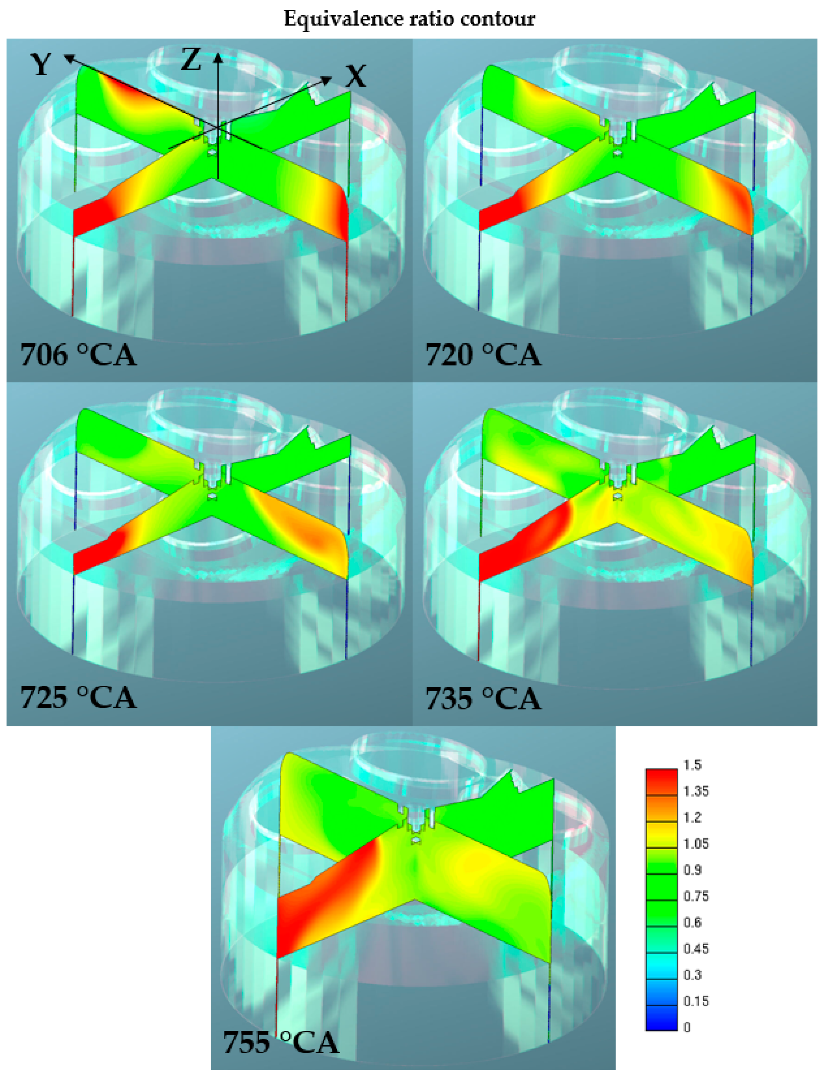
Figure 14 shows cross-planes sections of in-cylinder equivalence ratio (i.e., normalized fuel-air ratio) for different angles from the spark timing to the MFB90 (90% mass fuel burned).
It can be seen that at the spark timing the mixture quality into the top land crevice is non-symmetric along both the XZ and YZ cross-planes. Whilst the non-symmetric distribution could be expected along XZ due to the spray pattern which enhances the spray wall impingement against the liner at X-, the distribution along YZ is also non-symmetric (rich mixture 1.5 at Y−, lean mixture 0.8 at Y+), likely due to the transport of rich pockets by the swirl motion. From 720 to 725 °CA, almost pure air is recalled from the top ring boundary into the crevice (blue area). At 735 and 755 °CA, which are associated respectively to the MFB50 and MFB90, a local influence of the mass composition can be observed between the top land crevice and the cylinder. During recovery phase, the volume which was directly hit from the spray is still rich, leading to the consequence enrichment of the in-cylinder zone above it (735–755 °CA), allowing the match between the latter rich pocket of mixture and the flame, resulting in the M-shape pressure peak seen in Figure 14. Moreover, the non-symmetric YZ behavior is confirmed in the recovery phase, resulting in a slight leaning at the Y− and vice-versa at the Y+, giving proof of the importance of carrying out CFD simulations to account for these phenomena.

4. Discussion

This work proposes a fast and reliable methodology to evaluate blow-by mass and pressure losses by means of a quasi-dimensional model implemented in Python 3. The model returns the in-cylinder net pressure curve, and the blow-by-induced mass flux and pressure into the piston crevices. The development of such a model was aimed at providing a tool able to support both fast in-cylinder indicating analysis, and three-dimensional CFD simulations of optical engines typically affected by significant blow-by phenomena due to the installation of the optical equipment. After the use of the model under both motored and firing conditions to reproduce reference experimental data referred to a real optical engine, the methodology can be considered validated for both the two aims conceived, i.e., a stand-alone tool, and supporting device for CFD simulations comprising the piston crevices. With respect to the experimental data, absolute pressure differences below 1 bar were observed under motored conditions, in which the physics to simulate are quite simple, whilst maximum differences between 3–4 bar were detected under firing conditions around the combustion pressure peak. Focusing on the combined mode, it can be said that the offline integrated methodology was successfully implemented, allowing the computation time saving with respect to an online coupling between the user code and the CFD code at the cost of a slight accuracy derating around the early combustion development. The three-dimensional results from the analysis of the combined simulation highlighted that the axial extension of the blow-by segment added to the computational mesh is still an ongoing issue, strongly driven from the trade-off between computing cost and local predictivity of the mixture composition in the top land surrounding area. In future works, the extension and test of the blow-by volume to different lengths is planned in order to achieve a deeper knowledge of the effect of the blow-by on potential delayed combustion above the piston crown, and the corresponding effect on the combustion behavior and optical diagnostics. Moreover, the design of experiment tools will be applied for planning targeted operative conditions to ensure extensive validation of the model and provide a solid basis for choosing tailored solutions for fundamental optical investigations.

Author Contributions

Conceptualization, V.M. and A.I.; methodology, V.M., S.F., G.C. and C.A.; software, V.M. and C.A.; validation, E.D.R., V.M. and A.I.; writing—original draft preparation, E.D.R.; writing—review and editing, V.M., G.C. and A.I.; visualization, E.D.R. and G.C.; supervision, G.M.B. and S.F.; project administration, G.M.B. and S.F. All authors have read and agreed to the published version of the manuscript.

Funding

This research received no external funding.

Institutional Review Board Statement

Not applicable.

Informed Consent Statement

Not applicable.

Data Availability Statement

Data will be available upon reasonable requests.

Conflicts of Interest

The authors declare no conflict of interest.

Appendix A

In this appendix, the results regarding the discharge coefficient profiles obtained from the steady state CFD simulations at fixed valve lift positions are described. The simulations were performed with the same mesh shown in Figure 5, but without the clearance volume. The resulting discharge coefficients of the optical engine are shown in Figure A1 with dotted-solid lines. The initial flat behavior of the discharge coefficients from the very early lifts to half of the valve lift is due to the ports’ masking: the valves lie in the masked zone until they reach a lift of 4 mm. In the latter interval, the curtain area remains almost constant (Figure A2) since the reference optical engine is dramatically different from typical engines.
Figure A1. Simulated discharge coefficients (dotted-solid lines) for the intake port (left) and the exhaust port (right) of the optical engine. The maximum valve lift according to the engine valve law is reported in dashed black. The typical profiles of commercial engines are also reported for the sake of comparison (solid lines).
Energies 14 08566 g0a1
Figure A2. Schematic view of the variation of the valve curtain area for increasing valve lift and the effect of the port’s masking on it. Valve lifts from 1 mm to 6 mm are reported as examples.
Energies 14 08566 g0a2
After 4 mm, the discharge coefficient increases according to the increment associated to the cross-section flow area once the valve has exited the masking volume. For the sake of comparison, Figure A1 also displays, in solid lines, the typical discharge coefficient profile of commercial engines. Those curves were included in order to emphasize the need to perform this characterization step before generating the initial and boundary conditions.
Figure A3. Scheme of the blow-by methodology workflow. The steps of the stand-alone mode are included in the red square, those of the combined mode are in the blue square.
Energies 14 08566 g0a3

References

  1. Robertson, D.; Prucka, R. A Review of Spark-Assisted Compression Ignition (SACI) Research in the Context of Realizing Production Control Strategies. SAE Tech. Pap. 2019. [Google Scholar] [CrossRef]
  2. Polovina, D.; McKenna, D.; Wheeler, J.; Sterniak, J.; Miersch-Wiemers, O.; Mond, A.; Yilmaz, H. Steady-State Combustion Development of a Downsized Multi-Cylinder Engine with Range Extended HCCI/SACI Capability. SAE Int. J. Engines 2013, 6, 504–519. [Google Scholar] [CrossRef]
  3. Temel, V.K.; Sterniak, J. Characterization of SACI Combustion for Use in Model Based Controls. SAE Tech. Pap. 2014. [Google Scholar] [CrossRef]
  4. Aengeby, J. Closed Loop Control of the Combustion Phase in SI Engines Using Alternative Fuels. SAE Int. J. Adv. Curr. Pract. Mobil. 2020, 3, 312–319. [Google Scholar] [CrossRef]
  5. Overbrueggen, T.V.; Braun, M.; Klaas, M.; Schroder, W. Experimental Analysis of the Impact of Injected Biofuels on In-Cylinder Flow Structures. SAE Int J. Engines 2016, 9, 1320–1348. [Google Scholar] [CrossRef]
  6. Barroso, P.M.; Ribas, X.; Pita Sr, M.; Dominguez, J.; De Seia, E. HD Diesel Engines Development for Alternative Fuel Use. SAE Int J. Engines 2015, 8, 326–340. [Google Scholar] [CrossRef]
  7. Masuda, T. Experiment on the Rate of Blow-by in a Spark Ignition Engine. Bull. JSME 1960, 3, 104–111. [Google Scholar] [CrossRef] [Green Version]
  8. Aghdam, E.A.; Kabir, M.M. Validation of a blowby model using experimental results in motoring condition with the change of compression ratio and engine speed. Exp. Therm. Fluid Sci. 2010, 34, 197–209. [Google Scholar] [CrossRef]
  9. Mahmud, Z.A. End Gas Autoignition and Knock in Spark Ignition Engines. Ph.D. Thesis, University of Leeds, Leeds, UK, 1999. [Google Scholar]
  10. Cairn, A. Turbulent Flame Development in a Spark Ignition Engine. Ph.D. Thesis, University of Leeds, Leeds, UK, 2001. [Google Scholar]
  11. Namazian, M.; Heywood, J. Flow in the Piston-Cylinder-Ring Crevices of a Spark-Ignition Engine: Effect on Hydrocarbon Emissions, Efficiency and Power; SAE Technical Paper 820088; SAE International: Warrendale, PA, USA, 1982. [Google Scholar]
  12. Kuo, T.; Sellnau, M.; Theobald, M.; Jones, J. Calculation of Flow in the Piston-Cylinder-Ring Crevices of a Homogeneous-Charge Engine and Comparison with Experiment. SAE Trans. 1989, 98, 1469–1482. [Google Scholar]
  13. Malagi, R.R. Estimation of Blowby in Multi-cylinder Diesel Engine Using Finite Element Approach. SAE Tech. Pap. 2012. [Google Scholar] [CrossRef]
  14. Irimescu, A.; Di Iorio, S.; Merola, S.S.; Sementa, P.; Vaglieco, B.M. Evaluation of compression ratio and blow-by rated for spark ignition engines based on in-cylinder pressure trace analysis. Energy Convers. Manag. 2018, 162, 98–108. [Google Scholar] [CrossRef]
  15. Irimescu, A.; Tornatore, C.; Marchitto, L.; Merola, S.S. Compression ratio and blow-by rates estimation based on motored pressure trace analysis for an optical spark ignition engine. Appl. Therm. Eng. 2013, 61, 101–109. [Google Scholar] [CrossRef]
  16. Breda, S.; D’Orrico, F.; Berni, F.; d’Adamo, A.; Fontanesi, S.; Irimescu, A.; Merola, S.S. Experimental and numerical study on the adoption of split injection strategies to improve air-butanol mixture formation in a DISI optical engine. Fuel 2019, 243, 104–124. [Google Scholar] [CrossRef]
  17. Merola, S.S.; Irimescu, A.; Vaglieco, B.M. Influence of water injection on combustion identified through spectroscopy in an optical direct injection spark ignition engine. Fuel 2020, 273, 117729. [Google Scholar] [CrossRef]
  18. Irimescu, A.; Marchitto, L.; Merola, S.S.; Tornatore, C.; Valentino, G. Evaluation of different methods for combined thermodynamic and optical analysis of combustion in spark ignition engines. Energy Convers. Manag. 2014, 87, 914–927. [Google Scholar] [CrossRef]
  19. Merola, S.S.; Irimescu, A.; Marchitto, L.; Tornatore, C.; Valentino, G. Effect of injection timing on combustion and soot formation in a direct injection spark ignition engine fueled with butanol. Int. J. Engine Res. 2017, 18, 490–504. [Google Scholar] [CrossRef]
  20. Irimescu, A.; Merola, S.S.; Tornatore, C.; Valentino, G. Development of a semi-empirical convective heat transfer correlation based on thermodynamic and optical measurements in a spark ignition engine. Appl. Energy 2015, 157, 777–788. [Google Scholar] [CrossRef]
  21. Bowditch, F. A New Tool for Combustion Research A Quartz Piston Engine. SAE Tech. Pap. 1961. [Google Scholar] [CrossRef]
  22. Heywood, J.B. Internal Combustion Engine Fundamentals; McGraw-Hill Education: New York, NY, USA, 1988; p. 226. [Google Scholar]
  23. Green, D.W.; Southard, M.Z. Perry’s Chemical Engineers’ Handbook, 9th ed.; McGraw-Hill Education: New York, NY, USA, 2018. [Google Scholar]
  24. Baker, R.G. Flow Measurement Handbook: Industrial Designs, Operating Principles, Performance, and Applications; Cambridge University Press: Cambridge, UK, 2000. [Google Scholar]
  25. Brahma, I. Measurement and Prediction of Discharge Coefficients in Highly Compressible Pulsating Flows to Improve EGR Flow Estimation and Modeling of Engine Flows. Front. Mech. Eng. 2019, 5, 25. [Google Scholar] [CrossRef]
  26. OpenWAM. Available online: http://openwam.webs.upv.es/docs/ (accessed on 3 December 2021).
  27. Sadeghi, M.; Behnia, F. Otpimum window length of Savitzky-Golay filters with arbitrary order. arXiv 2018, arXiv:1808.10489. [Google Scholar]
  28. Brusiani, F.; Bianchi, G.M.; Tiberi, A. Primary Breakup Model for Turbulent Liquid Jet Based on Ligament Evolution. SAE Tech. Pap. 2012. [Google Scholar] [CrossRef]
  29. Pulga, L.; Bianchi, G.M.; Ricci, M.; Cazzoli, G. Development of a Novel Machine Learning Methodology for the Generation of a Gasoline Surrogate Laminar Flame Speed Database under Water Injection Engine Conditions. SAE Int. J. Fuels Lubr. 2019, 13, 5–17. [Google Scholar] [CrossRef]
  30. Marchitto, L.; Merola, S.; Tornatore, C.; Valentino, G. Experimental Study on the Spray Atomization of a Multi-hole Injector for Spark Ignition Engines Fuelled by Gasoline and n-Butanol. SAE Tech. Pap. 2014. [Google Scholar] [CrossRef]
  31. Marchitto, L.; Valentino, G.; Merola, S.; Tornatore, C. Characterization of Alcohol Sprays from Multi-hole Injector for DISI Engines through PIV Technique. SAE Tech. Pap. 2015. [Google Scholar] [CrossRef]
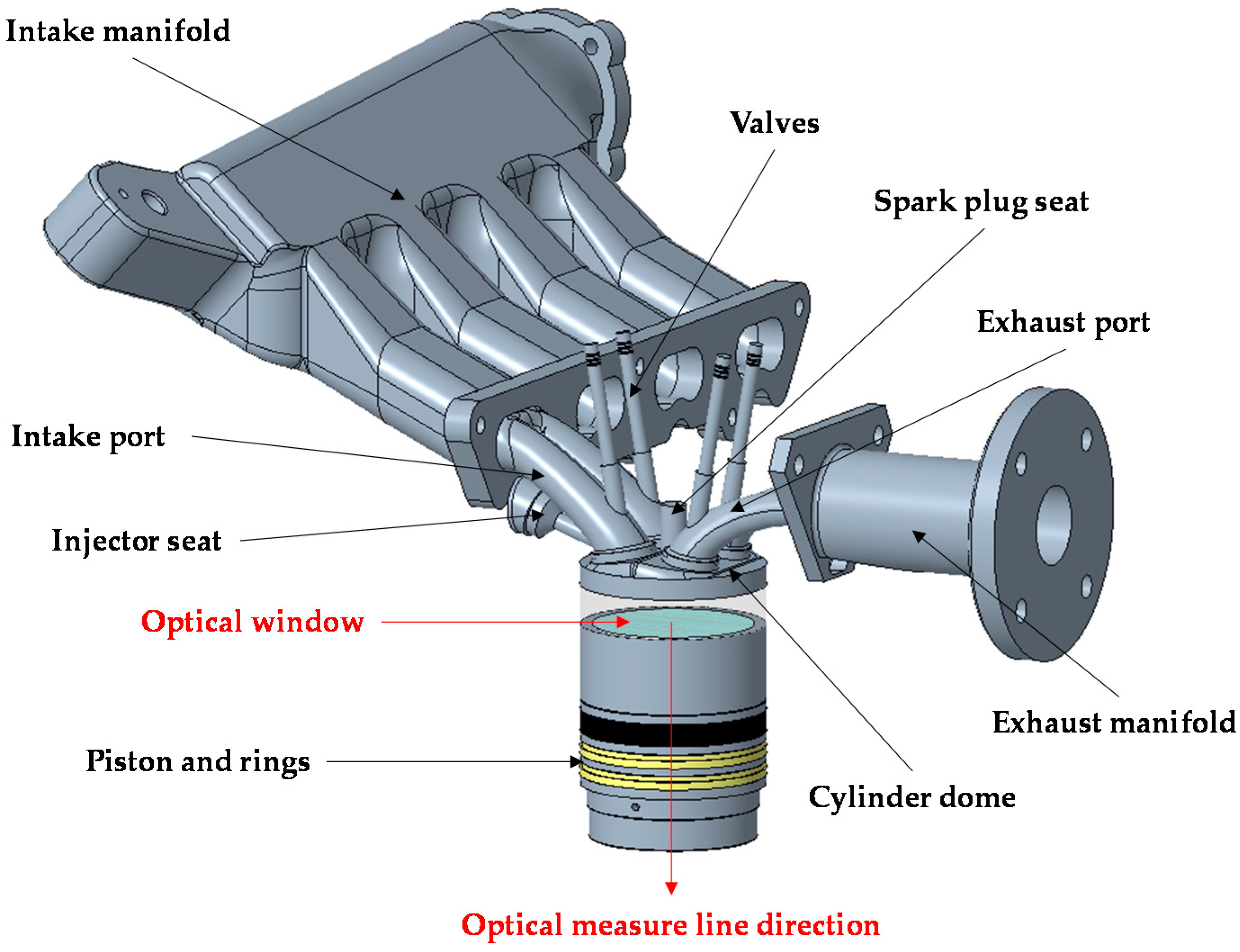
Figure 1. Overview of the CAD model of the experimental optical engine comprising the different components used for the numerical simulation. In particular, the quartz window installed on the piston is shown in light blue.
Energies 14 08566 g001
Figure 2. Schematic representation of the three active zones (red, green, blue) and the two ambient zones (light blue) of the computation domain. The CAD model of the piston and a schematic view of the cylinder liner are also shown.
Energies 14 08566 g002
Figure 3. Layout of the optical engine set in the OpenWAM environment.
Energies 14 08566 g003
Figure 4. Comparison between the raw (grey) and the filtered (blue) mass flow rates between the engine cylinder and the top land crevice in motored conditions.
Energies 14 08566 g004
Figure 5. Computational mesh of the experimental optical engine, details of the refined zones in the yellow outlines.
Energies 14 08566 g005
Figure 6. Comparison between simulated (solid lines) gross, simulated net, and experimental (dashed red line) pressure curves in stand-alone mode in motored conditions. The blow-by flow rate between the cylinder and the top land crevice is also reported (blue dashed line) (a). Pressure (solid lines) and blow-by flow rate (dashed lines) through the second and third land crevices (b).
Energies 14 08566 g006
Figure 7. Comparison between simulated (solid lines) gross, simulated net, and experimental (dotted red line) pressure curves in stand-alone mode in firing conditions. The blow-by flow rate between the cylinder and the top land crevice is also reported (blue dashed line) (a). Pressure (solid lines) and blow-by flow rate (dashed lines) through the second and third land crevices (b).
Energies 14 08566 g007
Figure 8. Simulated effect of different piston temperature values on the in-cylinder pressure (solid lines) and on the mass flow through the piston top ring (dashed lines).
Energies 14 08566 g008
Figure 9. Simulated effect of the engine speed on the in-cylinder pressure (solid lines) and on the mass flow (dashed lines) through the piston top ring (a) and the associated mass loss profiles (b).
Energies 14 08566 g009
Figure 10. In-cylinder pressure comparison between experimental (dotted lines) and numerical (solid lines) at full load (WOT) and part load with 30% of EGR. The respective gross pressure curves (dashed lines) are also reported. Vertical dashed lines indicating the spark timing of both the validation cases, and the top dead center are also shown.
Energies 14 08566 g010
Figure 11. Simulated effect of the EGR on the in-cylinder pressure (solid lines) and the mass flow through the piston top ring affected by blow-by (a) and the associated mass losses profile (b).
Energies 14 08566 g011
Figure 12. Comparison between the pressure curve predicted by the model applied in stand-alone (dotted blue line) and combined (dotted green line) modes with respect to experimental data (dotted red line) in motored conditions. The profile of the absolute error of the two modes (dotted gray for stand-alone, dotted black for combined) is also reported in the second y-scale. The TDC angle is indicated by the dashed blue vertical line.
Energies 14 08566 g012
Figure 13. Comparison between the pressure curve predicted by the model applied in stand-alone (dotted blue line) and combined (dotted green line) modes with respect to experimental data (dotted red line) in firing conditions. The profile of the absolute error of the two modes (dotted gray for stand-alone, dotted black for combined) is also reported in the second y-scale. The SA angle and the TDC are indicated by the two dashed blue vertical lines.
Energies 14 08566 g013
Figure 14. Equivalence ratio (fuel-air ratio divided by the stoichiometric fuel-air ratio) evolution and effect of the blow-by for different angles on two different cross-planes (XZ, YZ).
Energies 14 08566 g014
Table 1. Geometrical and operating data of the reference experimental test bench engine. Timings given in crank angle degrees (°CA).
Experimental Test Bench Engine Data
Bore (mm)79.0
Stroke (mm)81.3
Conrod length (mm)143
Geometric compression ratio10.0
Number of valves4
Intake valves opening/closure (°CA)363/576
Exhaust valves opening/closure (°CA)207/360
Engine speed (r/min)2000
Fuel system100 bar DI wide spacing
FuelCommercial gasoline
SOI/EOI (°CA) 430/469
Engine loadMotored/Full load
Motored/Firing piston temperature (K)380/540
Spark timing (°CA)706
Table 2. Blow-by geometric parameters from the engine CAD model.
Crevice Volume Data (mm3)
GeometryReference Optical EngineCommercial Typical [8]
Top land 3468.4≈970
Second land 654.7≈353
Third land 654.7≈353
Ring Cross Section Area Data (mm2)
Cylinder-piston crown clearance74.2≈62.60
First ring12.4-
Second ring2.5≈0.95
Third ring2.5≈0.95
Table 3. Tuned values of the blow-by orifice discharge coefficients in motored and firing operations.
Orifice ID C D   M o t o r e d C D   F i r i n g
1 -> 20.60.85
2 -> 30.60.85
3 -> 40.60.7
4 -> 50.60.7
Table 4. List of the main CFD settings for the engine simulation. BDC is bottom dead center, TDC is top dead center.
Simulation ParametersSetup
CodeAVL-FIRE commercial
N. of cells 1.5M (BDC), 1M (TDC)
Base cell size 1.0 mm
Spark plug cell size0.25 mm
Injector zone cell size0.5 mm
Blow-by cell size0.125 mm
Turbulence modelRANS k-z-f
Spray break-up modelBianchi [28] tuned
Wall impingement modelKuhnke
Combustion modelECFM-3Z tuned
Ignition + laminar flame speedCustom [29]
Blow-by boundary temperaturePiston temperature
Publisher’s Note: MDPI stays neutral with regard to jurisdictional claims in published maps and institutional affiliations.