1. Introduction
To meet the challenging climate targets of the Paris agreement [
1] and the European Union framework [
2,
3] will most likely require large-scale employment of electric vehicles (EVs) over the coming decades. New EVs will entail a new electricity demand and charging infrastructure that must be integrated into the electricity supply system. The electricity supply system will, at the same time, be increasingly dependent on solar and wind power that will vary in production. Thus, if the integration of EVs comes with an appropriate strategy, the new EV demand could offer benefits in terms of flexibility of the load, e.g., demand response services and, possibly, also discharge back to the grid (i.e., vehicle-to-grid; V2G). It is therefore essential to investigate EV’s impact on the current and future electricity system. This can be accomplished by, for example, using electricity system optimisation models [
4,
5,
6].
Previous studies on modelling of the electricity system with the inclusion of charging of EVs in the models have based their EV driving demand mainly on data from travelling surveys, standardised driving cycles and one day measured driving distances [
7,
8,
9,
10,
11,
12,
13,
14,
15,
16,
17]. Thus in previous studies, due to the lack of detailed data on individual driving patterns, the heterogeneity of the EV fleet is aggregated to one entire EV fleet represented as “one huge battery” in these models. For example, Šare et al. [
10] are using traffic load measured for the Dubrovnik region for one specific day when modelling the electricity system in Ukraine. In Juul [
8] transport pattern is treated with average values based on statistical data from a Danish travel study. In Hadley et al. [
13] it was assumed that all vehicles plugged in at two different times of the day and remained plugged in until fully re-charged. Cai and Xu [
9] used large-scale individual-based trajectory driving data, in a case study of Beijing, to better understand the electrification of the taxi fleet. However, driving data to be used for electricity system optimisation models, including the whole passenger car fleet, needs to be randomly selected among all registered passenger car owners in order to capture the driving pattern.
Data from self-reported travelling surveys, the main methodology used in previous studies, often under-estimate the frequency of trips, focusing on the travel behaviors of persons during one day rather than on the movement patterns of cars over a longer time period [
18]. Elango et al. [
19] and Björnsson [
20] have shown that individual passenger car driving patterns vary considerably from day to day, which might be an important factor to include in the electricity system models, so as to estimate the flexibility in load that could be offered by the EV batteries over a time-frame of more than one day.
Schuller et al. [
11] and Taljegard et al. [
21] used to some extent detailed individual driving data in their modelling. Schuller et al. [
11] used one week of driving patterns with total 1000 different driving profiles from the German National Travel Survey to study the integration of wind and solar power with flexible EV charging. Taljegard et al. [
21] studied the North European electricity system using an optimisation model and a dataset of 426 representative passenger cars measured for 30–70 days per car in western Sweden. One drawback with the clustering method of representative vehicles used by Taljegard et al. [
21] is that it does not allow electricity storage in the vehicle batteries from one day to another.
A more detailed definition of individual car movement patterns than presented in previous mentioned studies can be achieved when using measurements of time and position using Global Positioning System (GPS) equipment over a sufficiently long time period (most likely several weeks). Two main reasons why electricity system models aggregate the individual EV driving demands and profiles to a single driving profile for the entire EV fleet represented as “one huge battery” without evaluating the consequences of this simplification are that:
Since previous studies in the literature does not including individual driving patterns, there might be a risk that they over-estimate the potential of using the EV batteries for optimised charging and V2G. This could be the case since a vehicle that is parked might be charging so as to supply an EV that is out driving. Therefore, it is important to investigate when an aggregated vehicle representation is a good proxy and when representation of individual driving patterns is needed in electricity system models to estimate the V2G potential of passenger EVs. More comprehensive energy system models than the one used in this study, that also include, for example, trade between regions or several sectors, might not be suitable for something other than an aggregated vehicle representation. However, it is still important to understand the impact of the simplification with an aggregated vehicle representation on the model results.
This study are aiming at filling this research gap by developing and comparing both an aggregated vehicle representation with individual driving profiles, as well as, comparing two different ways of including individual driving profiles in an optimisation electricity system model. This study investigates when the different approaches (i.e., an aggregated EV representation and individual driving profiles) can be a good enough proxy to represent EVs in electricity system models by comparing modeling results from model runs that includes the different approaches.
The electricity system model used in this study was designed so that all approaches could be run within a reasonable time-frame. In this study, the differences of including individual EV driving profiles compared to an aggregated vehicle representation in electricity systems models are analysed while varying a number of parameters that might affect the results. These parameters are, for example, the geographical scope, EV battery capacities, V2G implementation schemes, and charging infrastructure connection points.
2. Data and Model Description
Three different approaches to integrate EV in electricity system models are described in
Section 2.2. The approaches are (i) aggregated vehicle profile (AGG); (ii) representative daily driving profiles (DDP); and (iii) yearly driving profiles (YDP). DDP and YDP include individual driving patterns, while AGG uses only the values averaged from the measured individual driving patterns. The individual driving patterns is in this study taken from a dataset of 426 representative passenger cars measured with GPS for 30–70 days per car in western Sweden. More details of the dataset can be found in
Section 2.1.
To evaluate and compare these approaches, a cost-minimisation model of the electricity system (called ENODE) has been used in this study. ENODE is designed to analyse the electricity system in regions in Europe when meeting a strict CO
2 emission target. A general description of the model can be found in
Section 2.3. The way EVs (i.e., AGG, DDP, and YDP) are implemented in ENODE is described in
Section 2.4. The different approaches have methodological implications, such as differences in data and equations structure, as described in
Section 2.4.
2.1. The GPS Vehicle Data-set
Measured travelling patterns from a campaign conducted in the region of Västra Götaland (western part of Sweden) are used for the individual driving pattern in the modelling. These are GPS measurements of about 770 randomly chosen gasoline- and diesel-powered vehicles that completed 107,910 trips between years 2010 and 2012 [
20,
26]. The vehicles were randomly selected from the Swedish vehicle database.
Of the around 770 households that had GPS equipment sent to them, about 529 were logged for more than 30 days, and 426 of those 529 provided high-quality data (i.e., excluding some of the vehicles where too much data were missing due to problems with the GPS equipment such as lost contact in power supply or satellite connection). Extensive data cleaning, validation, and a deeper analysis of the representation of the GPS vehicle data-set were carried out by Björnsson [
20]. The regions are found to be reasonably representative for Sweden in terms of fleet composition, car ownership, household size, income, and distribution of cars in larger and smaller towns and rural areas [
20]. Each vehicle was measured for a period of about 2 months, although the 2-month periods occurred during different times of the year for the vehicles involved. In total, 27,879 logged days were included.
The GPS-data applied in this work to determine individual driving patterns includes data that are measured for several days in a row and that are representative for the population in a larger geographical region. Thereby this GPS-data set is so far unique and only available for one region in Sweden. Since no such data was available for the other regions investigated, we have assumed the same driving profiles for all regions investigated in Europe. Since data on individual driving patterns were only available for one region in Sweden and therefore applied also to the other regions investigated, this will obviously not consider national differences in the driving profiles. Thus, there may be regional differences affecting the driving patterns such as working hours, leisure time activities, as well as geographical factors like Sweden being a low population density country.
2.2. Description of EV Integration Approaches
Table 1 gives a summary of the three approaches to integrate EVs into electricity system models. Out of the three approaches to integrate EVs, DDP, and YDP include individual driving patterns, while AGG uses only the values averaged from the measured individual vehicles.
2.2.1. Aggregated Vehicle Profile (AGG)
AGG uses the values averaged from the measured individual vehicles. An extrapolation of the measured driving distance of about 2 months per vehicle in the GPS vehicle data-set to a full year of driving by using the measured period repeatedly, yields an average yearly driving distance of about 15,000 km per vehicle. With AGG, it is thereby assumed that all vehicles are driving 15,000 km per year. Furthermore, we used the 426 extrapolated vehicles to get the share of the vehicle fleet that are being parked each hour and being out driving each hour, respectively.
The GPS vehicle data-set comes from driving patterns of fossil fuel cars. Some of the driving distances are not possible for EVs, due to the limited range of EVs. From the GPS vehicle data-set, we have estimated how large share of the kilometers driven by the measured fossil fueled vehicles that could be covered with EVs. The share of the yearly kilometres that can be run on electricity per vehicle depends on the EV battery capacity, the assumed deployment of charging infrastructure and charging power. For example, the shares of the distances driven on electricity, when assuming a charging power of 7 kW, charging connection exclusively at the home location and applying 15, 30, and 85 kWh EV battery capacities, are 71%, 83%, and 94%, respectively (see
Figure A2 in
Appendix C).
The model optimises the charging and discharging to the grid of the aggregated EV battery with an hourly time resolution, and since this approach entails only an aggregated vehicle profile, it is assumed that a share of the fleet is parked and a share is out being driven. Therefore, with the AGG approach, there is the risk that a vehicle that is standing still can be charging for a vehicle that is out driving. Thereby over-estimating the potential to use the EV batteries for optimising the charging and for V2G. Data for how large share of the fleet that is parked, respectively out driving, each time-step in the model is based on data from the GPS vehicle data-set. The main benefits with AGG is that the approach can be used in most optimisation models, regardless of the size of the model.
2.2.2. Representative Daily Driving Profiles (DDP)
The aim of using DDP in the model is to account for individual driving profiles while still keeping the number of variables in the model relatively low. The DDP divides the measured vehicles into several daily driving profiles. For each representative driving profile and time-step, all the vehicles in that category are either being parked or out driving. This strategy thereby solves the problem associated with the AGG approach where the collective idle vehicle battery capacity can be charged even though the electricity is needed by vehicles that are on the road.
The GPS vehicle data-set consist of 27,879 measured days, including days during which the measured vehicles are driving, as well as, not driving. We call these 27,879 measured days for daily driving profiles. In the present work, a K-means clustering method [
27] is applied to determine (i) which of the daily driving profiles; (ii) how many of the daily driving profiles that is needed; and (iii) how these daily driving profiles should be weighted in relation to each other, to represent the curve of total number of daily driving profiles.
Figure 1 shows the total average daily driving distance over the day for sample sizes of 10, 50, 100, 200, and 500 representative days, as well as for the entire 27,879 measured days. Thus, approximately 200 representative days out of the total of 27,879 measured 1-day profiles are required for a reasonable representation in terms of both the driving distance and the shape of the average driving profile. Thus, in this study, the driving demand for EVs is approximated by 200 representative daily driving profiles.
The main drawback of the applied modelling approach (i.e., DDP) using representative daily driving profiles is that it does not allow for electricity storage in the vehicle batteries from one day to another. Thus, even though there is a good overall representation of the demand profiles from the representative days there is no information on the linkages between such representative days. The model also becomes more computationally demanding, as compared to AGG, due to the increased number of variables with DDP.
2.2.3. Yearly Driving Profiles (YDP)
The GPS vehicle data-set includes high-quality data for 426 gasoline- and diesel-driven vehicles measured for 30–73 days per vehicle, i.e., no vehicle has a full year of logging. An alternative approach to using representative daily driving profiles is to use the measured driving period per vehicle and extrapolate the data from the original period to 12 months. This means that the driving data for each vehicle are used repeatedly with respect to days of the week, such that the driving data have always the same weekday as the other load data. In this way, we get 426 yearly driving profiles.
Figure 2 shows, for the 426 yearly driving profiles, the share of the year being parked at the home location, all parking at stops longer than 6 h, and all parking at stops longer than 1 h. Large variability is seen between the 426 yearly driving profiles in terms of the numbers of kilometres driven per year (see
Figure A1 in
Appendix C) and the driving profiles and hours being parked per year (
Figure 2). This shows that the different driving profiles most likely need to be charged differently and have different conditions for participating in V2G.
The main advantage with this method is that the storing of electricity between days can be captured, reducing the risk of under-estimating the potential of optimised charging and V2G, compared to DDP. The main disadvantage with this approach is that more variables are needed in the model, which means that either the model takes longer time to run compared to AGG and DDP, or that less details are required in some other parts of the model.
2.3. General Model Description
The cost-minimisation model of the electricity system, ENODE, is both an investment and dispatch model designed to analyse investments in electricity generation capacities and storage technologies, and the hourly dispatches of different technologies. It is also a Greenfield model (i.e., assumes an empty system as the starting point without any generation capacity in place). This can be motivated, since we assume no net CO
2 emissions for the modelled year (2050) and thereby almost all of the current capacity needs to be replaced. The model has an hourly time resolution, run for 1 year and without inter-connections between regions.
Figure 3 shows a schematic picture of the modelling applied in this work.
The ENODE model is explained to the full extent by Göransson et al. [
28]. The following refinements of the model have been made since the study of Göransson et al. [
28]: (i) Garðarsdóttir et al. [
29] improved the representation of thermal power plant flexibility; (ii) Göransson and Johnsson [
30] added different flexibility measures; (iii) Johansson et al. [
31] added new biomass and gasification electricity generation technologies.
Equation (1) gives the objective function of the model. Equation (2) is the constraint giving that the demand for electricity must be met in all timesteps (all variables in the model are only allowed to be non-negative values). The full mathematical description of the ENODE model, including all constraints and equations, is presented in
Appendix A.
where
| is the total system cost |
| P | is the set of all technologes |
| T | is the set of all timesteps |
| PSTR | is subset of P which includes two types of stationary batteries and two types of hydrogen storages |
| is the investment cost of technology p |
| is the investments in technology p |
| is the running cost of technology p in timestep t |
| is the electricity generation from technology p in timestep t |
| is the the cycling cost (summed start-up cost and part load costs) of technology p in timestep t |
| is the electricity with which the storage type pSTR is charged at timestep t |
| is the demand of electricity at timestep t |
| is the discharged to the grid with the storage type pSTR at timestep t |
| DP | is the set of electric vehicle driving profiles |
| is the electric vehicle charging for driving profile dp at timestep t |
| is the electric vehicle discharging to the grid for driving profile dp at timestep t |
The model has the possibility to invest in a number of different available generation technologies, such as, wind, solar, hydro, pumped storage, heat pumps, and different types of thermal power plants (see
Figure 3). The thermal power plants can be run on coal, natural gas, biomass or waste. To balance the hourly supply and demand, investments are also possible in different storage technologies, including stationary batteries and hydrogen storage tanks and caverns.
Costs for the different power technologies are taken from the World Energy Outlook [
32], while cost and data for storage technology data is taken from several sources (Technology data for energy plants by the Danish Energy Agency [
33], Brynolf et al. [
34] and Nykvist & Nilsson [
35]).
Appendix B,
Table A1,
Table A2 and
Table A3, includes more information on the assumed investment costs and properties of the different power and storage technologies and fuels included in the model. The model has an hourly time resolution and includes load data from the European Network of Transmission System Operators [
36], and MERRA and ECMWF metrological data (solar [
37,
38] and wind [
39,
40]) for Year 2012.
2.4. Implementation of Electric Vehicles in the Model
Equations (3)–(8) are new equations in the model with the aim of optimizing EV charging and discharging to the grid (i.e., V2G). The model can optimize the time of charging and discharging to the grid with the limitation of always fulfilling a given hourly passenger EV demand.
There are five constraints implemented in the model related to EV charging/discharging that are imposed in the same way for the three EV integration approaches (i.e., AGG, DDP, and YDP):
the maximum amount of charging at each time-step (Equation (3))
the maximum amount of discharging to the grid at each time-step (Equation (4))
the number of EVs connected to the grid that are available for charging and discharging to the grid (Equation (5))
the balance between the charging and discharging of the EV battery (Equations (6) and (7))
the maximum EV battery storage capacity (Equation (8)).
AGG, DDP, and YDP use the same set of equations (Equations (3)–(8)) to integrate EVs, thus, with some important exceptions. In the AGG approach, all vehicles are in the same aggregated vehicle profile, i.e., the number driving profiles (DP) equals one. For the DDP and YDP approaches, the number of driving profiles equals 200 and 426, respectively. Thereby, the parameter FAdp,t, used in Equation (5), is in DDP and YDP, either 1 or 0 depending on whether or not the vehicles belonging to driving profile dp are parked and connected to the grid (FAdp,t = 1) or not (FAdp,t = 0) at time-step t. In AGG, which only have one aggregated driving profile, FAdp,t is instead a share of the fleet (i.e., a number between 0 and 1) that is connected to the grid available for charging or discharging to the grid at timestep t.
Furthermore, Equation (7) is only included in the DDP approach, since in that approach the balancing equations of the battery are executed only on a daily basis (and not between days). This means that the storage level of the battery at hour
t + 1 is a function of the storage level and the charging and discharging of the battery at hour
t, except for the last hour of the day (see Equation (7)).
where
| TT | is a subset of t consisting of the last hour of all days |
| n | is the charging and discharging efficiency of the EV battery |
| is the number of electric vehcles that are connected to the grid for driving profile dp at timestep t |
| CP | is the maximum charging power (set to 7 kW) |
| is, in DDP and YDP, either 1 or 0 depending on whether or not the vehicles belonging to driving profile dp are parked and connected to the grid at time-step t; and in AGG, it is a share of the fleet that is parked and connected to the grid at timestep t |
| is the number of electric vehicles belonging to driving profile dp |
| is the storage level of the electric vehicle battery for driving profile dp at timestep t |
| is the electric vehicle discharging to the wheels for driving profile dp at timestep t |
| is the battery capacity of the electric vehicle |
The number of EVs and individual battery capacities are exogenously given in the model (i.e., not part of the optimisation as seen in
Figure 3). The number of EVs and the total distance driven by all vehicles is about the same for the three EV integration approaches. The EV share of the total fleet in the model is set at 60%.
2.5. Parameters Varied
All the approaches to integrate the EV in the electricity system model are analysed for the following geographical regions that have large differences in wind, hydro and solar resources: central Sweden (electricity price area SE3), with substantial availability of hydro power, good wind conditions and comparatively poor solar conditions; Ireland, with exceptionally good wind conditions; central Spain, with good solar conditions; and Hungary, which is a region without hydro power and relatively poor conditions for both wind and solar generation (see
Figure A4). Each region is a closed system in the model without trade connections to neighbouring regions. Two charging strategies are investigated:
optimisation of the charging time to minimise the cost of meeting the electricity demand (Opt)
V2G strategy (V2G), which also includes the possibility to discharge the EVs to the grid according to what is most advantageous from the electricity system point-of-view.
Furthermore, the results of the model runs with three different battery capacities (15, 30, and 85 kWh per vehicle) and three different assumptions regarding the charging infrastructure (all stops at the home location, all parking with stops longer than 6 h, and all parking with stops longer than 1 h) are compared. The EV battery capacity in the model is the same for all vehicles in the same model run and is defined as the usable share of the EV battery size for the electricity system. In all the model runs, there is the requirement to meet a given EV driving demand prior to participating in a V2G scheme.
3. Results
3.1. Comparison of the EV Integration Approaches Used
Table 2 lists the computational times to solve the optimisation model, number of variables, and maximum/minimum values for the share of the year stopped for parking when running the model with the three different EV integration approaches AGG, DDP, and YDP. The maximum and minimum values for the share of the year parked at stops longer than 1 h are very similar for DDP and YDP as seen in
Table 2.
Figure 4 shows how the driving demand is distributed over an average day of the year.
Figure 4 compares representative daily driving profiles (DDP) with yearly driving profiles (YDP) for an average day, i.e., the share of the daily driving distance distributed over the day. The DDP is based on 200, 426, and 27,879 representative daily driving profiles and the YDP is from 200 to 429 yearly driving profiles. As shown in
Figure 4, the DDP or YDP gives approximately the same average driving profile.
Figure 4 and
Table 2 reveal that both DDP and YDP most likely provide a good representation of the individual driving patterns in the model, and that 200 daily driving profiles and 200 yearly driving profiles are most likely sufficient to represent the vehicle fleet in the region of Västra Götaland. However, DDP and YDP have substantially (>3-fold) more variables and much longer solution times than AGG as seen in
Table 2.
3.2. Impacts on Renewable Capacity and Electricity Generation
Figure 5 presents results from the modeling of the electricity system with ENODE, showing the shares of variable renewable electricity (
Figure 5a–c), the electricity discharged to the grid from stationary batteries (
Figure 5d–f), and hydrogen storage (
Figure 5g–j), for AGG, DDP, and YDP. Each data point in
Figure 5 corresponds to one model run. Battery size, EV integration approach and charging strategy has been varied. Variable renewable electricity (VRE) consist of generation from solar and wind power.
As seen in
Figure 5, in general, DDP either gives a lower share of electricity generation from VRE or requires higher investments in other storage technologies than EV batteries to achieve the same level of VRE compared to YDP or AGG, assuming the same charging strategy and battery capacity. This is due to the possibility to store electricity between days with YDP and AGG. Some of the day–night variations can be captured with DDP, which is an important feature in order to understand how more solar energy can be integrated into the electricity system, although both solar and wind power need also to store electricity between days.
As seen in
Figure 5a–c, in central Spain, Ireland and central Sweden, the share of VRE is similar for the three approaches. The main difference between the approaches is that DDP requires—for some of the scenarios and regions—larger investments in technologies supplying high net load situations, as compared to YDP and AGG (
Figure 5). For example, investments in stationary batteries in central Spain (only in the case with 15 kWh battery) and investments in hydrogen storage in Ireland are substantially larger with DDP compared to AGG/YDP. The possibility to store electricity between days can in AGG/YDP be handle also by the EV batteries and thereby lower the need for investments in additional storage technologies.
The results for DDP are similar in central Sweden and Hungary as YDP and AGG, except for the case with 85 kWh batteries. In the case with 85 kWh batteries, the EV batteries can help push in more wind power and increase the share of VRE with AGG and YDP. This is not the case with DDP, since wind power demands storage over several days.
There were, as pointed out, a noticeable difference between the results for DDP and AGG/YDP. However, no major difference in results were seen between AGG and YDP for the model runs seen in
Figure 5.
Table 3 compares, between AGG and YDP, the shares of VRE, the levels of electricity discharged to the grid per year from EV batteries, stationary batteries and long-term hydrogen storage for some more scenarios than presented in
Figure 5. These scenarios include different regions and varies more parameters, such as, testing three different charging infrastructure deployments and battery capacities.
Figure 5 and
Table 3 indicate that for most scenarios, AGG can be a good enough proxy to represent EVs in electricity system models. However, there are some scenarios where a difference can be important to capture as seen in
Table 3.
AGG yields a higher share of VRE than YDP for Hungary when the charging and discharging to the grid are limited to only the home location and the battery capacity is 15 kWh per vehicle (
Table 3). As seen in
Table 3, AGG gives then approximately 10 percentage point higher share of VRE in the Hungary electricity system than does YDP. Higher investment and use of stationary batteries are also evident in central Spain for the model runs with YDP compare to AGG. This is the case when assuming battery capacities of 15 and 30 kWh, charging infrastructure at the home location, at stops longer than 6 h and 1 h (see
Table 3).
For central Sweden, none of the model runs shows a difference in results between AGG and YDP (
Table 3), which can be explained by the long-term storage capacity in hydro power. In Ireland, both the share of VRE and amount of V2G are about the same for AGG and YDP in all the model runs. However, the V2G potential at certain hours of the year are over-estimated with AGG, resulting in a lack of investment and use in long-term hydrogen storage, as seen in
Table 3. The model has also been run with different numbers of EVs (between 10% and 100% of the vehicle fleet) and different number of the vehicles participating in V2G. However, no noticeable differences were seen between AGG and YDP in those runs.
3.3. Aggregated Battery Storage Level and Charging Patterns
Figure 6 shows the aggregated storage level of the EVs batteries for the first 90 days of the year in central Spain.
Figure 6a compares the three different approaches (AGG, DDP, and YDP) with a 30 kWh battery capacity, access to the charging infrastructure at all parking with stops longer than 1 h, and the possibility to engage in V2G. From
Figure 6a it can be seen that DDP, which lacks the possibility to store electricity between days, can only handle day–night differences in electricity generation and load. With DDP, none of the hours in
Figure 6a exploits the full potential of the EV battery capacity (i.e., 155 GW in central Spain). For these two reasons, DDP under-estimates the flexibility services provided by the EV batteries in the electricity system.
Managing variations within the day, the full EV battery capacity available is not needed. However, in central Spain with a large share of solar power in the electricity system, DDP still provides system flexibility within the day as seen in
Figure 6a. This is also seen in
Figure 5, where, i.e., DDP needs to complement the flexibility of EV batteries with greater investments in long-term hydrogen storage compared to AGG and YDP for Ireland.
The YDP shows similar EV battery storage levels as the AGG for the case presented in
Figure 6a (i.e., 30 kWh and charging at all stops longer than 1 h). The EV batteries are then used both to handle the day-night differences in electricity generation, mainly from solar power, and to provide storage of electricity for several days. The possibility to store electricity for a couple of days becomes especially important when providing system flexibility for wind power. It is important to mention that
Figure 6a gives the aggregated storage level, where large differences exist among the 200 and 426 profiles in the DDP and YDP cases, respectively (see
Section 3.4).
In
Figure 6b, a battery capacity of 15 kWh and charging/discharging to the grid being available only at the home location are assumed and given for AGG and YDP. As shown in
Figure 6b, AGG will in such a scenario use more of the storage capacity in the EV batteries than YDP. This results in less investments and use of stationary batteries and peak power technologies with AGG than with YDP in central Spain (as seen in
Table 3). AGG shows that it would be economical profitable to use more of the EV battery storage capacity if possible. However, in this scenario AGG are over-estimating the V2G potential, since it does not consider individual driving patterns which is the case with YDP. Individual driving patterns limits the total storage capacity that can be used in the sense that some vehicles are not available for V2G.
A minor over-estimation of the V2G potential with the AGG approach, when assumed connection to the grid only at the home location, is also seen for a 30 kWh battery capacity (see
Figure 7). However, with a battery capacity of 85 kWh, AGG is as effective as YDP (see
Figure 7). In a windy region like Ireland without access to hydro power, investments in long-term storage (such as hydrogen storage) are under-estimated with AGG compared to YDP, assuming a battery capacity of 15 kWh and charging at the home location (see
Figure 8).
3.4. Individual Battery Storage Levels and Charging Patterns
It is only with YDP that individual driving profiles over more than one day in a row can be obtained (since AGG only considers one aggregated driving profile and DDP only representative daily driving profiles without the connection between days for individual vehicles). The results from the modelling of YDP show that the charging and discharging of the individual EVs differ strongly between the 426 yearly driving profiles in the model.
Figure 9 shows the levels of charging (
Figure 9a) and discharging back to the grid (
Figure 9b), and the battery storage levels (
Figure 9c) during a period of 30 days for 3 of the 426 profiles for central Spain. The EVs with the highest yearly driving distance (~58,432 km per year) have more limited possibilities to store electricity for several days and discharge back to the grid due to limitations on the battery capacity, and fewer hours connected to the grid (
Figure 9).
However, for EVs with a low yearly driving distance (~1658 km per year) and the median EV driving distance (~15,137 km per year), the EV batteries are to a large extent used for discharging back to the grid following the generation of variable renewable energy (mainly solar power for central Spain), since a shorter driving distance means more potential time connected to the grid, as well as fewer hours spent charging the battery to be used for driving.
The large differences in charging patterns observed for the three profiles in
Figure 9 indicates that for research questions concerning, for example battery conditions, individual driving patterns might be important to consider in electricity systems modelling. As shown in
Figure 9c, the vehicles that have the maximum driving distance per year are cycled more often and more rapidly between the high and low battery storage levels. V2G can cause more severe cycling for some vehicles than for other vehicles, which cannot be captured using an aggregated vehicle representation. Therefore, it is necessary to analyse individual vehicles for these type of research questions.
Results from analysing the charging and discharging patterns from the 426 profiles, indicates that there will be a spread in number of cycles per year among the 426 vehicles (a range between 232 and 387 is found assuming a battery capacity of 30 kWh and connection to the grid at all parking with stops longer than 1 h). However, we want to stress that in the model used for this study, there is no incitement implemented in the model to charge certain vehicles in a specific way. For example, the model did not include a minimisation of the number of cycles per vehicle, only the total amount of cycles for all vehicles.
4. Discussion
The present study looks at different approaches for integrating EV charging into electricity system models. One of the approaches was to use an aggregated vehicle representation, while two of the approaches include individual driving profiles (i.e., 200 representative daily driving profiles and 426 ~2-month driving profiles extrapolated to full-year driving profiles). The electricity system model used in this study (ENODE) was designed so that all three approaches could be run within a reasonable time-frame.
This work applies measured driving patterns from measured gasoline and diesel vehicles for one region in Sweden. There are, of course, several concerns with using this type of data, e.g., that the data represent only a small sample of all vehicles in only one particular region. There is a lack of detailed GPS measured driving patterns that are representative for the whole vehicle fleet for larger regions. The measured driving patterns applied in this study will therefore not take into account national differences in driving profile between the modelled regions. Thus, there may exist regional differences that this study cannot capture. These regional differences could for example be working hours, leisure time activities, as well as geographical factors like Sweden being a low population density country.
Another uncertainty is the development of autonomous vehicles that may significantly change the ways in which vehicles are used in the future (although the driving distribution between night and day should be similar). This will then also most likely change the way EV batteries can be used for electricity system flexibility. The extent to which we are likely to own our vehicles in the future may also strongly influence driving patterns, and therefore also the results presented in this paper.
This study concludes that an aggregated EV representation can be a good proxy in most of our scenarios investigated, except when the charging infrastructure is limited exclusively to the home location. These results indicate that previous studies using an aggregated EV integration approach are not over-estimating the V2G potential. However, in this study we have based the data for the aggregated EV representation on averaged values from GPS measurements of driving patterns, while previous studies were mainly using data from travel surveys as a basis for the aggregated EV representation. A study comparing the results for an aggregated representation with averaged values based on travel surveys and GPS measurements of individual driving patterns would be of interest.
5. Conclusions
This study shows that including individual driving patterns increases the number of model variables by a factor of at least three, which of course affects the running time of the model. Therefore, more comprehensive electricity system models that also include, for example, trade between regions or several sectors, might not be suitable for something other than an aggregated vehicle profile with one or at most two vehicle representations. The main results of this study are that different EV integration approaches have clear impacts on the individual charging and discharging back to the grid. It is therefore important to investigate when an aggregated vehicle profile (AGG) is a good proxy in models to estimate the V2G potential of passenger EVs.
This study found that AGG can be a good proxy in most of the scenarios investigated, except when (i) the charging infrastructure is limited exclusively to the home location in regions without access to hydro power, and (ii) when analysing certain research questions related to the battery health status, such as possible battery degradation from V2G. An aggregated vehicle profile approach is over-estimating the V2G potential in the scenario with 15 kWh battery capacity and grid access only at home location, which results in, for example, a ~10 percentage point higher share of variable renewable electricity in the Hungary electricity system than with YDP. Aggregated vehicle profile over-estimates the V2G potential, since it is not considered individual driving patterns.
YDP is the best of the three EV integration approaches to represent the “true” value of V2G, as YDP include individual driving patterns over several months. However, a limitation of YDP is the lack of similar data-sets for other geographical regions with the purposes of comparison. This makes it difficult to decide if the driving patterns of the chosen 426 vehicles are representative for other geographical regions.
The DDP approach has the advantages that less than 200 measured days out of a total of 27,879 days gives a good approximation of the aggregated driving profile/demand of the passenger car fleet. With this approach, it is only important to have a data-set with many measured days, possibly with different cars. However, applying DDP means a limit in the model to store electricity in the EV batteries for more than one day. The result shows that the possibility to store electricity between days, as can be resolved with YDP and AGG, becomes important in terms of providing flexibility to the system from EVs already with a 15 kWh battery. Thus, the DDP approach with intra-day storage significantly under-estimates the storage potential of EV batteries and thereby also the value of V2G.
Author Contributions
Conceptualization, M.T., L.G., M.O., and F.J.; methodology, M.T. and L.G.; software, M.T. and L.G.; validation, M.T.; formal analysis, M.T.; investigation, M.T.; data curation, M.T.; writing—original draft preparation, M.T.; writing—review and editing, M.T., L.G., M.O., and F.J.; visualization, M.T., L.G., M.O., and F.J.; supervision, L.G., M.O., and F.J. All authors have read and agreed to the published version of the manuscript.
Funding
This research was funded by the Norwegian Public Road Administration.
Institutional Review Board Statement
Not applicable.
Informed Consent Statement
Not applicable.
Acknowledgments
We gratefully acknowledge the Norwegian Public Road Administration for financial support, and Sten Karlsson at Chalmers University of Technology and Lars Henrik Björnsson at RISE for valuable data inputs.
Conflicts of Interest
The authors declare no conflict of interest.
Appendix A
Appendix A provides the full mathematical description of the model. Following variables, parameters and sets are included in the model:
| is the total system cost | |
| P | is the set of all technologes | |
| T | is the set of all timesteps | |
| PVRE | is subset of P which include 12 onshore wind power classes, offshore wind power and solar PV | |
| PSTR | is subset of P which includes two types of stationary batteries and two types of hydrogen storage | |
| is the investment cost of technology p | |
| is the investments in technology p | |
| is the running cost of technology p in timestep t | |
| is the electricity generation from technology p in timestep t | |
| is the the cycling cost (summed start-up cost and part load costs) of technology p in timestep t | |
| is the electricity with which the storage type pSTR is charged at timestep t | |
| is the demand of electricity at timestep t | |
| is the electricity discharged to the grid with the storage type pSTR at timestep t | |
| is the capacity limit for investments in wind and solar resources | |
| is the profile limiting the weather dependent generation | |
| is the active capacity of technology p which is spinning and thus can generate electricity in timestep t | |
| is the minimum load level of technology p | |
| is the capacity of technology p which is started in timestep t | |
| is the start-up cost of technology p in timestep t | |
| is the part load cost of technology p in timestep t | |
| is the cap on carbon dioxide emissions | |
| is the emissions from technology p in timestep t | |
| is the part load emissions from technology p in timestep t | |
| is the start-up emissions from technology p in timestep t | |
| is the energy stored in the storage technology type pSTR and at time t | |
| is the round-trip efficiency of storage technology pSTR | |
| CF | is the the power-to-storage capacity factor | |
| is the hourly water inflow of energy to the reservoirs. |
| TT | is the set of all timesteps including the last timestep of the day |
| DP | is the set of electric vehicle driving profiles |
| is the electric vehicle charging for driving profile dp at timestep t |
| is the electric vehicle discharging to the grid for driving profile dp at timestep t |
| n | is the charging and discharging efficiency of the electric vehicle battery |
| is the number of electric vehicles that are parked and connected to the grid for driving profile dp at timestep t |
| CP | is the electric vehicle charging power (7 kW) |
| is, in DDP and YDP, either 1 or 0 depending on whether or not the vehicles belonging to driving profile dp are connected to the grid at time-step t; and in AGG, it is the share of the fleet connected to the grid at timestep t |
| is the number of electric vehicles belonging to driving profile dp |
| is the storage level of the electric vehicle battery for driving profile dp at timestep t |
| is the electric vehicle discharging to the wheels for driving profile dp at timestep t |
| is the capacity of the electric vehicle battery |
The objective function of the model can be expressed as:
The demand for electricity has to be met in all timesteps:
Generation must stay below installed capacity, weighted by profile,
, which is weather dependent for wind and solar power (but constantly equal to one for thermal technologies).
Investments in wind and solar power cannot exceed regional resources capacity.
Thermal cycling is accounted for by Equations (A5)–(A9) as follows:
Equations (A5) and (A6) limits the generation of a technology to be between the hot capacity and the minimum load. Equation (A7) controls the amount of capacity that is started and Equation (A8) controls that capacity deactivated for at least the minimum start-up time. Equation (A9) gives the hourly cycling cost for each technology.
The cap on total carbon dioxide emissions is constrained by
Storage technologies (stationary batteries and hydrogen) are implemented in the model with the following energy balance constraint:
The charge and discharge volumes are limited by the investment in storage capacity and the power-to-storage capacity factor CF. Thus,
In addition, the amount of energy stored is, of course, required to be less than or equal to the storage capacity, as shown in Equation (A14), and all the variables are stated with non-negativity constraints. Similar to the storage in (A11), hydropower storage is modelled as is described in Equation (A15), respectively.
See Equations (3)–(8) in the article for a description of all equations that has been added in order to integrate the different EV approaches in the model.
Appendix B
Appendix B gives some additional economical and technical data.
Table A1 shows fuel cost and properties.
Table A2 shows cost and lifetime of different technologies and fuels investment options in the model. In
Table A2 no running costs are presented. This is due to the fact that cost of cycling thermal generation are included explicitly in the optimisation. Cycling costs consist of start-up costs and part-load costs and are taken from Jordan and Venkataraman [
41]. One exception is nuclear, where the start-up time is assumed to be 20 h and the minimum load level 70% taken from Persson et al. [
42]. An interest rate of 5% has been used in the model.
Technology costs in the average literature estimates have been used for electrolysers, fuel cells, batteries and hydrogen storage [
33,
34,
35]. The hydrogen storage is divided into tanks and caverns. To reduce the stress of the caverns they are set to have a maximum of 12 cycles per year, which makes the model invest in more expensive hydrogen tanks to cover more frequent variations. Costs for hydrogen compressors are assumed to be included in the investment cost, and the efficiency loss of compression and storage is assumed to be minor (0.2%). The electrolyser stack is assumed to be replaced during the lifetime of the electrolyser, the net present value of the stack replacement is therefore included in the investment cost of the electrolyser. Carbon capture and storage (CCS) has in the model a capture efficiency of about 90%.
Table A1.
Fuel costs and properties.
Table A1.
Fuel costs and properties.
| Fuel [Type] | Low Heating Value | C Intensity (tCO2/MWh) | Fuel Cost (€/MWh) |
|---|
| Lignite | 9 | 30 | 5.45 |
| Hard coal | 25 | 26 | 9.77 |
| Natural gas | 47 | 16 | 34.27 |
| Biomass | 19 | 31 | 40 |
| Waste | 0 | 10 | 1 |
| Uranium | 0 | 0 | 8.07 |
| Biogas | 21 | 16 | 0 |
| Hard coal/biomass | 25 | 26 | 12.97 |
| Natural gas/biogas | 47 | 16 | 30.32 |
Table A2.
Technology investment, operation and maintenances costs (O&M) and lifetimes of some of the key technologies available in the model. CCS = carbon capture and storage; CHP = Combined heat and power; GT = gas turbine; CCGT = closed-cycle gas turbine; H2 = hydrogen.
Table A2.
Technology investment, operation and maintenances costs (O&M) and lifetimes of some of the key technologies available in the model. CCS = carbon capture and storage; CHP = Combined heat and power; GT = gas turbine; CCGT = closed-cycle gas turbine; H2 = hydrogen.
| | Lifetime (Years) | Investment Cost (€/kWel) | Fixed O&M Cost (€/kWel/year) | Variable O&M Cost (€/kWel/year) | Efficiency (%) | Minimum Load Level (Share of Rated Power) | Start-Time (h) | Start Cost
(€/MW) |
|---|
| Hard coal/Lignitea | | | | | | | 12 | |
| Condense | 40 | 1980 | 50 | 2.1 | 48 | 0.35 | 6 | 57 |
| CCS | 40 | 2925 | 106 | 2.1 | 40 | 0.35 | 0 | 57 |
| CCS + bio-cofired | 40 | 3363 | 127 | 2.1 | 39 | 0.35 | 12 | 57 |
| Nuclear | | | | | | | 0 | |
| Nuclear | 60 | 5000 | 149 | - | 33 | 0.90 | 24 | 400 |
| Natural gasa | | | | | | | 0 | |
| GT | 30 | 450 | 7.92 | 0.8 | 42 | 0.50 | 0 | 20 |
| CCGT | 30 | 900 | 12.96 | 0.8 | 61 | 0.20 | 0 | 43 |
| CCS | 30 | 1575 | 35.1 | 0.8 | 54 | 0.35 | 12 | 57 |
| Bioa | | | | | | | | |
| Condense | 40 | 1935 | 56 | 2.1 | 35 | 0.35 | 12 | 57 |
| GT | 30 | 450 | 7.92 | 0.8 | 42 | 0.20 | 0 | 20 |
| CCGT | 30 | 900 | 12.96 | 0.8 | 61 | 0.20 | 6 | 43 |
| Intermittenta | | | | | | | | |
| Wind (onshore) | 25 | 1476 | 34 | 1.1 | - | - | - | - |
| Wind (offshore) | 25 | 2115 | 90 | 1.1 | - | - | - | - |
| Solar PV | 25 | 585 | 10 | 1.1 | - | - | - | - |
| Storageb | | | | | | | | |
| Li-ion batteries c | 15 | 135 | 0.27 | - | 95/95 | - | - | - |
| Flow batteries c | 30 | 52 | - | - | - | - | - | - |
| Electrolyser | 30 | 900 | 24 | - | 80 | - | - | - |
| Fuel cell | 30 | 450 | - | 3 | 65 | - | - | - |
| H2 tank storage c | 40 | 45 | - | - | 100 | - | - | - |
| H2 cave storage c | 50 | 11 | - | - | 100 | - | - | - |
In the model, high resolution wind profiles from the ERA-Interim data is merge into 12 wind classes per region.
Table A3 shows the full load hours (FLH) and the maximum capacity to invest in per country and wind class, as well as, for offshore wind and solar PV. Furthermore, the wind power generation profiles used in the model are calculated for wind turbines with low specific power (200 W/m
2) [
44]. We use a combination of two data set MERRA and ECMWF ERA-Interim (year 2012), whereby the profiles from the former are re-scaled with the average wind speeds from the latter [
39,
45,
46]. The wind farm density is set to 3.2 MW/km
2 and is assumed to be limited to 10% of the available land areas [
47]. Solar PV is modelled as mono-crystalline silicon cells installed with optimal tilt with one generation profile for each region. Solar radiation data from MERRA is used to calculate the generation with the model presented by Norwood et al. [
38], including thermal efficiency losses.
Table A3.
Full-load hours (FLH) and maximum capacity (Cap) limits for onshore wind classes 1–12, offshore wind, and solar PV.
Table A3.
Full-load hours (FLH) and maximum capacity (Cap) limits for onshore wind classes 1–12, offshore wind, and solar PV.
| Wind Class (WC) and Technology | ES3 | HU | IE | SE2 |
|---|
| FLH [h] | Cap [GW] | FLH [h] | Cap [GW] | FLH [h] | Cap [GW] | FLH [h] | Cap [GW] |
|---|
| Onshore WC 1 | 960 | 0.4 | 1190 | 0.0 | - | - | - | - |
| Onshore WC 2 | 1550 | 3.6 | 1670 | 1.3 | - | - | - | - |
| Onshore WC 3 | 2020 | 12.0 | 2100 | 5.5 | - | - | 2030 | 0.6 |
| Onshore WC 4 | 2310 | 7.1 | 2370 | 7.8 | - | - | 2230 | 4.5 |
| Onshore WC 5 | 2560 | 6.1 | 2570 | 2.4 | - | - | 2440 | 6.9 |
| Onshore WC 6 | 2790 | 6.3 | 2750 | 1.3 | - | - | 2620 | 9.9 |
| Onshore WC 7 | 3020 | 4.6 | 3070 | 2.4 | - | - | 2900 | 9.1 |
| Onshore WC 8 | 3300 | 1.3 | 3350 | 0.2 | - | - | 3270 | 11.6 |
| Onshore WC 9 | - | - | - | - | - | - | 3700 | 1.5 |
| Onshore WC 10 | - | - | - | - | 4240 | 0.3 | 4120 | 1.7 |
| Onshore WC 11 | - | - | - | - | 4640 | 13.8 | 4600 | 0.5 |
| Onshore WC 12 | - | - | - | - | 5360 | 2.1 | 5260 | 0.1 |
| Offshore wind | - | - | - | - | 5360 | … | 5260 | … |
| Solar PV | 1770 | unlimited | 1360 | unlimited | 1000 | unlimited | 1050 | unlimited |
Appendix C
Table A4.
Model assumptions connected to electric vehicles.
Table A4.
Model assumptions connected to electric vehicles.
| | Central Sweden | Ireland | Hungary | Central Spain |
|---|
| EV share of total passenger car fleet | 60% | 60% | 60% | 60% |
| Number of EVs (million) * | 2.9 | 1.7 | 2.7 | 5.2 |
| EV electricity consumption at the wheels (kWh/km) | 0.17 | 0.17 | 0.17 | 0.17 |
| Maximum charging power (kW) | 7 | 7 | 7 | 7 |
| Battery round-trip efficiency | 90% | 90% | 90% | 90% |
| Degradation cost due to V2G | 0 | 0 | 0 | 0 |
The investments cost for EV batteries are assumed to be taken by the EV owner and can be used by the electricity system for free, i.e., no investment or operational and maintenance costs for the EV batteries are included in the electricity system model optimisation. The location where the vehicles are parked most of the measured time period is assumed to be the home location.
The 426 measured vehicles in the GPS vehicle data-set are in this study used to describe the spread in the individual driving patterns.
Figure A1 shows the number of kilometres extrapolated to one year for the 426 measured vehicles. A wide range of the numbers of kilometres driven per year for the vehicles is evident in
Figure A1. Some of the vehicles are driven 58,500 km per year (corresponding to ~9300 kWh), while other vehicles are driven less than 2000 km per year (corresponding to ~300 kWh).
Figure A1.
Number of kilometers driven extrapolated to one year of driving for the 426 different measured vehicles in the GPS vehicle data-set. The x-axis is sorted, among the 426 driving profiles, from the profile with the longest to the shortest driving distance per year.
Figure A1.
Number of kilometers driven extrapolated to one year of driving for the 426 different measured vehicles in the GPS vehicle data-set. The x-axis is sorted, among the 426 driving profiles, from the profile with the longest to the shortest driving distance per year.
The share of the kilometres for which electricity is used in the GPS vehicle data-set depends on the available EV battery capacity, the deployment of the charging infrastructure, and the maximum charging power.
Figure A2 shows how the share of the kilometres driven in the GPS vehicle data-set using electricity depends on the EV battery capacity, assuming a charging power of 7 kW.
Figure A2.
The share of the driving distance that can be covered by electricity in the GPS vehicle data-set if a charging infrastructure is available at the home location, all stops longer than 6 h, and all stops longer than 1 h, as a function of the battery capacity. Based on data from the GPS vehicle data-set.
Figure A3 shows the share of the fleet that is parked connected to the grid and thereby available for charging and discharging back to the grid.
Figure A3 shows the parking during an average day, in aggregate form; each day has a specific pattern according to the average yearly profile of the 426 measured vehicles.
Figure A3.
Share of the fleet that is parked at the home location, all stops longer than 6 h, and all stops longer than 1 h during an average day, where Hour 1 correspond to 1 a.m. Based on data from the GPS vehicle data-set.
Figure A3.
Share of the fleet that is parked at the home location, all stops longer than 6 h, and all stops longer than 1 h during an average day, where Hour 1 correspond to 1 a.m. Based on data from the GPS vehicle data-set.
Appendix D
Appendix D shows the regions modelled. All the scenarios are analysed for four geographical regions that exhibit major differences in wind, hydro, and solar resources.
Figure A4 shows the regions of Europe, with the four regions modelled in this study shaded blue: central Sweden (electricity price area SE3), Ireland, central Spain, and Hungary.
Figure A4.
Map of regions in Europe with the four geographical regions applied in the modelling marked in blue.
Figure A4.
Map of regions in Europe with the four geographical regions applied in the modelling marked in blue.
References
- UNFCCC. Paris Agreement; United Nations: Paris, France, 2015. [Google Scholar]
- European Commission. White Paper Roadmap to a Single European Transport Area–Towards a Competitive and Resource Efficient Transport System; European Commission: Brussels, Belgium, 2011. [Google Scholar]
- European Commission. Electrification of the Transport System-Studies and Reports; European Commission: Brussels, Belgium, 2017. [Google Scholar]
- Ringkjøb, H.-K.; Haugan, P.M.; Solbrekke, I.M. A review of modelling tools for energy and electricity systems with large shares of variable renewables. Renew. Sustain. Energy Rev. 2018, 96, 440–459. [Google Scholar] [CrossRef]
- Connolly, D.; Lund, H.; Mathiesen, B.V.; Leahy, M. A review of computer tools for analysing the integration of renewable energy into various energy systems. Appl. Energy 2010, 87, 1059–1082. [Google Scholar] [CrossRef]
- Richardson, D.B. Electric vehicles and the electric grid: A review of modeling approaches, Impacts, and renewable energy integration. Renew. Sustain. Energy Rev. 2013, 19, 247–254. [Google Scholar] [CrossRef]
- Göransson, L.; Karlsson, S.; Johnsson, F. Integration of plug-in hybrid electric vehicles in a regional wind-thermal power system. Energy Policy 2010, 38, 5482–5492. [Google Scholar] [CrossRef]
- Juul, N.; Clausen, J.; Pisinger, D.; Meibom, P. Modelling and Analysis of Distributed Energy Systems with Respect to Sustainable Energy: Focus on Electric Drive Vehicles; DTU Management: Kgs. Lyngby, Denmark, 2011. [Google Scholar]
- Cai, H.; Xu, M. Greenhouse Gas Implications of Fleet Electrification Based on Big Data-Informed Individual Travel Patterns. Environ. Sci. Technol. 2013, 47, 9035–9043. [Google Scholar] [CrossRef]
- Šare, A.; Krajačić, G.; Pukšec, T.; Duić, N. The integration of renewable energy sources and electric vehicles into the power system of the Dubrovnik region. Energy Sustain. Soc. 2015, 5, 27. [Google Scholar] [CrossRef] [Green Version]
- Schuller, A.; Flath, C.M.; Gottwalt, S. Quantifying load flexibility of electric vehicles for renewable energy integration. Appl. Energy 2015, 151, 335–344. [Google Scholar] [CrossRef]
- Verzijlbergh, R.; Martinez-Anido, C.B.; Lukszo, Z.; De Vries, L. Does controlled electric vehicle charging substitute cross-border transmission capacity? Appl. Energy 2014, 120, 169–180. [Google Scholar] [CrossRef]
- Hadley, S.W.; Tsvetkova, A.A. Potential Impacts of Plug-in Hybrid Electric Vehicles on Regional Power Generation. Electr. J. 2009, 22, 56–68. [Google Scholar] [CrossRef] [Green Version]
- Juul, N.; Meibom, P. Optimal configuration of an integrated power and transport system. Energy 2011, 36, 3523–3530. [Google Scholar] [CrossRef]
- Hedegaard, K.; Ravn, H.; Juul, N.; Meibom, P. Effects of electric vehicles on power systems in Northern Europe. Energy 2012, 48, 356–368. [Google Scholar] [CrossRef]
- Lund, H.; Kempton, W. Integration of renewable energy into the transport and electricity sectors through V2G. Energy Policy 2008, 36, 3578–3587. [Google Scholar] [CrossRef]
- Schill, W.-P.; Gerbaulet, C. Power system impacts of electric vehicles in Germany: Charging with coal or renewables? Appl. Energy 2015, 156, 185–196. [Google Scholar] [CrossRef] [Green Version]
- Wolf, J.; Loechl, M.; Thompson, M.; Arce, C. Trip Rate Analysis in GPS-Enhanced Personal Travel Surveys. In Transport Survey Quality and Innovation; Emerald Group Publishing Limited: Bingley, UK, 2003; pp. 483–498. [Google Scholar]
- Elango, V.V.; Guensler, R.; Ogle, J. Day-to-day travel variability in the commute Atlanta study. Transp. Res. Rec. J. Transp. Res. Board 2007, 2014, 39–49. [Google Scholar] [CrossRef]
- Björnsson, L.-H. Car Movement Patterns and the PHEV. Ph.D. Thesis, Chalmers University of Technology, Göteborg, Sweden, 2017. [Google Scholar]
- Taljegard, M.; Göransson, L.; Odenberger, M.; Johnsson, F. Impacts of electric vehicles on the electricity generation portfolio—A Scandinavian-German case study. Appl. Energy 2019, 235, 1637–1650. [Google Scholar] [CrossRef]
- Puget Sound Regional Council. Traffic Choices Study. Technical Report. 2008. Available online: http://www.psrc.org (accessed on 20 January 2021).
- Schönfelder, S.; Li, H.; Guensler, R.; Ogle, J.; Axhausen, K.W. Analysis of commute Atlanta instrumented vehicle GPS data: Destination choice behavior and activity spaces. Arb. Verk.-und Raumplan. 2006, 350, 28. [Google Scholar] [CrossRef]
- Pearre, N.S.; Kempton, W.; Guensler, R.L.; Elango, V.V. Electric vehicles: How much range is required for a day’s driving? Transp. Res. Part C Emerg. Technol. 2011, 19, 1171–1184. [Google Scholar] [CrossRef]
- De Gennaro, M.; Paffumi, E.; Scholz, H.; Martini, G. Analysis and assessment of the electrification of urban road transport based on real-life mobility data. In Proceedings of the IEEE Electric Vehicle Symposium and Exhibition (EVS27), Barcelona, Spain, 17–20 November 2013. [Google Scholar]
- Kullingsjö, L.-H.; Karlsson, S. The Swedish Car Movement Data Project-Final Report; Chalmers University of Technology: Gothenburg, Sweden, 2013. [Google Scholar]
- Jain, A.K. Data clustering: 50 years beyond K-means. Pattern Recognit. Lett. 2010, 31, 651–666. [Google Scholar] [CrossRef]
- Göransson, L.; Goop, J.; Odenberger, M.; Johnsson, F. Impact of thermal plant cycling on the cost-optimal composition of a regional electricity generation system. Appl. Energy 2017, 197, 230–240. [Google Scholar] [CrossRef]
- Garðarsdóttir, S.Ó.; Göransson, L.; Normann, F.; Johnsson, F. Improving the flexibility of coal-fired power generators: Impact on the composition of a cost-optimal electricity system. Appl. Energy 2018, 209, 277–289. [Google Scholar] [CrossRef]
- Göransson, L.; Johnsson, F. A comparison of variation management strategies for wind power integration in different electricity system contexts. Wind Energy 2018, 21, 837–854. [Google Scholar] [CrossRef]
- Johansson, V.; Lehtveer, M.; Göransson, L. Biomass in the electricity system: A complement to variable renewables or a source of negative emissions? Energy 2019, 168, 532–541. [Google Scholar] [CrossRef]
- International Energy Agency. World Energy Outlook; International Energy Agency: Paris, France, 2016. [Google Scholar]
- Danish Energy Agency. Technology Data for Energy Storage; The Danish Energy Agency: Copenhagen, Denmark, 2018. [Google Scholar]
- Brynolf, S.; Taljegard, M.; Grahn, M.; Hansson, J. Electrofuels for the transport sector: A review of production costs. Renew. Sustain. Energy Rev. 2017, 81, 1887–1905. [Google Scholar] [CrossRef]
- Nykvist, B.; Nilsson, M. Rapidly falling costs of battery packs for electric vehicles. Nat. Clim. Chang. 2015, 5, 329–332. [Google Scholar] [CrossRef]
- ENTSO-E, Hourly Load Values for a Specific Country for a Specific Month (in MW). 2017. Available online: https://www.entsoe.eu/db-query/consumption/mhlv-a-specific-country-for-a-specific-month (accessed on 20 January 2021).
- Global Modeling and Assimilation Office (GMAO). MERRA-2 tavg1_2d_rad_Nx: 2d,1-Hourly, Time-Averaged, Single-Level, Assimilation, Radiation Diagnostics V5.12.4; Goddard Earth Sciences Data and Information Services Center (GES DISC): Greenbelt, MD, USA, 2018.
- Norwood, Z.; Nyholm, E.; Otanicar, T.; Johnsson, F. A Geospatial Comparison of Distributed Solar Heat and Power in Europe and the US. PLoS ONE 2014, 10, e0130242. [Google Scholar] [CrossRef] [PubMed]
- Global Modeling and Assimilation Office (GMAO). MERRA-2 tavg1_2d_slv_Nx: 2d,1-Hourly, Time-Averaged, Single-Level, Assimilation, Single-Level Diagnostics V5.12.4; Goddard Earth Sciences Data and Information Services Center (GES DISC): Greenbelt, MD, USA, 2018.
- Dee, D.P.; Uppala, S.; Simmons, A.; Berrisford, P.; Poli, P.; Kobayashi, S.; Andrae, U.; Balmaseda, M.A.; Balsamo, G.; Bauer, P.; et al. The ERA-Interim reanalysis: Configuration and performance of the data assimilation system. Q. J. R. Meteorol. Soc. 2011, 137, 553–597. [Google Scholar] [CrossRef]
- Jordan, G.; Venkataraman, S. Analysis of Cycling Costs in Western Wind and Solar Integration Study; National Renewable Energy Lab (NREL): Golden, CO, USA, 2012.
- Persson, J.; Andgren, K.; Henriksson, H.; Loberg, J.; Malm, C.; Pettersson, L.; Sigfrids, J.S.o.T. Additional Costs for Load-following Nuclear Power Plants. In Experiences from Swedish, Finnish, German, and French Nuclear Power Plants; Elforsk: Stockholm, Sweden, 2012. [Google Scholar]
- Platform, Z.E. The Costs of CO2 Capture-Post-demonstration CCS in the EU; European Technology Platform for Zero Emission Fossil Fuel Power Plants: Brussels, Belgium, 2011. [Google Scholar]
- Johansson, V.; Thorson, L.; Goop, J.; Göransson, L.; Odenberger, M.; Reichenberg, L.; Taljegard, M.; Johnsson, F. Value of wind power–Implications from specific power. Energy 2017, 126, 352–360. [Google Scholar] [CrossRef]
- Rienecker, M.M.; Suarez, M.J.; Gelaro, R.; Todling, R.; Bacmeister, J.; Liu, E.; Bosilovich, M.G.; Schubert, S.; Takacs, L.; Kim, G.; et al. MERRA: NASA’s modern-era retrospective analysis for research and applications. J. Clim. 2011, 24, 3624–3648. [Google Scholar] [CrossRef]
- Olauson, J.; Bergkvist, M. Modelling the Swedish wind power production using MERRA reanalysis data. Renew. Energy 2015, 76, 717–725. [Google Scholar] [CrossRef]
- Nilsson, K.; Unger, T. Bedömning av en Europeisk Vindkraftpotential med GIS-Analys; Profu AB: Mölndal, Sweden, 2014. (In Swedish) [Google Scholar]
- Johansson, T.B. Fossilfrihet på väg; Ministry of Enterprise, Statens Offentliga Utredningar: Stockholm, Sweden, 2013; p. 84.
Figure 1.
Profiles describing the period during an average day in which the driving takes place, i.e., the share of the daily driving distance distributed over the day, for different numbers of sample sizes of representative days (27,879 is the full-sample size).
Figure 1.
Profiles describing the period during an average day in which the driving takes place, i.e., the share of the daily driving distance distributed over the day, for different numbers of sample sizes of representative days (27,879 is the full-sample size).
Figure 2.
Share of the year for which the 426 driving profiles in the GPS vehicle data-set are being parked at home location, at stops longer than 6 h, and at stops longer than 1 h. The x-axis is sorted, among the 426 yearly driving profiles, from the profile with the most to the least hours being parked per year.
Figure 3.
Schematic picture of the modelling applied in this work. Everything inside the solid line is included in the model optimisation. GT = gas turbines; CCGT = closed-cycle gas turbine; CHP = combined heat and power; CCS = carbon capture and storage; V2G = vehicle-to-grid; EV = electric vehicle.
Figure 4.
Distribution of the driving demand profiles for an average day (i.e., share of the daily driving distance distributed over the day) expressed as DDP from 200, 426 and 27,879 representative daily driving profiles and as YDP from 200 and 429 yearly driving profiles.
Figure 4.
Distribution of the driving demand profiles for an average day (i.e., share of the daily driving distance distributed over the day) expressed as DDP from 200, 426 and 27,879 representative daily driving profiles and as YDP from 200 and 429 yearly driving profiles.
Figure 5.
Modelling results comparing the three different approaches; Representative daily driving profiles (DDP), Yearly driving profiles (YDP) and Aggregated vehicle representation (AGG). (a–c) Shares of electricity generation from variable renewable electricity (VRE), (d–f) electricity discharged to the grid from stationary batteries and (g–i) electricity discharged from hydrogen storage for the different regions, EV integration approaches, charging strategies and battery capacities. The values on the x-axis represent battery capacities.
Figure 6.
Aggregated storage level of the EVs batteries for the first 90 days of the year in central Spain, comparing the three different EV integration approaches (AGG, YDP, and DDP) for the scenario with a 30 kWh battery and the possibility to engage in V2G (a) and using the AGG and YDP approaches, assuming a 15 kWh battery capacity and charging infrastructure at the home location (b).
Figure 7.
Aggregated storage levels of the EV batteries in central Spain for the first 40 days of the year for the scenario using the AGG and YDP approaches, assuming charging and V2G only at home location and battery capacities of: (a) 30 kWh; and (b) 85 kWh.
Figure 7.
Aggregated storage levels of the EV batteries in central Spain for the first 40 days of the year for the scenario using the AGG and YDP approaches, assuming charging and V2G only at home location and battery capacities of: (a) 30 kWh; and (b) 85 kWh.
Figure 8.
Aggregated storage levels of the EV batteries for the first 40 days of the year for the scenario that uses the AGG and YDP approaches, assuming a 15-kWh battery capacity and charging infrastructure at the home location in (a) central Sweden; (b) Hungary; and (c) Ireland.
Figure 8.
Aggregated storage levels of the EV batteries for the first 40 days of the year for the scenario that uses the AGG and YDP approaches, assuming a 15-kWh battery capacity and charging infrastructure at the home location in (a) central Sweden; (b) Hungary; and (c) Ireland.
Figure 9.
Levels of charging (a) and discharging to the grid (b), and battery storage levels (c) for the first 30 days for 3 of 426 yearly driving profiles in central Spain. The chosen profiles are those with the longest (Maximum), shortest (Minimum), and median (Median) yearly driving distances. The results presented are from a model run with YDP, 30 kWh battery capacity, with V2G and connected to the grid at all parking longer than 1 h.
Table 1.
Summary of the three approaches to integrate electric vehicles (EVs) into electricity system models.
Table 1.
Summary of the three approaches to integrate electric vehicles (EVs) into electricity system models.
| | Aggregated Vehicle Profile (AGG) | Representative Daily Driving Profiles (DDP) | Yearly Driving Profiles (YDP) |
|---|
| Number of vehicle categories or driving profiles | One (or possible two) | 200 | 426 |
| Description | One large vehicle battery, share of the fleet being parked per hour, storage between days is possible | Chosen 200 representative daily driving profiles out of the ~28,000 measured days with a weighting factor attached to each profile | The measured driving demands and profiles of 426 vehicles extrapolated to a full year of driving |
| Vehicle driving data requirements | Works with any dataset of traveling patterns available | At least measurements or information of one day traveling patterns (randomly selected among all car owners in order to be representative) | Measurements of the driving patterns, preferably with GPS, of at least several weeks in a row per vehicle (randomly selected among all car owners) |
| Benefits | Not computationally demanding and can therefore be used in most optimisation models, regardless of the size of the model | 200 DDP gives a good approximation of the driving profile/demand of the passenger car fleet | Good approximation of the driving profile, storage between days can be included in the model, possibility to analyse research topics related to individual charging patterns |
| Drawbacks | Risk of over-estimating the V2G potential, no possibility to analyse research topics related to individual charging patterns | Computationally demanding, no connections between days in the model, no possibility to analyse research topics related to individual charging patterns | Computationally demanding, extrapolation of the relatively short measured period of several months to a full year |
Table 2.
Computational times of generating and solving the optimisation problem, number of model variables and equations, average yearly driving distance and the share of the year parked at stops longer than 1 h for an aggregated vehicle representation, yearly and daily driving profile approach.
Table 2.
Computational times of generating and solving the optimisation problem, number of model variables and equations, average yearly driving distance and the share of the year parked at stops longer than 1 h for an aggregated vehicle representation, yearly and daily driving profile approach.
| | Number of Variables | Number of Equations | CPU Time Per Region (s) | Share of the Year Parked at Stops Longer than 1 h
Average/Max/Min | Average Yearly Driving Distance
(km per year) |
|---|
| Without electric vehicles | 2,802,093 | 4,100,592 | ~281 | - | - |
| Aggregated vehicle representation (AGG) | 2,828,445 | 4,109,376 | ~241 | 89%/99%/66% | 15,000 |
| Representative daily driving profiles (DDP) | 9,046,053 | 5,857,392 | ~1485 | 88%/100%/71% | 13,800 |
| Yearly driving profiles (YDP) | 17,022,065 | 7,842,576 | ~3589 | 89%/99%/66% | 15,000 |
Table 3.
Share of variable renewable electricity (VRE), the amount of electricity discharged to the grid per year from electric vehicle (EV) batteries, stationary batteries and long-term hydrogen storage for four regions, and the model EV integration approaches AGG and YDP. Results marked with bold indicates a difference in results between AGG and YDP. Opt = optimisation of the charging time to minimise the cost of meeting the electricity demand. V2G = vehicle-to-grid.
| | Central Spain
(AGG/YDP) | Hungary
(AGG/YDP) | Ireland (AGG/YDP) | Central Sweden
(AGG/YDP) |
|---|
| Share of variable renewable electricity | | | | |
| 15 kWh-Opt—home location | 0.86/0.86 | 0.57/0.51 | 0.94/0.93 | 0.64/0.63 |
| 15 kWh-V2G—home location | 0.87/0.87 | 0.70/0.60 | 0.94/0.94 | 0.65/0.66 |
| 30 kWh-V2G—home location | 0.89/0.87 | 0.70/0.70 | 0.95/0.95 | 0.67/0.68 |
| 85 kWh-V2G—home location | 0.90/0.90 | 0.75/0.74 | 0.96/0.95 | 0.70/0.70 |
| 15 kWh-V2G—6 h | 0.87/0.86 | 0.70/0.70 | 0.95/0.93 | 0.65/0.66 |
| 15 kWh-V2G—1 h | 0.87/0.86 | 0.70/0.70 | 0.94/0.94 | 0.65/0.65 |
| Electricity discharge to the grid from EV batteries [TWh/year] | | | | |
| 15 kWh-Opt—home location | 0/0 | 0/0 | 0/0 | 0/0 |
| 15 kWh-V2G—home location | 19/10 | 7/4 | 1/1 | 1/1 |
| 30 kWh-V2G—home location | 22/19 | 7/7 | 2/2 | 2/2 |
| 85 kWh-V2G—home location | 22/22 | 7/7 | 3/3 | 3/3 |
| 15 kWh-V2G—6 h | 19/14 | 7/6 | 1/1 | 1/1 |
| 15 kWh-V2G—1 h | 19/16 | 7/6 | 1/1 | 1/1 |
| Stationary battery storage [TWh/year] | | | | |
| 15 kWh-Opt—home location | 17/19 | 2.5/2.1 | 0.4/0.4 | 0.1/0.1 |
| 15 kWh-V2G—home location | 1/10 | 0/0 | 0/0 | 0/0 |
| 30 kWh-V2G—home location | 0/1 | 0/0 | 0/0 | 0/0 |
| 85 kWh-V2G—home location | 0/0 | 0/0 | 0/0 | 0/0 |
| 15 kWh-V2G—6 h | 0/5 | 0/0 | 0/0 | 0/0 |
| 15 kWh-V2G—1 h | 0/1 | 0/0 | 0/0 | 0/0 |
| Hydrogen long-term storage [TWh/year] | | | | |
| 15 kWh-Opt—home location | 0.8/0.9 | 0.1/0.1 | 2.8/3.0 | 0.1/0.1 |
| 15 kWh-V2G—home location | 1.0/0.9 | 0/0 | 2.2/2.4 | 0/0.1 |
| 30 kWh-V2G—home location | 0/0 | 0/0 | 1.5/1.9 | 0/0.1 |
| 85 kWh-V2G—home location | 0/0 | 0/0 | 0.2/0.2 | 0/0 |
| 15 kWh-V2G—6 h | 1.0/1.0 | 0/0 | 2.1/2.1 | 0/0.1 |
| 15 kWh-V2G—1 h | 1.1/1.1 | 0/0 | 2.1/2.1 | 0/0 |
| Publisher’s Note: MDPI stays neutral with regard to jurisdictional claims in published maps and institutional affiliations. |
© 2021 by the authors. Licensee MDPI, Basel, Switzerland. This article is an open access article distributed under the terms and conditions of the Creative Commons Attribution (CC BY) license (http://creativecommons.org/licenses/by/4.0/).


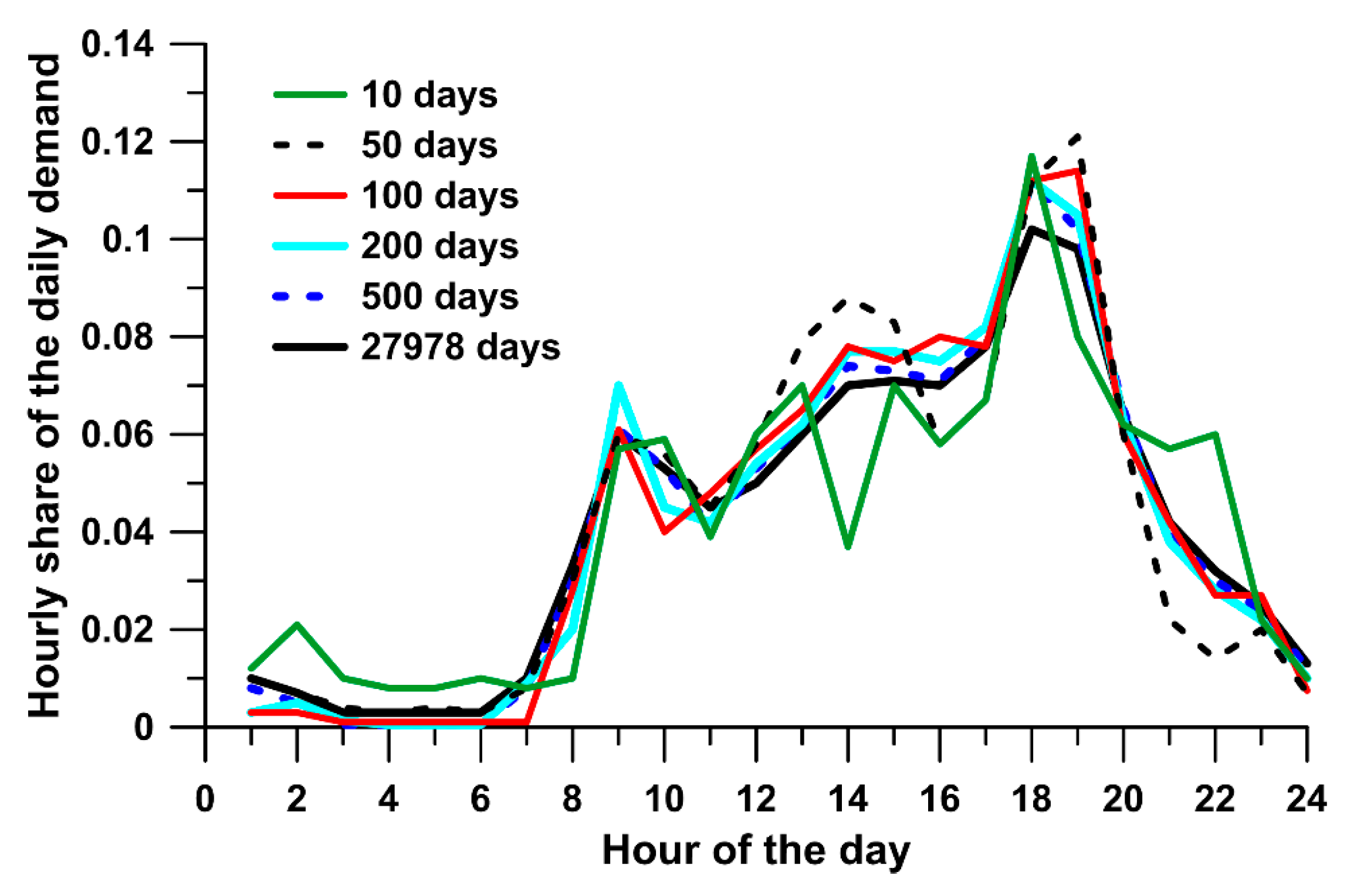
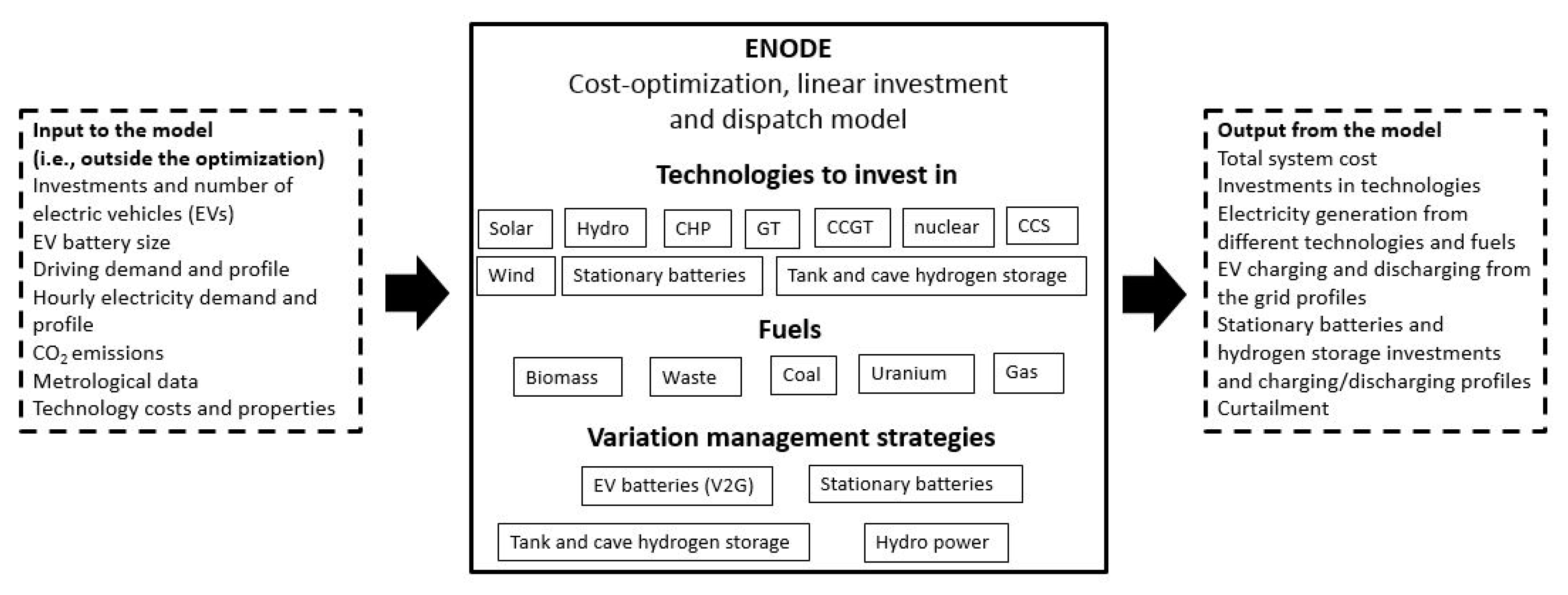
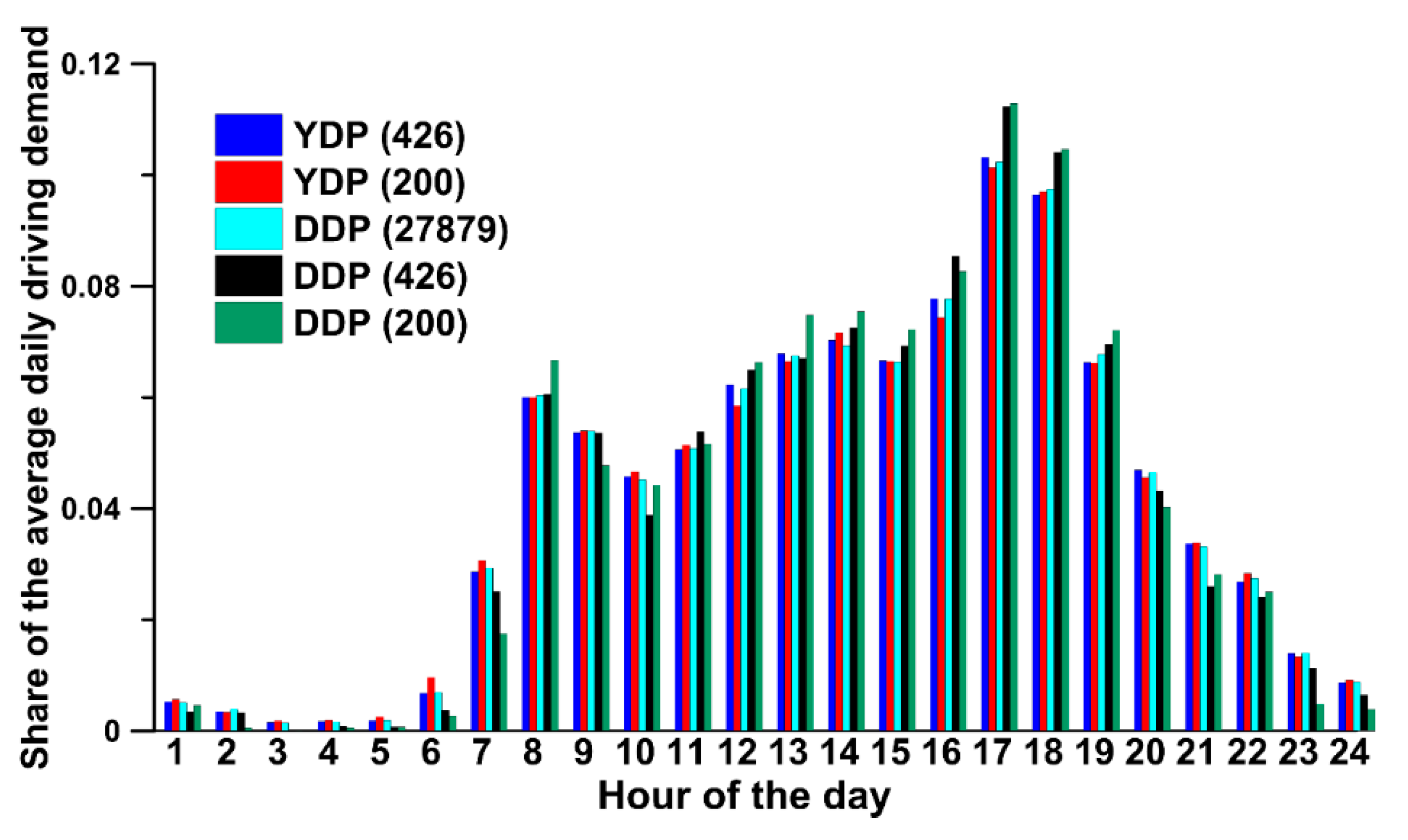
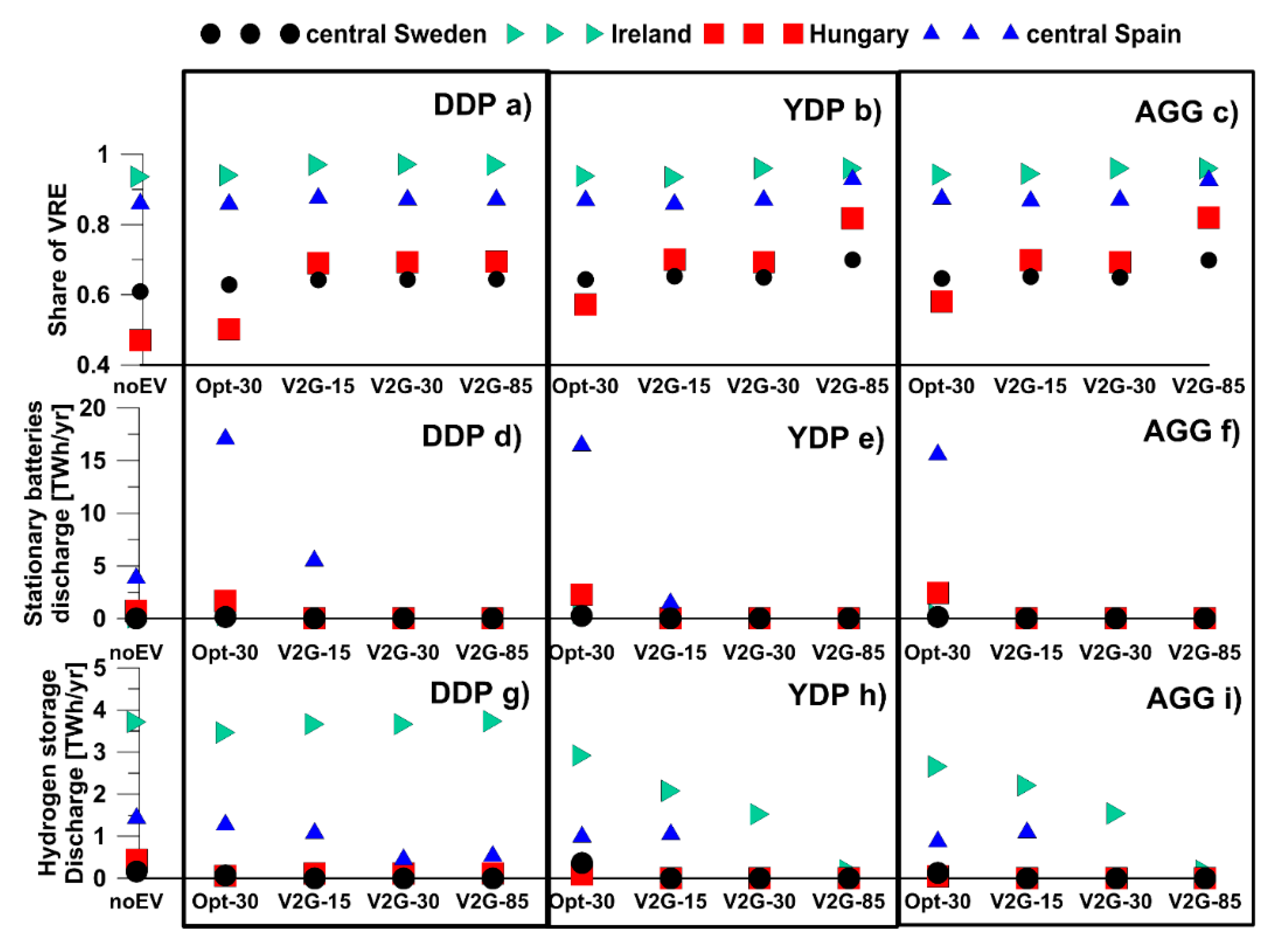
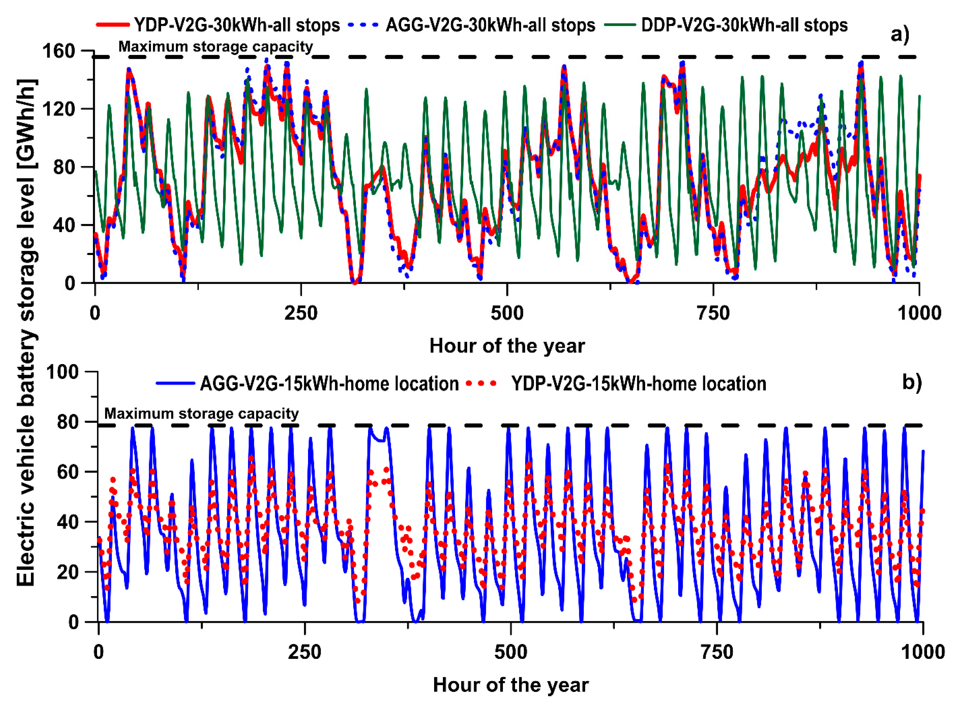
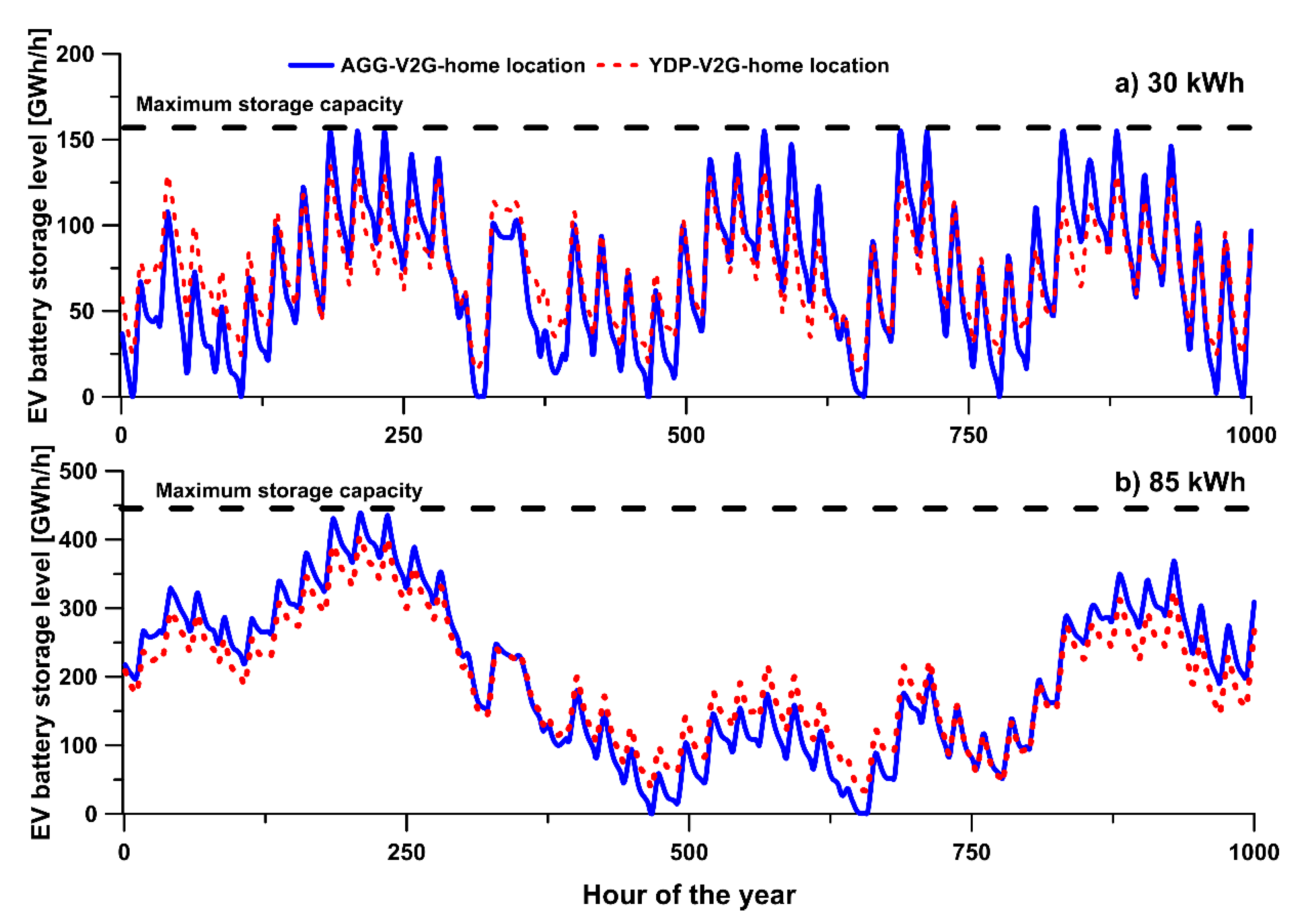
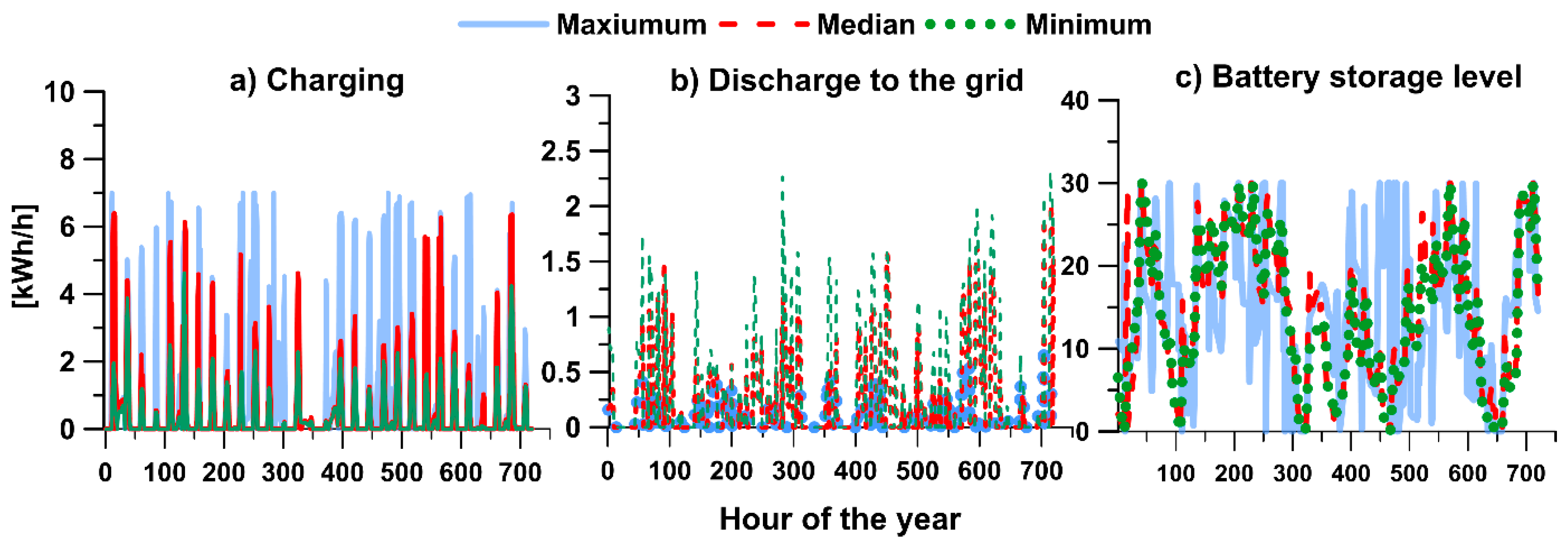
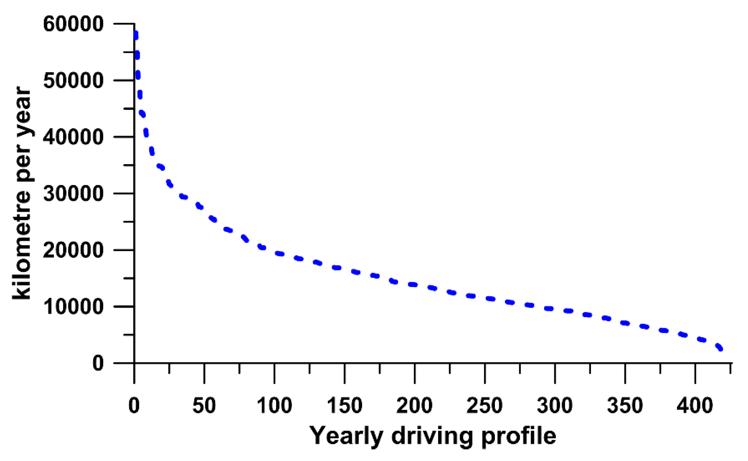
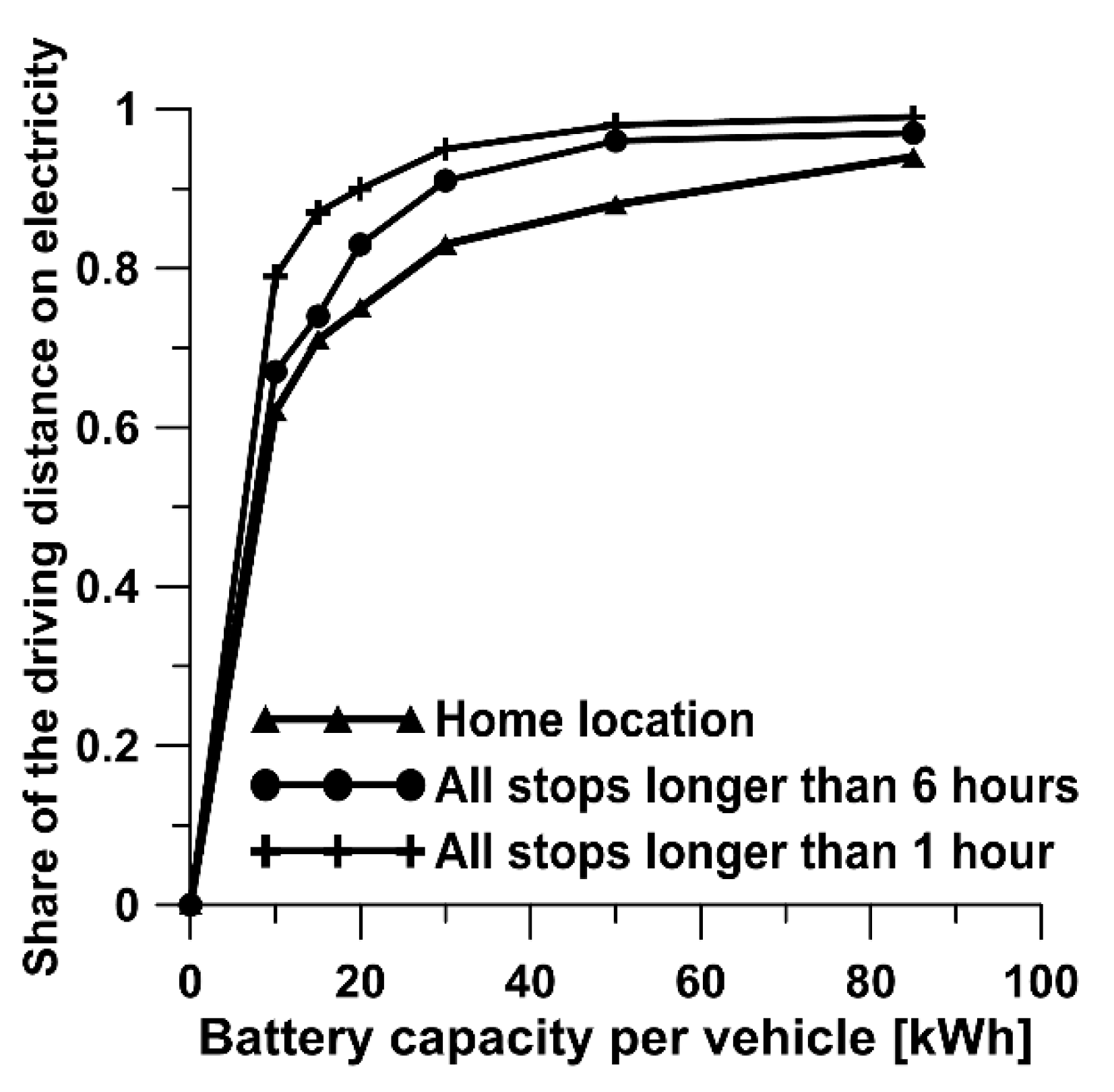
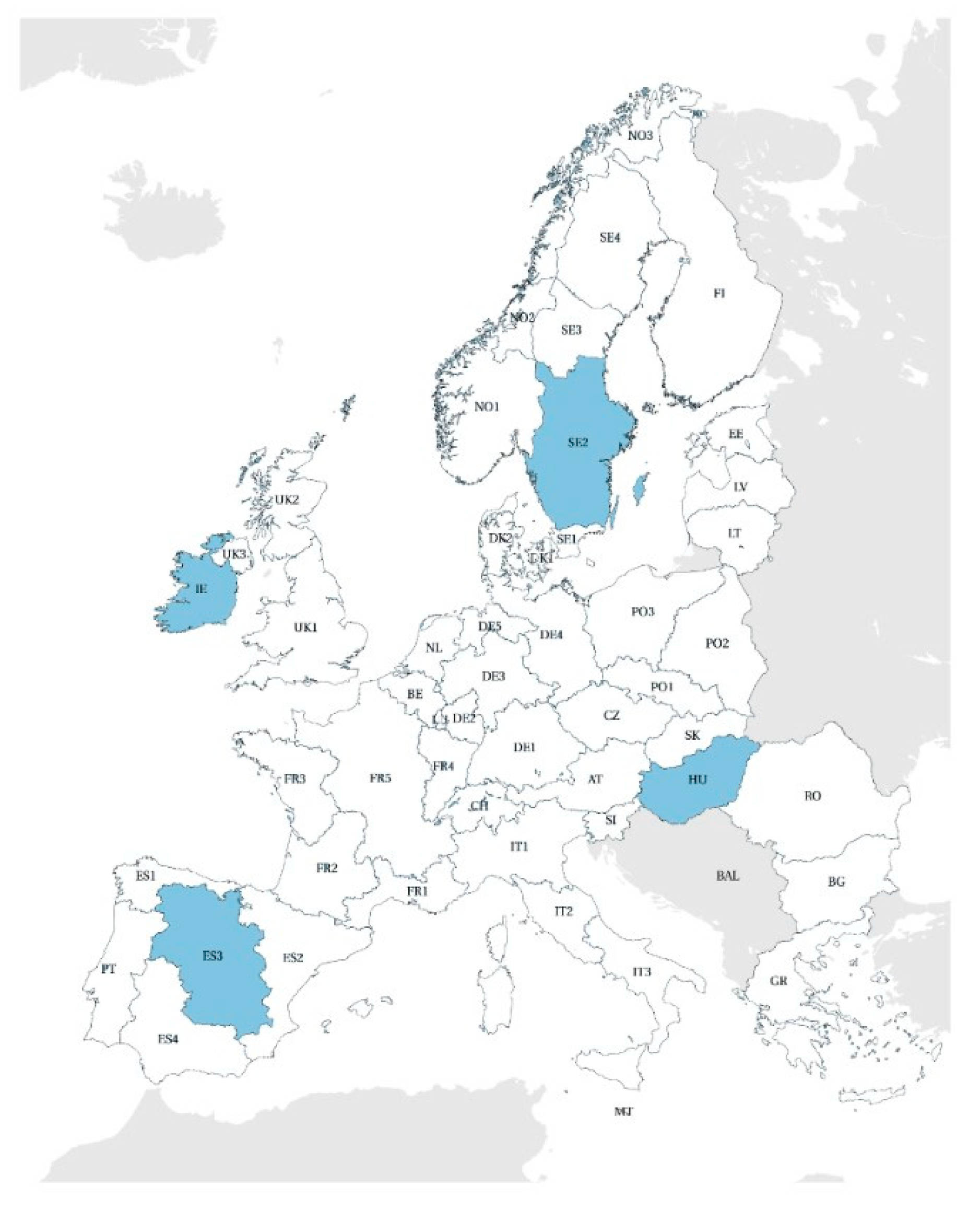


