System-Supporting Operation of Solid-Oxide Electrolysis Stacks

Abstract

Flexible, system-oriented operating strategies are becoming increasingly important in terms of achieving a climate-neutral energy system transformation. Solid-oxide electrolysis (SOEC) can play an important role in the production of green synthesis gas from renewable energy in the future. Therefore, it is important to investigate the extent to which SOEC can be used flexibly and which feedback effects and constraints must be taken into account. In this study, we derived a specific load profile from an energy turnaround scenario that supports the energy system. SOEC short-stacks were operated and we investigated the impact that the load profile has on electrical stack performance and stack degradation as well as the product gas composition by means of Fourier-transform infrared spectroscopy. The stacks could follow the grid-related requirement profiles of secondary control power and minute reserves very well with transition times of less than two minutes per 25% of relative power. Only short-term disturbances of the H₂/CO ratio were observed during transitions due to the adjustment of feed gases. No elevated degradation effects resulting from flexible operation were apparent over 1300 h, although other causes of degradation were present.

1. Introduction

The conversion of electrical energy from renewable sources into certain chemicals, commonly known as Power-to-X (P2X), is conceived as an important building block for de-fossilizing the chemical industry and to increase the flexibility of the electrical grid. Various technical approaches to this are being discussed and high-temperature electrolysis is regarded as a promising future technology. Due to its high efficiency and development potential, it could even be a competitive alternative to current electrolysis technologies (i.e., alkaline- and polymer membrane-based systems) in the future and play an important role in building a GHG-neutral economy [1]. This also applies to high-temperature co-electrolysis (HTCoEL), which is under consideration here for the integrated production of synthesis gas with different stoichiometries.

In the case of co-electrolysis, water and carbon dioxide are simultaneously reduced in a high-temperature solid-oxide electrolysis cell (SOEC) to yield a mixture of hydrogen and carbon monoxide, also known as synthesis gas (syngas). On the fuel side (cathode) of the electrolyzer, the reduction of water takes place according to Equation (1). The reduction of carbon dioxide can follow the pathway of direct electrochemical reduction according to Equation (2) or indirect heterogeneous reaction of H₂ from Equation (1) with CO₂ (Equation (3)) on the catalytically active nickel surfaces of the electrode (also known as the reverse water–gas shift reaction). However, recent reports suggest that in the case of Ni/GDC electrodes, CO is almost fully produced catalytically/thermodynamically via the RWGS reaction and therefore the steam electrolysis reaction (Equation (1)) is totally selective [2]. In any case, oxygen anions described in Equation (1) or (2) migrate through the electrolyte to the air side (anode), where they are oxidized and ultimately yield oxygen.

$$2{\mathrm{H}}_2\mathrm{O}+4{\mathrm{e}}^{-}\rightleftharpoons 2{\mathrm{H}}_2+2{\mathrm{O}}^{2-}$$

(1)

$$2{\mathrm{CO}}_2+4{\mathrm{e}}^{-}\rightleftharpoons 2\mathrm{CO}+2{\mathrm{O}}^{2-}$$

(2)

$${\mathrm{CO}}_2+{\mathrm{H}}_2\rightleftharpoons \mathrm{CO}+{\mathrm{H}}_2\mathrm{O}$$

(3)

$$2{\mathrm{O}}^{2-}\rightleftharpoons {\mathrm{O}}_2+4{\mathrm{e}}^{-}$$

(4)

The produced syngas can be very flexibly used as a feedstock in traditional chemical processes to produce complex chemicals [3,4]. Depending on the operating conditions (foremost among these temperature and feedgas composition), different ratios of H₂ to CO for different upstream processes can be produced. This technology is currently in the laboratory stage (TRL 3–4) in the form of cells, stacks, and a complete system, including auxiliary units and test rigs, and is being continuously further developed. Techno-economic analyses of the co-electrolysis-based synthesis of hydrocarbons show that there is potential for achieving energetic efficiencies of >60% given efficient heat integration [5]. A future target could be the integration of co-electrolysis and direct methanation, and an exergy efficiency of up to 81% using a combined SOEC-methanation reactor with a spatial temperature gradient [6].

An important question in the context of the techno-economic analysis of high temperature co-electrolysis is the definition of interfaces and requirements with respect to system integration. Amongst other things, the aim was to assess the extent to which electrolysis operation can take on system-related functions in power grid operation, i.e., how the flexibility potential of HT co-electrolysis can be assessed. Thus far, the flexibility of HTCoEL has been evaluated fairly cautiously in the literature. Smolinka et al. [7] estimated the sensitivity of the ceramic of an SOEC to the mechanical stresses arising from temperature changes in the stack due to changes in power consumption to be significantly greater than, for example, the polymer membranes in proton exchange membrane electrolyzers (PEMELs). The result could be a reduction in overall lifetime. Nevertheless, this attests to the ability to follow load changes quickly [7,8]. Coupling to fluctuating energy sources is considered possible under the condition that the stack is always kept at an elevated temperature in standby mode and thus especially large temperature fluctuations and corresponding ceramic stresses are avoided [8]. At Aalborg University, a project was carried out in collaboration with Haldor Topsoe to improve the SOEC technology for system-oriented use in future energy systems with a high proportion of fluctuating, renewable energy [9]. It was demonstrated that large SOEC stacks can also be operated for grid balancing in Denmark. However, no specific statements were made with respect to degradation effects. Recently, the simulation of dynamic co-electrolysis operation for tracking scaled wind power input using a 3D stack model was shown and a control strategy evaluated for stabilizing the stack temperature profile during load transitions [10].

Essentially, the question of the flexibility potential can be addressed from two different perspectives: On the one hand, the flexibility requirements can be formulated from a system perspective and the reaction options of the process compared. Another approach is to first define the flexibility properties from a process perspective and then to assess them for their compatibility with the system’s flexibility requirements. This paper describes the development of a requirement profile for a degradation test with a flexible operation style for an SOEC stack in laboratory applications. For this, the requirements are first derived from a system perspective. The specific properties of the test stand are then directly incorporated into the formulation of the requirement profile. Other working steps, such as a detailed description of the flexibility options of the SOEC stack also in the context of its system embedding, and which were carried out to estimate the flexibility potential, are not the subject of this paper.

2. Experimental Procedure

2.1. Stack and Cell Design

We employed three four-layer stacks of the Jülich F10 design [11] in this study. This design contains one anode-supported cell in fuel cell mode (ASC) per layer, yielding a total active area of 80 cm². The details of the cells with the layer sequence and their respective thicknesses are given in

Table 1. Cell and stack components of a repeating unit.

Component	Thickness	Material
substrate	~300 µm	Ni/8YSZ
fuel electrode	7 µm	Ni/8YSZ
electrolyte	10 µm	8YSZ
barrier layer	2 µm	CGO (Ce0.8Gd0.2O1.9)
air electrode	20 µm	LSCF (La0.58Sr0.4Co0.2Fe0.8O${}_{3-\delta }$)
air-side contact layer	140 µm	LCC10 (LaMn0.45Co0.35Cu0.2O3)
protective layer	~50 µm	MCF (MnCo1.9Fe0.1O4)
interconnector	2.5 mm	Crofer 22 APU

, which also states the contact layers and the protective coatings of the interconnects (IC), as well as their thicknesses. The cells were produced by CeramTec (Plochingen, Germany). The cerium-doped gadolinium oxide (CGO) barrier layer was screen-printed and the protective coating at the interconnects was prepared by means of atmospheric plasma spraying. The electrical contact between the IC and substrate was achieved by nickel meshes. The sealing inside the stack was ensured by glass-ceramic on all bonding surfaces and the external sealing by flat mica gaskets. Detailed descriptions of the cell and stack design and assembly can be found in [12,13,14,15]. The stack temperatures were monitored by nine thermocouples inserted about 40 mm-deep into the stack. In the following, the sensor at the center of the stack between layers 2 and 3 and in the middle between the gas entry and exit is designated as the stack temperature (T_Stack). Joining of the stack was performed for 100 h at 850 °C in the furnace with a load of 100 kg. The reduction of the substrate and fuel electrode was performed at 800 °C in an H₂/Ar mixture with stepwise increasing hydrogen concentrations between 9% and 62% H₂.

2.2. Gas Analysis

In order to determine the concentrations in the product gases, we employed a mobile gas analysis system consisting of a Fourier-transform infrared spectrometer (FTIR; CX4000, Gasmet, Helsinki, Finland) for IR-active gases and a thermal conductivity detector (TCD; Conthos-3, LFE GmbH, Bruchköbel, Germany) for hydrogen. The interference error caused by CO₂ and CH₄ in the TCD was thus compensated. The complete system, including the sampling system a described elsewhere [16]. Although the gas analysis system supports the measuring of hot gases, including steam, the test rig offered only a sampling port after the exhaust cooler. Therefore all gas analyses presented here were performed with dry gases (i.e., CO₂, CO, H₂, and CH₄). For the gas analyses, a third stack identical in construction was utilized.

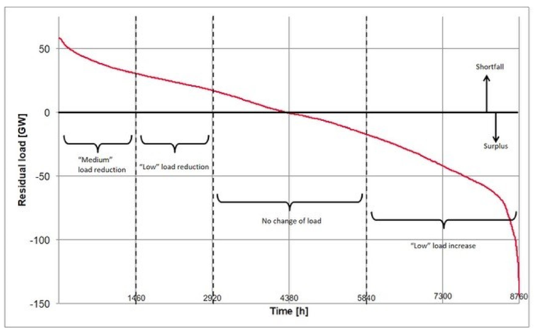
2.3. Load Profile Development for Flexibility Assessment

With an increasing share of renewable energy in power generation, flexibility in the power system is becoming ever more important to balance out fluctuations in power generation and to ensure the supply of electricity at all times. By definition, the use of flexibilities is “the modification of generation injection and/or consumption patterns in reaction to an external signal (price signal or activation) in order to provide a service within the energy system.” ([17], p. 6). There are two types of flexibility: network-related (grid-related) and system-related services, each of which has different flexibility requirements.

Grid-related flexibilities are concrete system services that are actively requested and used by grid operators to stabilize the electricity grid and ensure its safe operation. This includes in particular the provision of balancing services, the requirements of which are precisely defined in the respective regulatory and technical guidelines (prequalification procedures) for participation in the three balancing energy markets in Germany. These requirements serve as a starting point to check the test stack for the provision of already relevant performance gradients and response times. For this purpose, sample protocols of the prequalification procedures taken from [18] for participation in the control energy market are simulated. It is shown that the response times and performance gradients for flexibility in the secondary control power product classes (activation time ≤5 min and performance time of ≤10 min) and the minute reserve for the test stack in the laboratory do not cause any difficulties from a purely technical point of view. The requirements of the primary control power are not tested, as this is not considered useful for electrolyzers due to the very frequent short-term clock cycles (≤30 s) in direct dependence on the target frequency (50 ± 0.01 Hz).

Therefore, the focus of further investigations is on the system-supporting requirements for flexibilities, on the basis of which a stabilization of the entire electrical energy system during the transformation to a completely renewable power system (energy transition) is pursued. This includes, in particular, the best possible adaptation of electricity demand and generation with the aim of minimizing residual load, i.e., load minus renewable generation. In order to be able to realize the further increasing share of volatile power generation in the system in the context of the sustainable energy turnaround, future consumers must behave as compatibly with the system as possible, making use of technologies such as electrolysis as a link in the so-called sector coupling. The system-related requirements for the possible applications of flexibilities are much more diverse than in the grid-related case, and can vary greatly, depending on the energy system’s composition. Aside from the reaction times (see above) as well as the amount and rate of load changes, these are mainly determined by the necessary application or availability time. From the point of view of the electricity system, this is the time over which an amount of energy can be shifted or a load changed. This maximum period of time over which flexibility can be made available determines its application potential with respect to the balancing of fluctuations in renewable power generation, which can range from hourly, to daytime varying patterns, especially in case of PV power feed-in, to extensive load reductions over days (“dark wind lull”).

In order to illustrate the system-related application possibilities of the high-temperature laboratory stack under consideration and to determine the potentially resulting reaction effects on the service life of the stack and the qualities of the product gas, a specific system-serving requirement profile is derived on the basis of a certain scenario. This scenario was developed by the Technical University of Munich (TUM) as part of the Kopernikus P2X joint project (Phase 1) and made available for our analyses. It is a simplified scenario that describes Germany in accordance with the “Climate Protection Scenario 2050” (Öko-Institut/FhG-ISI) [19] with and without the use of Power-to-X technologies and aims to reduce annual greenhouse gas emissions by at least 80% by 2050. In the reference scenario without Power-to-X, the fluctuating renewable share of gross electricity generation is approximately 78% ([20], pp. 57–61). The residual load curve (the difference between electricity demand and renewable electricity feed-in) in terms of hourly resolution for the year 2050 in Germany is derived from this scenario and is used as a basis for the development of the system relevant requirement profile. The course of the residual load is an important indication of the possible requirement profiles of flexibility demand in a future energy system with a high proportion of fluctuating producers. The resulting annual duration curve of the residual load of the reference scenario is shown in Figure 1. The positive residual load (left-hand side) reflects the remaining demand for electricity before the implementation of the flexibilities, whereas the negative residual load (right-hand side) indicates the corresponding surplus in the system. It is easy to see that there is a surplus and shortfall of about half of the hours of a year. Overall, the entire electricity demand can be covered by renewable electricity generation (on the balance sheet), with a slight annual balance surplus of about 37 TWh.

The technical specifications of the laboratory stack used for the degradation test embody various premises that must be taken into account in the development of the requirement profile.

• The requirement profile should initially consist of fairly “flat” and short-term cycles that do not exceed the exothermic operating spectrum of the stack. Two different stages of load reduction (up to 50% or 75% of the nominal load) and one stage of the load increase (up to 125% of the nominal load) in addition to standard operation (100% nominal load) are defined as load change modes that are likely to be feasible but are challenging.
• The operational management of the stack under investigation also makes it necessary to use cyclically recurring requirement profiles for the degradation test. For this reason, a representative weekly profile (to be used as often as possible in the context of the system requirements) was developed, and was then strung together for the test over several thousand hours.
• As the performance gradients of the secondary control power product class are demonstrably feasible for the test stack, they are also used for the load change rate in the degradation test.

For the development of an initial, comparatively flat requirement profile, two load reduction and one load increase stages must be considered on the side of the stack, which differ from normal operation (no load change). In order to determine the thresholds for calling up the stages, the residual load is divided into segment areas according to the annual hours (see Figure 1).

(1) The first third of the annual duration line summarizes the hours of moderate to severe under-coverage in the system; in this example it corresponds to residual loads of >17.1 GW. During these hours, different levels of load reduction are required due to the deficit: For half of the hours (i.e., 1/6 of the year) a high level of load reduction (up to 50% of the nominal load) is triggered in the case of high deficits (>30.5 GW) and for the other half, i.e., in the case of deficits between 17.1 GW and 30.5 GW, a lower level of load reduction (up to 75% of the nominal load) is triggered. (2) The second third of the annual hours is categorized by situations with relatively low under- or over-coverage (between 17.1 GW and −17.1 GW). As the flexibility of the HTCoEL is comparatively costly, no load change is assumed for these situations, with probably fairly low flexibility requirements from the point of view of the electrical energy system. At the same time, it is assumed that within this range, there will be cheaper alternatives in the set of flexibility options, which will be used preferentially. (3) The last third with cover situations of <−17.1 GW will, in turn, allow a moderate load increase corresponding to the potential of the stack in this test of 125% of the nominal load.

Next, using the categorization of system-related applications described above, the seasonal progression of the residual load curve was evaluated in order to identify a typical week with a high proportion of recurring and short-term usage cycles. Such a course was particularly favored by a high share of solar electricity, which is characterized by high daily fluctuations and corresponding daily application situations lasting several hours. Such daily fluctuations are less frequent in winter, however, when over- and under-cover situations lasting several days alternate, which are characterized in particular by the occurrence of windy phases with high and low wind speeds. These are less suitable as indicators of load changes in degradation tests. Therefore, a summer week was selected for the system-relevant requirement profile. Thus, the duration and frequency of under- and over-cover situations were determined, which were assigned to the four deployment categories derived above. For each category, the relative deviation from the weekly average of the summer weeks was determined and the week that came closest to this average selected. The result was that week 27 of the reference scenario year of 2050 best fulfills these conditions, had all four deployment categories relatively often, each with common durations, and was therefore used as a system relevant requirement profile as shown in Figure 2, for the test of the SOEC lab stack.

2.4. Stack Operation

The feed gas for the stack during long-term co-electrolysis operation was a mixture containing 60% H₂O, 30% CO₂, and 10% H₂ that produced a product gas with an H₂O/CO₂ ratio of 2.05–2.15. Technical grade hydrogen and CO₂ (99.7%) were supplied with mass-flow controllers (MFCs). Any volumes used in the following are given at a standard reference temperature of 273.15 K and a pressure of 101,325 Pa. Electrical once-through steam generators were employed for supplying the steam. The feed-water was introduced by a diaphragm pump (stack A) and the flow rate was calibrated gravimetrically (offline) and using a high-pressure dosing pump with two pistons (stack B). On the air-side, we used an air flow rate of 2 L min⁻¹ oil-free compressed air (dew point <−60 °C), which was sufficient to flush the generated oxygen from the cell, but maintained a low differential pressure across the electrolyte.

The stacks were operated galvanostatically at 800 °C in counter-flow mode. We opted to operate the stacks in constant-current mode to keep the conversion ratio of the stack constant for a given power level. Due to limitations in the test rig the feed gas flow rate was constant for stack A, but stack B was operated with a constant conversion ratio of 70% (i.e., dynamic feed gas flows). The current densities for the different power levels were derived as follows (example values for stack B): First the maximum current density during continuous operation was chosen (0.7 A cm${}^{-2}$). The stack power needed to sustain this current density with the feed gas mixture given above, at 800 °C, and a conversion ratio of 70% at the beginning of the load-cycle experiments was defined as 125% relative stack power (e.g., −264 W). The other power levels were defined relative to this level (e.g., −211 W corresponded to 100% relative power). To determine the current density for each relative power level, a characteristic P–j curve of the stack was measured and then taken into account (e.g., −0.7 A cm${}^{-2}$ at −264 W corresponded to 125% relative stack power and −0.57 A cm${}^{-2}$ at −211 W corresponded to 100% relative stack power). The P–j curve of stack B was measured at constant 70% conversion ratio, the one for stack A at a constant feed gas flow rate suitable for 70% conversion ratio at the maximum current density. The employed conversion ratio of 70% was regarded as being the lower end of a commercially relevant window.

For choosing the maximum current density, two main constraints were considered. The mass flow controllers and the steam generator had to support the flow rates for the highest and lowest power level. The mass flow controller for hydrogen defined the lowest possible total feed gas flow rate and the steam generator defined the largest possible total feed gas flow rate. As the second constraint, we also intended to keep all layer voltages during the experiments at or below the thermoneutral voltage to avoid a transition between the two operating regimes (endothermal vs. exothermal) mid-experiment. Therefore the current density of the highest power level was chosen in a way that the resulting voltages at the given feed gas composition, 70% conversion ratio, and stack temperature of 800 °C did not exceed 1.35 V (U_th calculated to 1.344 V). Additionally, we planned to have a large voltage reserve allowing for a pronounced degradation of the cells during the experiment.

During electrolysis operation, the resistance of the stack was measured by applying a small rectangular current modulation (2 A) to the DC current (known as the “linear polarization resistance” method). This was repeated for 30–50 cycles every 6–8 h.

In the case of the load cycles with a static gas supply, the electrical current was switched without a ramp as fast as the power supply unit could manage it, which could be expected to be within a few tens of milliseconds. In the case of the load cycles with a dynamic gas supply, the current was adjusted with a ramp of 60 A cm ${}^{-2}$min${}^{-1}$, roughly corresponding to a change in the relative power of 133 min${}^{-1}$. The steam was changed with a rate of 1.63 L min${}^{-2}$. The steam generator (SG) had the highest latency, which was tested to be between 30 s and 60 s. The SG also had the slowest rate-of-change, and therefore the other gases were changed with a matching ramp to finish their ramp at the same time as the SG. To account for the latency, the carbon dioxide increase (in the case of load increases) always followed with a 60 s delay after starting a ramp for the SG to prevent any potentially unsafe reductions in the H₂O/CO₂ ratio. This ratio (which also determines the ratio of oxygen/carbon in the feed) is important to prevent any soot formation in the pipes and components of the test rig and the stack. Therefore, our intention was, that during transitions of power levels, the H₂O/CO₂ ratio may shortly increase but never decrease. Finally, the current change ramp was started. In the case of load reductions, the ramps for the current, steam, and carbon dioxide were started simultaneously and that for the hydrogen reduction followed in order to always maintain hydrogen concentrations of >=5% in the feed gas mixture.

The load cycles were accelerated by a factor of 5 in order to accelerate testing and increase the number of load changes, i.e., the derived representative week long sequence of required relative stack power was performed in 1.4 days.

3. Results and Discussion

Several phases of stationary and dynamic operation at three short stacks were evaluated for this study.

Table 2. Operational phases.

Stack	Phase	Description	j	CR	Duration	Degradation
						U	R
			A cm${}^{-\mathbf{2}}$	%	h	mVkh${}^{-\mathbf{1}}$	m$\Omega$cm${}^{\mathbf{2}}$kh${}^{-\mathbf{1}}$
Stack A	A1	Load cycles S	0.71	75	552	31	44
Stack A	A2	Load cycles S	0.71	70	336	37	52
Stack A	A3	Load cycles S	0.71	70	264	36	50
Stack A	A4	Stationary	0.60	70	360	8	14
Stack A	A5	Stationary	0.71	70	397	18	25
Stack B	B1	Stationary	0.70	70	239	62	89
Stack B	B2	Stationary	0.70	60	297	46	66
Stack B	B3	Stationary	0.70	50	129	43	62
Stack B	B4	Stationary	0.70	70	86	64	91
Stack B	B5	Stationary	0.70	70	96	55	79
Stack B	B6	Load cycles D	0.70	70	1323	14	20

gives an overview of these and summarizes the observed degradation rates. Values for j are given for the 125% power level of the load-cycle operations and in case of phases with static gas supply (A1, A2, and A3) the values for CR are also given for the 125% power level. The degradation rates given for stack A exclude data for layer 4. For stack B, no layer was excluded. Further details will be discussed below.

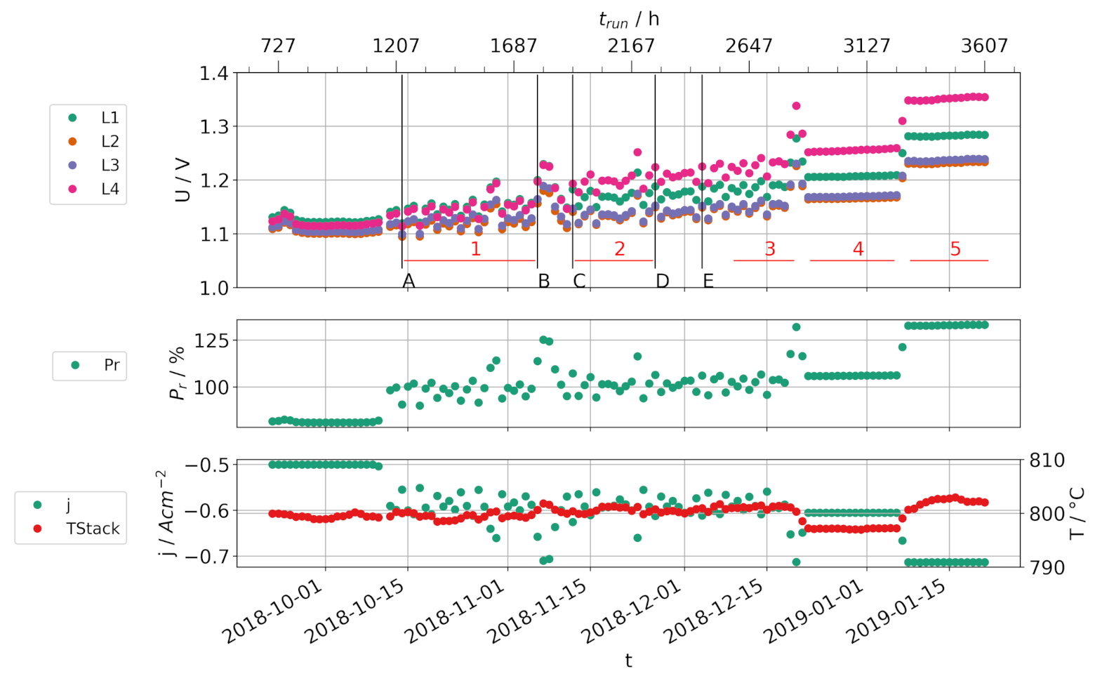
3.1. Load Cycles with Static Gas Supply

The first stack experiment varied the current density at stack A according to the requested load profile, but limitations in the test rig necessitated keeping the feed gas flow rate constant. Thus, the conversion ratio was different for each load level, with 70% net conversion at the 125% relative power level and 34% at the 50% level.

About 1500 h of load cycles were performed in this manner. Then, 1152 h in three distinct phases (A1, A2 and A3) were evaluated to estimate the degradation rate during this type of stack operation. Figure 3 shows the timeplot of the individual layer voltages with daily averaged values for the experiment with stack A. We also show the instantaneous cell resistances at the operation point measured by the linear polarization resistance (LPR) method in Figure 4. This parameter reacts with substantial sensitivity to changes in operating conditions and state-of-health and enables us to clearly distinguish different operational phases and discrete damaging events. These are characterized by sudden and strong increases in the cell resistances. We identified specific changes in the operational parameters that coincided with these sudden increases in the resistances. These changes are shown in

Table 3. Events at stack A.

Event	Description
A	Begin load cycle operation
B	Replacement of water pump + recalibration
C	conversion ratio 80% for  30 min
D	Increase of steam generator temperature to 510 °C
E	Increase of steam generator temperature to 520 °C

. We believe that these caused a significant degradation in the cell performances. Furthermore, as these events were exceptional and are not related to the load cycle operation, we determined the given degradation rates during the three phases of stable operation without damaging events.

At the end of phase A1, we measured the steam concentration in the feed gas by FTIR and concluded that the amount of steam was lower than intended, which increased the net conversion ratio during phase A1 from the intended 70% to 75%. The pump for the feed-water was replaced and calibrated to correct the amount of steam for the remainder of the experiment. Between phases A1 and A2, no load-cycles took place, because we performed a stack characterization with measurements of the product gases under different conditions. In addition, during the night, the stack was kept on dry standby in pure H₂. Therefore, the daily averaged cell voltages were increased for 3–4 days, because they included periods of open-circuit voltages. Directly before entering phase A2, we performed a short operation at higher conversion (80%) and noticed a rapid increase in the cell voltage of layer 4. This was also reflected by the increased resistances after we resumed normal load-cycle operation. The other cells showed a small decrease in performance. While we have no direct proof of what actually took place, we suspect a local starvation of steam in parts of the cell. This is supported by an observation made during the post-mortem analysis, where we found a partial delamination between the electrolyte and Ni/YSZ electrode near the gas-exit side. This delamination was the largest for layer 4, followed by 1, and quite small for 2 and 3. As a result of this event, we excluded layer 4 from the determination of the average degradation rates given in Table 2.

Events D and E between phases A2 and A3 were both an increase in the operating temperature of the steam generator, and were both followed by a significant increase in cell resistances for several days. We think it is likely that this led to a volatilization of poisoning substances from the feed-water or steam generator itself. Investigations of this effect are underway and their results will be reported soon, but are unfortunately beyond the scope of this publication.

The general upward trend of the relative power observable in Figure 3 and Figure 4 also reflects the cell degradation, because increased power is needed to sustain the current. Overall, the degradation rates during the load cycles with static gas supply were fairly consistent over the three distinct operational phases. Unfortunately, they were on a fairly high level of 5.5% kh${}^{-1}$ to 6.3% kh${}^{-1}$ relative to the initial cell resistances and 2.5% kh${}^{-1}$ to 3% kh${}^{-1}$ relative to the initial cell voltages.

3.2. Load Cycles with a Dynamic Gas Supply

We then performed an improved stack experiment and varied the current density at stack B according to the requested load profile and automatically adjusted the feed gases accordingly in order to keep the net conversion constant at 70% for each power level. Figure 5 shows an example of one accelerated sequence in stack B with a dynamic feed gas supply and a constant conversion ratio of 70%. The measured profile corresponds to the requested profile from Figure 2 very well. There are only very minor and short-term overshoots in the relative power that are caused by the lagging adjustment of feed gases.

The stack temperature changes for the entire profile remained below 2 K. Given a thermoneutral voltage of 1.344 V for the given gas mixture, the heat consumption at the 125% power level is estimated to about 32 W for the complete stack. The lower power levels had lower layer voltages (i.e., larger difference to the thermoneutral voltage) and therefore larger heat demand per mole converted gas. They also had lower currents. The heat demands are estimated to 36 W (100%), 35 W (75%), and 29 W (50%) for the other power levels. This explains why the stack temperature is lowest (and nearly the same) for the 100% and 75% levels and highest (and also nearly the same) for the 125% and 50% levels. The maximum difference in heat demand is 7 W. Taking into account the small stack size and good thermal conductivity within the stack, this is the reason for the small difference in stack temperature. While it was not a primary constraint of the power profile, this shows that it is possible to build the power profile in a way that not only suits the energy system, but also maintains a flat temperature profile that minimizes mechanical stresses.

A total of 1323 h of load cycles were performed in this manner and evaluated to estimate the degradation during this type of stack operation. Figure 6 shows a time plot of the individual layer voltages with daily-averaged values for the experiment with stack B. We also show the instantaneous cell resistances at the operating point measured by the LPR method in Figure 7.

No discrete damaging events occurred during this experiment. The overall degradation was fairly constant during the experiment and amounted on average to 20 $\Omega$ cm${}^2$ kh${}^{-1}$ (3.6% kh${}^{-1}$) and 14 mVkh${}^{-1}$ (1.2% kh${}^{-1}$). This is strikingly less than we observed above for the load-cycles with a static gas supply and also less than during the stationary operation of both stacks. We regard this as a clear indication that a dynamic stack operation that supports an electrical grid does not cause increased degradation rates in the stack during co-electrolysis.

We found it difficult to accept that the dynamic gas supply is the deciding factor in this much reduced degradation rate in comparison to the load-cycles with a static gas supply. A common degradation phenomenon in Ni/YSZ electrodes is the loss of active nickel from the functional layer of the electrode. This effect is, in our experience, most pronounced in the first ~2–3 kh of operating hours and often the dominating component in the overall degradation. When most of the finer nickel particles in the vicinity of the electrode have migrated away, the degradation rates drop. We performed the load cycle operation at stack A rather at the beginning of the stack’s life, at between 1200 h and 2700 h. For stack B, the experiment was performed at between 3330 h and 4660 h. This may place both experiments in a different intrinsic degradation regime. In this case, a direct comparison is difficult. Unfortunately, this is a common problem for experiments on real stacks. Moreover, the discrete damaging events at stack A, especially the suspected introduction of poisoning substances, probably had some long-term impacts as well.

Another potential cause for increased degradation may have been the speed of current changes, which was performed much faster on stack A than stack B, as no gases had to be adjusted. An issue could have been significant overshoots in the galvanostatic control loop, but the current steps were limited in magnitude (to roughly 0.125 A cm${}^{-2}$), which makes this unlikely in our setup. Moreover, temperature changes, which in theory could induce thermal strains, were minor (<2 K) for the current steps used. Sufficient amounts of reactants were always available, and so no starvation upon fast current switches could be expected. In summary, we could not fully rule out this possibility at the moment, but we regard it as remote.

Figure 8 shows an accompanying analysis of the product gases for several load transitions between the load levels, as well as the electrical parameters and feed gas flows. It does not show a complete profile, but the applied load levels and transitions were precisely reproduced. During power reductions, the current reduction ramp starts and then the feed gases follow a few seconds later with a corresponding ramp. During power increases, the feed gas flows start their ramp-up first, and shortly after the current ramp-up with the corresponding speed is initiated. In addition, the ramp-up for the steam is always initiated slightly in advance of the other gases in order to take the latency of the steam generator into account. In both cases, this led to a short reduction in the conversion ratio and a short disturbance in the H₂/CO ratio in the product gas which could clearly be seen. Moreover, the measured concentrations follow the change in operating conditions with about a 60 s delay, which is determined by the dead volume between the stack and FTIR spectrometer. An additional dead time of 30 s exists between the gases measured by FTIR and H₂ and these two effects correspond to a phase shift and cause a dispersion in the observed peaks in the measured concentration and especially the H₂/CO ratio.

As expected, for constant loads, the product gas concentrations for the different load levels are nearly the same and the H₂/CO ratios are very similar. Deviations in this ratio could interfere with up-stream processes. During load transitions, such short-term deviations are difficult to avoid because of the latency and limited rate-of-change of the feed gas supply. In this respect, the most critical BOP equipment is the steam generator whereas the mass flow controllers react more quickly. The change in the electrical parameters of the stack took about 6 s to achieve a 25% load level change, and the adjustment of gases took about 80 s. Not surprisingly, short-term (about 2 min) disturbances between 2.1 and 2.8 were clearly observed in this experiment. For load reductions, the flows of steam and CO₂ and electrical current were reduced simultaneously, but for increases, the steam flow was first increased to always ensure safe H₂O/CO₂ ratios in the feed. Therefore, the deviations were usually smaller for load reductions. However, given the short time to restabilization, we considered them relatively minor and the transitions could still be optimized in a well-known system. Moreover, the gas transfer between the stack and any up-stream process can likely be designed in a suitable way to level out these changes in concentrations (e.g., with a buffer vessel). Our assumption is that load changes in the stack as performed here were unlikely to be a serious problem for an upstream process, as only a few per day occurred.

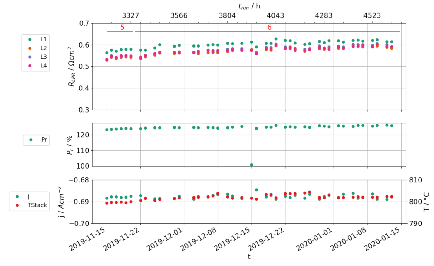
3.3. Stationary Electrolysis

To compare both variants of the load-cycle operation with the degradation rates during stationary operation, we performed phases of stationary operation with both stacks.

In stack A, two periods (A4 and A5) with differing current densities were conducted after the load-cycle operation (shown in Figure 3 and Figure 4, refer also to Table 2). A4 corresponded to the 100% and A5 to the 125% power levels of the load profiles used for the load-cycle operation, and both showed a reduced degradation rate. With stack B, we executed several phases of stationary electrolysis that varied in conversion ratio, but all had the same current density (shown in Figure 9 and Figure 10). Phases B1 and B4 corresponded to the 125% power level. In all cases, very large degradation rates were observed. In particular, they were significantly larger than those determined for all load-cycle experiments. As we already pointed out above, the degradation rates early on in stack experiments are often higher than in later phases of operation, and so this observation was borne out. Independent of the type of operation, the highest degradation rates occur early in the stack’s life, i.e., with the measured rates more influenced than the stationary or dynamic operation.

The direct comparison of A4 and A5 suggests that an increased current density clearly impacts the durability; however, it cannot be determined if it is caused by only the j or the accompanied increase in the cell voltages. In this experiment, the voltages increased well above the thermo-neutral levels, as the stack was near the end of its useful life.

When comparing B1 to B4, there is a clear dependency of the degradation rates on the conversion rates. Our experimental findings until now did not suggest a significant influence of the conversion rate on the degradation rate, unless the conversion rate were to become very high. However, these were mainly undertaken with steam electrolysis. We emphasize here that the step from 70% to 60% had a large impact, whereas further reductions do not change as much. The observed higher degradation at higher conversion ratios also fits the event C in stack A (see Table 3). In the feed gas we used, the convertible gases were 66% H₂O and 34% CO₂. This means that, at a conversion ratio of about 60% or lower, the electrolysis current could only be sustained by steam conversion, which is thermodynamically favorable. At higher conversion rates, at least some CO₂ must also be converted. It is currently accepted that, in the case of co-electrolysis, most CO₂ is converted by the reverse water-gas shift reaction (reaction (3)) instead of direct electrochemical conversion (reaction (2)). The speed of this reaction in regenerating water from CO₂ and H₂ (which can then be electrolyzed again) is finite and takes place on the same nickel surfaces as the electron transfer reactions. In particular, at high conversion rates this likely causes competition by both reactions for the same surfaces of the functional layer. Therefore, it seems highly possible that local conditions with relatively high CO₂ and H₂ and very low H₂O concentrations can be formed. Reference [2] recently reported that a high coverage of adsorbed H₂ could inhibit the dissociative CO₂ adsorption, which is part of the direct electrochemical reduction pathway, and thus would decrease the intrinsic catalytic activity for CO production. In any case, the direct CO₂ reduction pathway anyway requires higher potentials for sustaining the same current. This effect could in addition lead to a kind of local pseudo-starvation and also increase local potentials, perhaps up to damaging levels. Even if the current flow shifts to other cell areas, gas mixtures with very low water activity might promote carbon deposition, which can then damage the microstructure. Some time ago, we observed that the concentration of methane in the product gas rises above the values expected in thermodynamic equilibrium at high conversion ratios, suggesting a change in the reaction mechanism [16]. This may also relate to direct CO₂ reduction at higher potentials and the formation of side products. We intend to follow up this observation with further experiments at high conversion ratios, including dedicated product gas analyses.

3.4. Limitations

Compared to the flexibly operable SOEC laboratory stack, the flexibility is expected to decrease when the stack is embedded in future applications. This is in particular due to additional non-electrical components in the gas and thermal management (especially steam generators and heat exchangers). An extension of the considered system boundaries from the stack in the laboratory environment to the overall system of an HTCoEL leads to new aspects that have to be taken into account when considering flexibility. In this respect, the following requirements and obstacles can be derived, which will have to be analyzed further in the future:

• In the context of the system’s overall embedding, the guarantee of a continuous feed supply to the SOEC and its thermal management represents a major obstacle to flexibility. Even without the goal of flexibilization, these aspects represent very sensitive parameters in the system’s design.
• As the HTCoEL takes place at very high temperatures, sophisticated heat management is essential for its operation. In order to enable the flexible operation of HTCoEL, additional heating capacities or buffer storage tanks, for example, must be taken into account in the design of the heat integration mechanism. This may lead to a loss of efficiency and an increase in system costs.
• Consideration of a flexible mode of operation in the design also means an increase in investment costs for other components. For example, conventionally used compressors are not designed for many load changes, and so higher quality compressors must be used.

4. Conclusions

SOECs can be flexibly operated with consideration to process-technical conditions and provide system services. For this purpose, two different requirements with different objectives must be distinguished: grid-related ones to stabilize grid operation and system-related ones to stabilize the entire power system. The SOEC lab stack considered in this study can follow the grid-related requirement profiles of secondary control power and minute reserve (short ramps with different durations) very quickly and sufficiently effective. From the SOEC point of view, flat and short cycles were first considered reasonable for the system utilization and, accordingly, a requirement profile was derived from an energy turnaround scenario with four different utilization classes (load changes: −50%, −25%, 0%, and +25%).

The relative stack power followed the requested profile with minor overshoots during transitions. The H₂/CO ratio and stack temperature were kept nearly constant at all power levels. It was disturbed for a very short time period during the transitions and stabilized very quickly. A 25% power transition, including the adjustment of feed gases and the restabilization of the product gases, was performed within 2 min. We believe that the transitions can still be optimized in a commercial system to better match the changes in electrical current and feed gas supply. The degradation during 1323 h of dynamic operation was found to be less than that during stationary operation. We do not in fact regard the dynamic operation to be beneficial for a stack’s state of health, but consider this observation as a clear sign that it does not necessarily increase degradation rates, and other factors have a much higher impact on them.

For the development of the system-supporting potentials of SOECs, an early, integrated orientation of further research and technical development with regard to a flexibilization of the overall SOEC system is advantageous.

References

1. Adelung, S.; Kurkela, E.; Habermeyer, F.; Kurkela, M. FLEXCHX—Review Report on Electrolysis Technologies. 2018. Available online: https://ec.europa.eu/research/participants/documents/downloadPublic?documentIds=080166e5bd5eb58c&appId=PPGMS (accessed on 13 November 2020).
2. Ioannidou, E.; Neophytides, S.G.; Niakolas, D.K. Distinguishing the CO2 Electro-Catalytic Reduction Pathway on Modified Ni/GDC Electrodes for the SOEC H2O/CO2 Co-Electrolysis Process. ECS Trans. 2019, 91, 2687–2696. [Google Scholar] [CrossRef]
3. Nguyen, V.N.; Blum, L. Syngas and Synfuels from H2O and CO2: Current Status. Chem. Ing. Tech. 2015, 87, 354–375. [Google Scholar] [CrossRef]
4. Zheng, Y.; Wang, J.; Yu, B.; Zhang, W.; Chen, J.; Qiao, J.; Zhang, J. A review of high temperature co-electrolysis of H2O and CO2 to produce sustainable fuels using solid oxide electrolysis cells (SOECs): Advanced materials and technology. Chem. Soc. Rev. 2017. [Google Scholar] [CrossRef]
5. Herz, G.; Reichelt, E.; Jahn, M. Techno-economic analysis of a co-electrolysis-based synthesis process for the production of hydrocarbons. Appl. Energy 2018, 215, 309–320. [Google Scholar] [CrossRef]
6. Luo, Y.; Wu, X.Y.; Shi, Y.; Ghoniem, A.F.; Cai, N. Exergy analysis of an integrated solid oxide electrolysis cell-methanation reactor for renewable energy storage. Appl. Energy 2018, 215, 371–383. [Google Scholar] [CrossRef]
7. Smolinka, T.; Günther, M.; Garche, J. Stand und Entwicklungspotenzial der Wasserelektrolyse zur Herstellung von Wasserstoff aus Regenerativen Energien; Fraunhofer ISE: Freiburg, Germany, 2011. [Google Scholar]
8. Gömer, K.; Lindenberger, D. Virtuelles Institut: Strom zu Gas und Wärme; Flexibilisierungsoptionen im Strom-Gas-Wärme-System—Entwicklung einer Forschungsagenda vor dem Hintergrund der spezifischen Rahmenbedingungen und Herausforderungen für NRW (Technologiecharakterisierungen in Form von Steckbriefen); Gas- und Wärme-Institut Essen e.V.: Wuppertal, Germany, 2015; Available online: https://epub.wupperinst.org/frontdoor/deliver/index/docId/5845/file/5845_Virtuelles_Institut.pdf (accessed on 13 November 2020).
9. Chen, M.; Hauch, A.; Sun, X.; Brodersen, K.; Jørgensen, P.S.; Bentzen, J.J.; Ovtar, S.; Tong, X.; Skafte, T.L.; Graves, C.; et al. ForskEL 2015-1-12276 Towards Solid Oxide Electrolysis Plants in 2020; Department of Energy Conversion and Storage, Technical University of Denmark (DTU Energy): Lyngby, Denmark, 2017. [Google Scholar]
10. Wang, Y.; Banerjee, A.; Deutschmann, O. Dynamic behavior and control strategy study of CO2/H2O co-electrolysis in solid oxide electrolysis cells. J. Power Sources 2019, 412, 255–264. [Google Scholar] [CrossRef]
11. Steinberger-Wilckens, R.; Blum, L.; Cramer, A.; Remmel, J.; Blass, G.; Tietz, F.; Quadakkers, W.J. Recent Results of Stack Development at Forschungszentrum Jülich. In Fuel Cell Technologies: State and Perspectives; Springer: Dordrecht, The Netherlands, 2005; p. 12. [Google Scholar]
12. Menzler, N.H.; Tietz, F.; Uhlenbruck, S.; Buchkremer, H.P.; Stöver, D. Materials and manufacturing technologies for solid oxide fuel cells. J. Mater. Sci. 2010, 45, 3109–3135. [Google Scholar] [CrossRef]
13. Blum, L.; Groß, S.M.; Malzbender, J.; Pabst, U.; Peksen, M.; Peters, R.; Vinke, I.C. Investigation of solid oxide fuel cell sealing behavior under stack relevant conditions at Forschungszentrum Jülich. J. Power Sources 2011, 196, 7175–7181. [Google Scholar] [CrossRef]
14. Menzler, N.H.; Han, F.; Sebold, D.; Fang, Q.; Blum, L.; Buchkremer, H.P. Sol-Gel Thin-Film Electrolyte Anode-Supported SOFC—From Layer Development To Stack Testing. ECS Trans. 2013, 57, 959–967. [Google Scholar] [CrossRef] [Green Version]
15. Fang, Q.; Blum, L.; Peters, R.; Peksen, M.; Batfalsky, P.; Stolten, D. SOFC stack performance under high fuel utilization. Int. J. Hydrog. Energy 2015, 40, 1128–1136. [Google Scholar] [CrossRef]
16. Schäfer, D.; Fang, Q.; Blum, L.; Stolten, D. Syngas production performance and degradation analysis of a solid oxide electrolyzer stack. J. Power Sources 2019, 433, 126666. [Google Scholar] [CrossRef]
17. Flexibility in the Electricity System; Bundesnetzagentur für Elektrizität, Gas, Telekommunikation, Post und Eisenbahnen: Bonn, Germany, 2017; Available online: https://www.bundesnetzagentur.de/SharedDocs/Downloads/EN/Areas/ElectricityGas/FlexibilityPaper_EN.pdf (accessed on 13 November 2020).
18. Prequalification for the Provision and Activation of Balancing Services. 2020. Available online: https://www.regelleistung.net/ (accessed on 13 November 2020).
19. Repenning, J.; Matthes, F.C.; Eichhammer, W.; Braungardt, S.; Athmann, U.; Ziesing, H.J. Klimaschutzszenario 2050; Öko-Institut e.V.; Fraunhofer ISI: Berlin, Germany, 2015; Available online: https://www.oeko.de/oekodoc/2451/2015-608-de.pdf (accessed on 13 November 2020).
20. Ausfelder, F.; Dura, H.E.; Simon, B.; Fröhlich, T. 1. Roadmap Des Kopernikus-Projektes “Power-to-X”: Flexible Nutzung Erneuerbarer Ressourcen (P2X)—Optionen Für Ein Nachhaltiges Energiesystem Mit Power-to-X Technologien; Dechema e.V.: Frankfurt am Main, Germany, 2018. [Google Scholar]
Figure 1. Assumed residual load of German electrical grid for a year.
Energies 14 00544 g001
Figure 2. System related requirement profile for the laboratory solid-oxide electrolysis (SOEC) stack derived from the Technical University of Munich (TUM) reference scenario for week 27 in the year 2050.
Energies 14 00544 g002
Figure 3. Daily averaged layer voltages (top), relative power (center), current density, and stack temperature (bottom) for stack A. Specific events are marked with capital letters, and operational phases with red numbers.
Energies 14 00544 g003
Figure 4. Daily averaged cell resistances by the LPR method (top), relative power (center), current density, and stack temperature (bottom) for stack A. Includes only the values measured at the same time as the intermittent LPR measurements, which were only recorded at 0.71 A cm 2 . Specific events are marked with capital letters, and operational phases with red numbers.
Energies 14 00544 g004
Figure 5. Single sequence of load changes at stack B. The cell potentials (top), feed gases and stack temperature (center), current density and relative stack power (bottom) are shown. (Curves for the layers two and three are overlaid by the one for layer 4).
Energies 14 00544 g005
Figure 6. Daily averaged layer voltages (top), relative power (center), current density and stack temperature (bottom) for stack B. The operational phases are indicated with red numbers.
Energies 14 00544 g006
Figure 7. Daily averaged cell resistances by the LPR method (top), relative power (center), current density, and stack temperature (bottom) for stack B. Includes only the values measured at the same time as the intermittent LPR measurements, which were recorded at 0.70 A cm 2 . The operational phases are indicated with red numbers.
Energies 14 00544 g007
Figure 8. Gas analysis during dynamic load cycles (top), current density and voltages (center), feed gas flows and measured H2/CO ratio (bottom).
Energies 14 00544 g008
Figure 9. Daily averaged layer voltages (top), relative power (center), current density, and stack temperature (bottom) for stationary operation in stack B. The operational phases are indicated with red numbers.
Energies 14 00544 g009
Figure 10. Daily averaged cell resistances by the LPR method for the stationary operation of stack B (top). Averaged relative power (center), current density and stack temperatures (bottom) at the time of the LPR measurements. The operational phases are marked with red numbers.
Energies 14 00544 g010