Assessment of Offshore Wave Energy Resources in Taiwan Using Long-Term Dynamically Downscaled Winds from a Third-Generation Reanalysis Product

Abstract

In this study, long-term wind fields during 1991–2010 from the Climate Forecast System Reanalysis (CFSR) were dynamically downscaled over Taiwan and its offshore islands at a 5 km horizontal resolution using the Weather Research and Forecasting (WRF) model. Simulations of the 10 m (above sea level) dynamically downscaled winds served as the atmospheric forcing for driving a fully coupled wave-circulation model. The sea states of the waters surrounding Taiwan during 1991–2010 were hindcasted to evaluate the offshore wave energy resources and optimal wave energy hotspots. This study reveals that the southeastern offshore waters of Taiwan and the Central Taiwan Strait exhibited the highest mean wave power density (WPD), exceeding 20 kW/m. The annual mean WPD, incidence of the hourly WPD greater than or equal to 4 kW/m, monthly variability index and coefficient of variation of the WPD indicated that the sea areas located between Green Island and Orchid Island (OH_1), southeast of Orchid Island (OH_2), south of the Hengchun Peninsula (OH_3), and north of the Penghu Islands (OH_4) were the optimal hotspots for deploying wave energy converters. The most energetic months were October for OH_1 and OH_2 and November for OH_3 and OH_4, while the wave power was weak from March to June for OH_1, OH_2 and OH_3 and in May for OH_4. The wave direction is prevailingly east-northeast for OH_1, OH_2 and OH_3 and nearly northeast for OH_4. These phenomena reveal that wave power in the waters offshore Taiwan is induced primarily by the northeast (winter) monsoon. The exploitable annual WPD was estimated to be 158.06, 182.89, 196.39 and 101.33 MWh/m for OH_1, OH_2, OH_3 and OH_4, respectively.

1. Introduction

Offshore winds and waves have the greatest energy potential among all types of renewable energy, as the oceans cover a majority of the Earth’s surface [1]. Wave energy is unique because it is the most concentrated form of renewable energy on Earth, with its power density being much higher than that of either wind or solar energy [2]; hence, wave energy converters have been installed and operated in many countries for decades [3]. Waves are created when wind moves over the ocean surface. Even small ripples on the ocean surface allow the wind to transfer some of its energy to the waves, causing the waves to grow from wind interactions over long distances. Globally, wave power resources have been estimated to reach 2.11 ± 0.05 TW (TeraWatt) [4]. The most appropriate sea areas for exploitation, featuring power densities of 60–70 kW/m, are found at medium-high latitudes with water depths exceeding 40 m. However, even when the wave power is relatively invariable and more predictable than wind or solar power [5], compared to other established renewable energy sources, e.g., wind power, hydropower and solar power, wave power generation is not a widely employed commercial technology.

Although wave parameter measurements or global reanalysis products can be adopted to estimate tidal and wave power resources [6,7], numerical wind wave models are still popular tools for assessing ocean wave power both globally [4,8,9] and regionally [10,11,12,13,14,15]. Nevertheless, wind fields are commonly extracted from global reanalysis datasets, e.g., from the National Centers for Environmental Prediction (NCEP) Climate Forecast System Reanalysis (CFSR) or from the ERA-Interim and ERA5 archives of the European Centre for Medium-Range Weather Forecasts (ECMWF), to provide the wind forcing for driving a wind wave model. Unfortunately, even though this approach is convenient, the spatial resolution of global reanalysis winds (approximately tens of kilometers) might be insufficient for the accurate hindcasting of regional sea states.

For example, Gunn and Stock-Williams [4] estimated the global wave power using the outputs from an operational global wave prediction model, WaveWatch III (WW3), of the National Oceanic and Atmospheric Administration (NOAA). The outputs of WW3 provided by NOAA are at a temporal resolution of 3 h and a spatial resolution of 30 arc-minutes (approximately 22.7 km). Although the temporal and spatial resolutions of the global WW3 are coarser, its outputs are usable for global-scale wave power assessment. Gonçalves et al. [16] conducted a numerical study on the investigation of the wind wave energy distribution around the Canary Islands. The WW3 and SWAN (Simulating WAves Nearshore) models were adopted to generate sea states for the entire North Atlantic basin, and to determine the transformation of the offshore waves in the water surrounding the Canary Islands. ERA-Interim winds with a spatial resolution of 0.5° × 0.5° and a 6 h temporal resolution were used to drive the WW3 and SWAN models. The winds from the ERA-Interim database are at a coarser spatial and temporal resolution, consequently resulting in an underestimation of regional wave power. Assessment of regional wave energy using numerical wind wave models is the current trend worldwide; therefore, it is necessary to apply the dynamic downscaling technique to rerun the global reanalysis product, and then more accurate and high-resolution wind forcing can be acquired for regional long-term wave modeling.

The island of Taiwan, with a population of 23.56 million people in December 2019, is surrounded by the western Pacific Ocean and the Taiwan Strait; geographically, Taiwan covers a land area of 35,989 km² (excluding the land areas of its offshore islands) and a territorial sea area of 35,683 km² (including the sea areas around Green Island, Orchid Island and the Penghu Islands). According to the statistical data issued by the Ministry of Economic Affairs in Taiwan [17], the total electricity generating capacity of Taiwan was 274,058 GWh in 2019, of which fuel-fired power accounted for 81.47% (223,279.74 GWh), nuclear power accounted for 11.80% (32,323.4 GWh), renewable power accounted for 5.56% (15,247.5 GWh), and hydroelectric power accounted for 1.17% (3208.1 GWh). Regarding renewable energy, only waste-to-energy, wind power and solar power are currently utilized in Taiwan. Therefore, it is urgent for Taiwan to exploit the energy resources from the ocean, e.g., tidal currents and wave energy, because the ocean surrounding Taiwan provides a plentiful, renewable, and environmentally friendly source of energy.

The present study contributes novel insights into the improvement of long-term wind fields for assessing wave energy by using a high-resolution dynamical downscaling technique. This paper is organized as follows: Section 2 describes the wind forcing, observational data, bathymetry data and fully coupled wave circulation model that were used in the present study. Section 3 presents comparisons between the hindcasts and measurements for the significant wave height (SWH), peak wave period and wave direction adopting wind fields from a third-generation reanalysis product and from the dynamically downscaled wind. Section 4 provides not only wave energy assessments and the identification of possible hotspots for wave energy based on a hindcast of sea states over twenty years in the offshore waters of Taiwan, but also presents a discussion of the hindcasting results. Finally, a summary and conclusions are presented in Section 5.

2. Materials and Methods

2.1. Meteorological Forcing Data

The NCEP CFSR is a global, high-resolution, coupled atmosphere-ocean-land surface-sea ice system [18] that serves as a third-generation reanalysis product providing the best available estimates of the global-scale atmospheric conditions from 1979 to March 2011. Hourly wind data 10 m above sea level with a spatial resolution of 0.312° are available on the website of the Research Data Archive Computational and Information System Laboratory of the National Center for Atmospheric Research (NCAR). Thus, hourly CFSR data from 1991 to 2010 were obtained from NCAR to serve as the boundary conditions for regional numerical atmospheric modeling.

The Weather Research and Forecasting (WRF) model [19] is a numerical atmospheric model designed for both research and numerical weather prediction. The WRF model, which is officially supported by NCAR, has become the most widely used weather prediction model in the world, especially for forecasting severe meteorological events such as heavy rainfall [20,21], typhoons or tropical cyclones [22,23], and thunderstorms [24,25]. Furthermore, the WRF model can focus on regional domains with resolutions beyond what most users can attain using global models [26]. The WRF model with three nested domains was applied in the present study to dynamically downscale the original CFSR data from 1991 to 2010. The parent domain (D01) covers −5.35° N–42.93° N and 77.91° E–159.99° E with a 45 km grid spacing; the first nested domain (D02) lies between 5.13° N–39.39° N and 103.65° E–138.41° E with a 15 km grid spacing; and the second nested domain (D03) extends over 14.32° N–32.12° N and 111.56° E–131.43° E at a 5 km grid spacing. The wind field derived from the regional WRF model is called CFSR_5km in the present study. The individual extents of the three domains with varying spatial resolutions in the WRF model are shown in Figure 1. Notably, one-way nesting technique in the WRF model was used in the present study. The parent domain (d01) runs first and then the nest domain (d02) runs afterward with the parent domain data. The same approach is also employed between d02 and its nest domain (d03). At each time step of the coarse grid domain, the outputs from the coarse grid domain are passed through the specified lateral boundary conditions of the WRF model.

2.2. Description and Configuration of SCHISM-WWM-III

The Semi-Implicit Cross-Scale Hydroscience Integrated System Model (SCHISM) was utilized to hindcast the long-term tides and currents in the waters surrounding Taiwan. SCHISM, which was originally implemented by [27], is derived from the Semi-Implicit Eulerian-Lagrangian Finite-Element (SELFE) model [28] with many improvements. The shallow water equations are solved by employing a highly efficient and accurate finite-element/finite-volume method with the Eulerian-Lagrangian algorithm and the application of the hydrostatic and Boussinesq approximations. The stability restrictions avoid constraints associated with the Courant-Friedrichs-Lewy (CFL) condition by applying semi-implicit numerical schemes to the governing equations. Additionally, using the Eulerian-Lagrangian method for the nonlinear advection terms further relaxes the stability constraints of the numerical model. SCHISM introduces the no-mode-splitting technique, which eliminates the numerical errors derived from an internal-external mode splitting procedure [29]. Consequently, owing to their high efficiency and accuracy, the SELFE model and SCHISM have been widely used for investigating the transport and fate of fecal coliform contamination in a tidal estuarine system [30], predicting coastal inundation [31,32] and riverine flash floods [33], and assessing the tidal current energy in nearshore waters [34]. Compared to a three-dimensional model, a two-dimensional model requires fewer computing resources and shorter model execution times; in addition, the hydrodynamics in a large-scale ocean can be well simulated by a two-dimensional model. Thus, because a two-dimensional model is preferred over a three-dimensional model for long-term wind wave modeling, SCHISM-2D (a depth-integrated version of SCHISM) was employed in the present study. A Manning coefficient of 0.025 and a time step of 120 s were prescribed in SCHISM-2D based on the seafloor material in Taiwanese waters reported by previous studies [35,36,37,38].

A third-generation, state-of-the-art spectral surface wave model, namely, the Wind Wave Model-III (WWM-III), was adopted to hindcast the sea state in the nearshore and offshore waters of Taiwan. Phase-averaged spectral wave models have the ability to simulate wave parameters on the free surface of a large water body [39]. WWM-III is a derivative work of the original WWM-I [40] that solves the wave action equation (WAE) by using new numerical schemes and revised physics on an unstructured grid [41]. A fractional time step method [42] was applied in WWM-III to integrate the various terms of the WAE, while the integration in spectral space was accomplished through the ultimate quickest approach [43]. The number of frequency bins was 36, and the frequency limits for the discrete wave period were in the range of 0.03 Hz to 1.0 Hz. The directions for the simulation were divided into 36 directional bins with a minimum and maximum of 0° and 360°, respectively. A peak enhancement factor of 3.3 based on the report from the Joint North Sea Wave Project (JONSWAP, [44]), a wave breaking coefficient of 0.78 and a bottom friction coefficient of 0.067 are preset in WWM-III.

Utilizing the different time steps for ocean and wind wave models and sharing the same numerical mesh are better methods to enhance the computing efficiency of a wave-circulation coupled modeling system; for this reason, a time step of 600 s was chosen for WWM-III. In other words, SCHISM-2D and WWM-III exchanged the wind speed, depth-integrated tidal current, water surface elevation and wave radiation stress on each grid every 5 hydrodynamic time intervals. Details on the coupling procedure for the SCHISM-WWM-III coupled modeling system are available in [45]. Due to its high numerical efficiency and robust matrix solver, SCHISM-WWM-III has been successfully implemented to investigate wave power resources and produce potential storm wave hazard maps for Taiwan [35,36], evaluate the wind forcing effect on storm wave hindcasting [37], quantify storm tide-induced nonlinear interactions [38], simulate extreme waves caused by a super typhoon [46,47], and evaluate wave-current interactions [48].

A large computational domain is essential for long-term wave climate hindcasting, especially when hindcasting typhoon waves and surges. Therefore, the domain from 111°E to 135°E and 18°N to 30°N was created for SCHISM-WWM-III. This wide area has been shown to be sufficient for simulating typhoon-driven sea states in the offshore waters of Taiwan. The entire computational domain comprised 168,829 unstructured grids and 327,955 triangular elements (as shown in Figure 2a). A fine mesh with a resolution of approximately 200 m was distributed along the coast of Taiwan (as shown in Figure 2b) and its offshore islands (as shown in Figure 2c), while a coarse mesh with a resolution of approximately 40 km was configured in the open ocean far from the coastal zone. The fine mesh developed in the present study is able to characterize the surf zones and shallow waters [46,48,49,50,51]. Notably, the performance of the JONSWAP spectrum in the simulation of long-term or extreme sea states in the offshore waters of Taiwan was impressive, and this spectrum has been widely used to simulate wave conditions worldwide [35,36,37,38,46,47,48,52], although the JONSWAP spectrum was originally applied in the North Sea.

The gridded bathymetric data for SCHISM-WWM-III were constructed by global-scale and local-scale bathymetric datasets. The GEBCO_2019 grid with a 15-arcsecond spatial resolution is the latest global-scale bathymetric dataset, which was released by the General Bathymetric Chart of the Oceans (GEBCO) and established through the Nippon Foundation-GEBCO Seabed 2030 Project. The local-scale digital elevation model was obtained from the Department of Land Administration and the Ministry of the Interior in Taiwan. The local-scale dataset covers the region from 100° E to 128° E and from 4° N to 29° N with only a 200 m spatial resolution. The bottom elevation for each grid in SCHISM-WWM-III was interpolated by the inverse distance weighting (IDW) method from a combination of these two gridded datasets (as shown in Figure 3a). The IDW formula is:

$$p_e\left(x,y\right)=\frac{{\displaystyle \sum _{i=1}^n\frac{1}{d_i}{p}_m\left(x_i,y_i\right)}}{{\displaystyle \sum _{i=1}^n\frac{1}{d_i}}}$$

(1)

where p_e(x,y) is the value to be estimated (the bathymetric grid in SCHISM-WWM-III), p_m(x,y) is the known value (the bathymetric grids in the gridded datasets), and d_i is the distance from the data point to the estimated point.

All the initial conditions, such as sea surface elevation and horizontal velocity, on each grid of SCHISM-WWM-III were set equal to zero, and the first 15 days were taken as the spin-up time for SCHISM-WWM-III. The tidal boundary conditions of SCHISM-WWM-III are M2, S2, N2, K2, K1, O1, P1 and Q1 tidal constituents, which were derived from a regional inverse tidal model (China Seas and Indonesia, [53]). The 3-h wave spectral from operational global WW3 of NOAA was applied to the wave boundary conditions for SCHISM-WWM-III.

2.3. Wave Buoy Data

Hourly measurements of the SWH, peak wave period and wave direction recorded at four wave buoys by the Central Weather Bureau (CWB) of Taiwan in 2010 were secured to evaluate the hindcasting performance of SCHISM-WWM-III using the wind fields from CFSR and CFSR_5km. The four wave buoys shown in Figure 3a, namely, the Longdong, Hualien, Hsinchi and Xiaoliuqiu buoys, are located in the northern, eastern, western and southern waters of Taiwan, respectively.

2.4. Computation of Offshore Wave Energy

The wave power per unit crest length in the direction of wave propagation, i.e., the wave power density (WDP), can be obtained through the spectral output of the wind wave model. The WPD (P) formula is given as:

$$P=\rho g{\displaystyle \underset{0}{\overset{2\pi }{\int }}{\displaystyle \underset{0}{\overset{\infty }{\int }}{c}_g\left(\sigma ,d\right)S\left(\sigma ,\theta \right)}}\mathrm{d}\sigma \mathrm{d}\theta$$

(2)

where ρ is the density of seawater, g is the gravitational constant of acceleration, σ is the wave relative angular frequency, θ is the wave propagation direction, S(σ,θ) is the directional wave variance density spectrum, and d is the depth of water. In addition, c_g(σ,θ) is the wave group velocity, which can be expressed as:

$$c_g\left(\sigma ,d\right)=\frac{g}{4\mathsf{\pi }\sigma }\left[1+\frac{2\kappa d}{\sinh \left(2\kappa d\right)}\right]\tanh \left(\kappa d\right)$$

(3)

where κ = 2π/λ is the wavenumber and λ is the wavelength. In deep water, i.e., d > λ/2, Equation (3) can be simplified to c_g(σ,d) = g/4πσ. Hence, Equation (2) is rewritten as:

$$P=\frac{\rho g^2}{4\mathsf{\pi }}{\displaystyle \underset{0}{\overset{2\mathsf{\pi }}{\int }}{\displaystyle \underset{0}{\overset{\infty }{\int }}{\sigma }^{-1}S\left(\sigma ,\theta \right)}}\mathrm{d}\sigma \mathrm{d}\theta$$

(4)

The nth order spectral moment (m) is defined as:

$$m_n={\displaystyle \underset{0}{\overset{2\mathsf{\pi }}{\int }}{\displaystyle \underset{0}{\overset{\infty }{\int }}{\sigma }^{n}S\left(\sigma ,\theta \right)}}\mathrm{d}\sigma \mathrm{d}\theta$$

(5)

The SWH H_s and the energy period T_e in terms of the spectral moment are expressed as:

$$T_e=\frac{m_{-1}}{m_0}=\frac{{\displaystyle \underset{0}{\overset{2\mathsf{\pi }}{\int }}{\displaystyle \underset{0}{\overset{\infty }{\int }}{\sigma }^{-1}S\left(\sigma ,\theta \right)}}\mathrm{d}\sigma \mathrm{d}\theta }{{\displaystyle \underset{0}{\overset{2\mathsf{\pi }}{\int }}{\displaystyle \underset{0}{\overset{\infty }{\int }}S\left(\sigma ,\theta \right)}}\mathrm{d}\sigma \mathrm{d}\theta },$$

(6)

$$H_s=4{\left(m_0\right)}^{1/2}=4{\left({\displaystyle \underset{0}{\overset{2\pi }{\int }}{\displaystyle \underset{0}{\overset{\infty }{\int }}S\left(\sigma ,\theta \right)}}\mathrm{d}\sigma \mathrm{d}\theta \right)}^{1/2}.$$

(7)

Substituting Equations (5)–(7) into Equation (4), a simple formula for calculating the WPD (P) can be obtained:

$$P=\frac{\rho g^2}{64\mathsf{\pi }}{H}_s^2{T}_e.$$

(8)

ρ is assumed to be 1025 kg/m³ in the present study, and thus, Equation (8) becomes:

$$P\left(\mathrm{kilowatt}/\mathrm{meter},\mathrm{kW}/\mathrm{m}\right)=0.49H_s^2{T}_e.$$

(9)

T_e is best evaluated through other variables because it is rarely specified by the measurements of wave parameters. Thus, the peak period T_p was adopted to calculate the WPD through multiplication by the coefficient α:

$$T_e=\alpha T_p,$$

(10)

in which α = 0.9 was adopted from the standard JONSWAP spectrum with a peak enhancement factor of γ = 3.3 [35,54,55,56,57,58]. Therefore, the theoretical WPD at an arbitrary point on the computational mesh was estimated by means of the following formula:

$$P\left(\mathrm{kilowatt}/\mathrm{meter},\mathrm{kW}/\mathrm{m}\right)=0.44H_s^2{T}_p,$$

(11)

The effects of wave refraction and shoaling on wave power can be ignored since the continental shelf of Taiwan is small. Accordingly, Equation (11) is sufficient to represent the magnitude of the offshore WPD in Taiwan [35,57]. Finally, the total annual wave energy per unit length can be produced for a given time interval:

$$E_t\left(\mathrm{kilowatt}\mathrm{hour}/\mathrm{meter},\mathrm{kWh}/\mathrm{m}\right)={\displaystyle \sum _i{P}_i\times \mathsf{\Delta }{t}_i},$$

(12)

More details regarding Equations (2)–(8) can be found in [59].

2.5. Metrics for Determining the Optimal Wave Energy Hotspots

Four criteria, i.e., the long-term annual mean WPD, incidence of exploitable wave power, monthly variability index (MVI) and coefficient of variation (COV), were used to identify the optimal wave energy hotspots in the offshore waters of Taiwan. Offshore sea areas are considered to be optimal hotspots for the deployment of wave energy converters as long as there is an abundant WPD and a higher incidence of exploitable wave power but a lower MVI and COV. Exploitable wave power is defined as a WPD equal to or greater than 4 kW/m in the present study. The spatiotemporal variabilities were characterized by adopting the MVI and COV:

$$\mathrm{MVI}=\frac{P_{\max \_mavg\_lt}-P_{\min \_mavg\_lt}}{P_{yavg\_lt}},$$

(13)

where P_{max_mavg_lt} and P_{mix_mavg_lt} are the maximum and minimum long-term (20-year) monthly average WPDs, respectively, and P_{yavg_lt} is the long-term (20-year) yearly mean WPD.

$$\mathrm{COV}=\frac{{\sigma }_{wp}}{P_{yavg\_lt}},$$

(14)

where σ_wp is the standard deviation of the long-term (20-year) average WPD.

3. Results

3.1. Hindcast of Wave Parameters Using the CFSR and CFSR_5km Wind Fields

To confirm that the regional dynamically downscaled wind fields are superior to the global reanalysis fields in hindcasting wave parameters, hourly winds from the original CFSR and from CFSR_5km were employed as atmospheric boundary conditions for SCHISM-WWM-III to reproduce the SWHs, peak wave periods and wave directions in the waters surrounding Taiwan in 2010. Figure 4a–h demonstrates scatter plots of the hindcasted SWHs versus the measured SWHs for the Longdong (Figure 4a,e), Hualien (Figure 4b,f), Hsinchu (Figure 4c,g) and Xiaoliuqiu (Figure 4d,h) buoys using the CFSR (Figure 4a–d) and CFSR_5km winds (Figure 4e–h). The largest differences for the SWH (hindcast minus measurement) range between 6 and 8 m are detected at the Longdong buoy when SCHISM-WWM-III was given the wind fields from the CFSR (Figure 4a). The SWH differences were always within ±2 m at the Hualien buoy due to the utilization of the CFSR_5km winds. The scatter plots of the hindcasted versus measured peak wave periods for the different wave buoys are shown in Figure 5a–h (Figure 5a,e is for the Longdong buoy, Figure 5b,f is for the Hualien buoy, Figure 5c,g is for the Hsinchu buoy, and Figure 5d,h is for the Xiaoliuqiu buoy). The differences in the peak wave period reached 4–6 s at the Longdong and Hualien buoys due to the presence of CFSR winds in SCHISM-WWM-III (Figure 5a,b), while introducing the CFSR_5km wind fields into SCHISM-WWM-III led to peak wave period differences of only ±2 s. The differences in the wave direction between the hindcasts and measurements using different wind boundary conditions are illustrated in Figure 6a–h (Figure 6a,e is for the Longdong buoy, Figure 6b,f is for the Hualien buoy, Figure 6c,g is for the Hsinchu buoy, and Figure 6d,h is for the Xiaoliuqiu buoy). These scatter plots show that the wave directions hindcasted by the CFSR_5km winds are more reliable than those hindcasted by the CFSR winds.

Table 1. Percentages of the model-data differences (units of meters) for the SWH at different classes and buoys using winds from CFSR (upper) and CFSR_5km (lower).

Buoy	[−4, −2)	[−2, 0)	[0, 2)	[2, 4)	[4, 6)
Longdong	0.23	28.96	70.65	0.99	0.03
	0.00	29.18	57.89	0.23	0.00
Hualien	0.14	31.76	67.34	0.71	0.06
	0.00	55.16	44.69	0.15	0.00
Hsinchu	0.02	20.50	78.80	0.68	0.00
	0.00	29.04	66.72	0.00	0.00
Xiaoliuqiu	0.56	43.45	55.80	0.18	0.00
	0.16	50.52	49.30	0.02	0.00

,

Table 2. Percentages of the model-data differences (units of seconds) for the peak wave period at different classes and buoys using winds from CFSR (upper) and CFSR_5km (lower).

Buoy	[−6, −4)	[−4, −2)	[−2, 0)	[0, 2)	[2, 4)
Longdong	0.01	1.10	38.71	57.20	3.14
	0.00	1.61	41.37	54.77	2.25
Hualien	0.00	0.00	17.60	76.28	5.85
	0.00	0.03	16.47	78.94	4.26
Hsinchu	0.00	1.30	35.65	61.37	1.68
	0.00	1.27	45.71	51.52	1.49
Xiaoliuqiu	0.08	3.38	64.06	31.27	1.18
	0.00	4.70	74.33	20.25	0.73

and

Table 3. Percentages of the model-data differences (units of degree) for the wave direction at different classes and buoys using winds from CFSR (upper) and CFSR_5km (lower).

Buoy	[−60, −40)	[−40, −20)	[−20, 0)	[0, 20)	[20, 40)
Longdong	2.38	24.85	37.35	25.35	9.34
	0.00	26.37	39.27	26.35	8.01
Hualien	0.96	16.46	36.54	31.67	12.83
	0.00	19.33	37.08	31.56	12.03
Hsinchu	2.64	10.77	36.65	44.86	3.97
	2.28	9.36	37.56	46.22	3.66
Xiaoliuqiu	5.01	16.38	29.66	30.20	13.20
	4.91	16.89	33.21	29.64	12.33

summarize the percentages of the model-data differences for different classes and buoys owing to the adoption of winds from CFSR and CFSR_5km. According to the statistical results from these tables, the combination of SCHISM-WWM-III and winds from CFSR_5km exhibits a superior overall hindcasting performance for the SWHs, peak wave periods and wave directions. Thus, the CFSR_5km winds served as the meteorological forcing of SCHISM-WWM-III for the long-term wave parameter hindcasting in the present study.

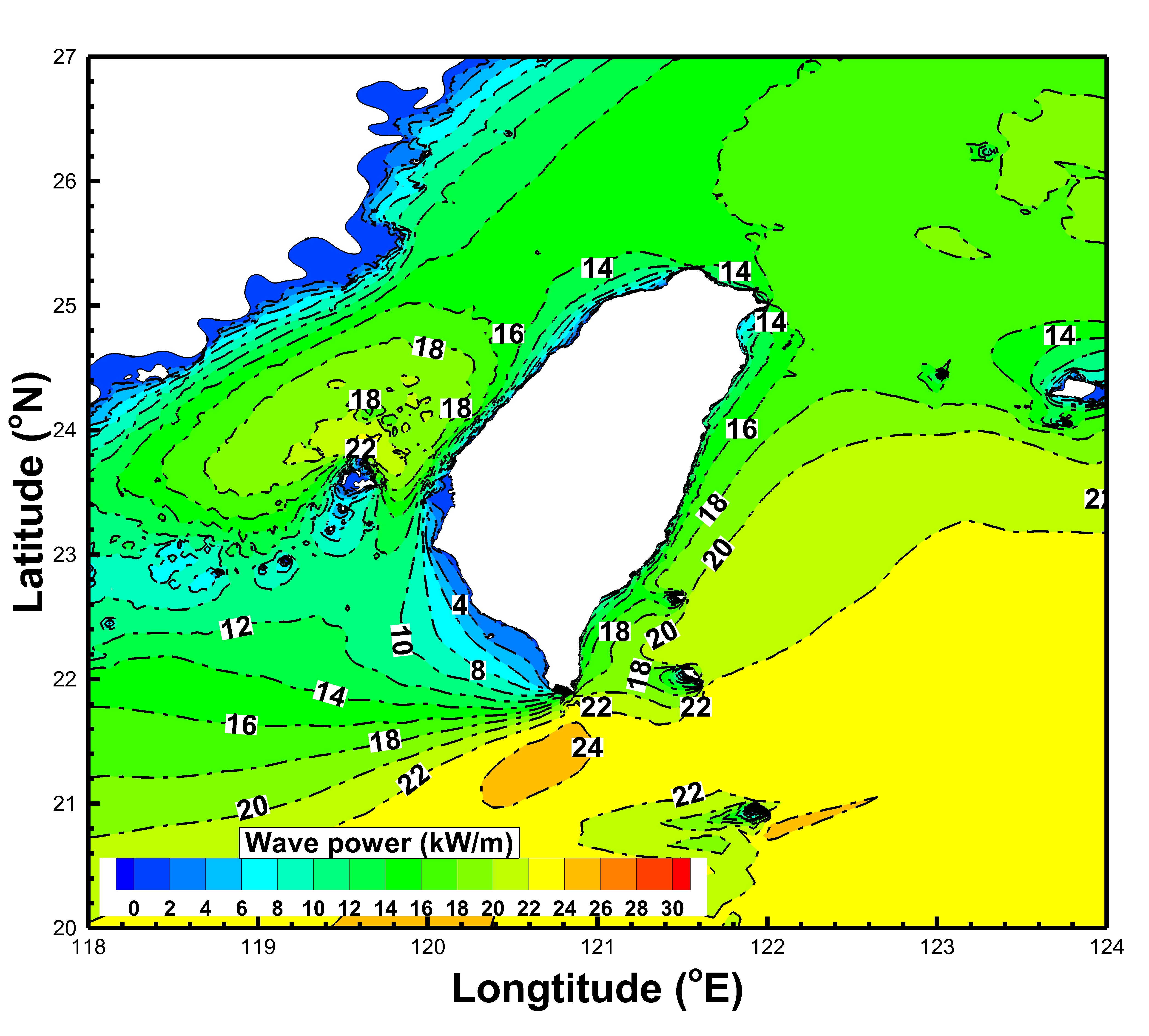
3.2. Spatial Distribution of the Annual Average Wave Power

SCHISM-WWM-III outputted the hourly SWH and peak wave period in each grid, and then the WPD was computed by means of Equation (11). The spatial distributions of the offshore annual average WPD (in kW/m) in the Taiwanese waters from 1991 to 2000 and from 2001 to 2010 are shown in Figure 7 and Figure 8, respectively. The most energetic sea areas are located along the southern and southeastern waters of Taiwan, with the annual mean WPD reaching 28–30 kW/m in 1991 (Figure 7). The sea area in the Central Taiwan Strait (i.e., the Penghu Islands) is another sea area rich in wave power. The highest annual mean WPD was 26 kW/m in 2000 (Figure 7). The annual average WPD was more abundant in 1991, 1992, 1994, 1996, 1999, 2000, 2004, 2005, 2007 and 2008, while 2002 had the smallest annual mean WPD (Figure 8). The offshore WPD in each grid was averaged over 20 years from 1991 to 2010, and the corresponding spatial distribution is presented in Figure 9. The offshore areas lying between Green Island and Orchid Island (Figure 3b), southeast of Orchid Island (Figure 3c), south of the Hengchun Peninsula (Figure 3d), and north of the Penghu Islands (as shown in Figure 3e) were found to be more energetic, with long-term average WPDs of 20, 22, 24 and 22 kW/m, respectively.

3.3. Spatial Distribution of the Monthly Average Wave Power

Figure 10 displays maps of the spatial distribution of the mean WPD for each month in the waters surrounding Taiwan. The gridded WPD was also averaged over the 20 years from 1991 to 2010 for each month. October was characterized by the most abundant monthly mean WPD—approximately 35–40 kW/m for the sea areas surrounding Green Island and Orchid Island and southeast of Orchid Island. South of the Hengchun Peninsula and north of the Penghu Islands, the highest monthly mean WPD of 40 kW/m occurred in November. A weaker monthly average WPD in the range of 8 kW/m–12 kW/m was detected from April to June along the southern and southeastern offshore areas (Figure 10), and the least energetic months were May, June, July, and August for the Central Taiwan Strait, with a monthly mean WPD of only 2 kW/m–7 kW/m (Figure 10).

3.4. Annual and Monthly Average Incidence for the Exploitable Wave Power

Due to the purchase and deployment costs of wave energy converters, the sea area is worthy of exploitation only when the WPD exceeds 2 kW/m [14,60,61,62]. To guarantee this requirement, only WPDs equal to or greater than 4 kW/m were included in the calculation of the incidence of exploitable wave power. The spatial distribution of the incidence (in percentages) of the WPD exceeding 4 kW/m in the offshore waters of Taiwan averaged over 1991 to 2010 is depicted in Figure 11. The highest incidences appear to be 70%–90% southeast of Taiwan, while the lowest incidence is only 30% in the nearshore southwestern waters off Taiwan. The sea area around the northern Penghu Islands exhibited a 50% annual mean WPD incidence. Similarly, Figure 12 describes the monthly average incidence for the WPD exceeding 4 kW/m in the waters surrounding Taiwan from 1991 to 2010. The monthly mean incidences along the eastern waters of Taiwan are approximately 100% in November, and they are always greater than 50% along the southeastern offshore areas every month. In July, the minimum monthly average incidence of 10% occurred in the Central Taiwan Strait; however, the monthly average incidences reached 80% in October, November, December, and January in the same sea area.

3.5. Variability of Wave Power

Sea areas with a steady and constant WPD are more appropriate for the deployment of wave energy converters than WPD areas that are more energetic but unstable [63]. To evaluate the temporal variability of the WPD in the offshore waters of Taiwan, the MVI and COV were calculated via Equations (13) and (14), respectively. The offshore areas displayed a relatively low MVI, and the COV presented weaker temporal variability; therefore, these offshore areas are considered to be potential zones for installing wave energy converters [64,65]. The spatial distribution of the MVI for the WPD in the offshore waters of Taiwan averaged over 1991 to 2010 is depicted in Figure 13. The MVI ranges between 1.8 and 2.7; the maximum MVI is located near the northern Penghu Islands (in the Central Taiwan Strait), and the minimum MVI appears in the northwestern waters of Taiwan, while an MVI of 2.4 is found along the southern and southeastern Taiwanese waters. Figure 14 exhibits the spatial distribution of the COV for the WPD in the waters surrounding Taiwan averaged over 1991 to 2010. The highest and lowest COVs are 2.5 and 1.5 in the southwestern nearshore and northwestern offshore waters of Taiwan, respectively. Moreover, a COV of 2.0 is discovered in the Central Taiwan Strait and the southern and southwestern offshore areas of Taiwan.

3.6. Determination of Optimal Wave Energy Hotspots

The hotspots for deploying wave energy converters were determined according to the assessments of the annual mean WPD, incidence of the exploitable WPD, and MVI and COV of the WPD, as well as the distance between the coast and wave energy conversion devices. Four offshore regions located between Green Island and Orchid Island (hereafter OH_1, as shown in Figure 3b), southeast of Orchid Island (hereafter OH_2, as shown in Figure 3c), south of the Hengchun Peninsula (hereafter OH_3, as shown in Figure 3d), and north of the Penghu Islands (hereafter OH_4, as shown in Figure 3e) were considered the optimal hotspots for the deployment of wave energy converters. These areas are consistent with the spatial distributions of relatively high WPD and incidence but lower MVI and COV. The monthly mean, maximum and minimum WPDs averaged over 1991 to 2010 for OH_1, OH_2, OH_3 and OH_4 are illustrated in Figure 15. The monthly maximum WPD exceeded 90 kW/m for OH_1, OH_2 and OH_3 in October and November and was approximately 100 kW/m for OH_4 in November. The monthly average WPD reached 30 kW/m–50 kW/m for OH_1, OH_2, OH_3 and OH_4 in October to December, while the monthly minimum WPD approached only 20 kW/m for the four optimal hotspots in December. Furthermore, the long-term directional distributions of the WPD were analyzed because the wave direction is an important parameter for the placement of a wave energy converter [35,66]. Figure 16 presents rose diagrams of the WPD for each of the four optimal wave energy hotspots averaged over 1991 to 2010. The dominant WPD directions lie between the east and northeast for OH_1, OH_2 and OH_3; however, the northeast is the prevailing WPD direction within OH_4. The characteristics of the selected optimal wave energy hotspots, such as the coordinates and water depths, are listed in

Table 4. Characteristics of the selected optimal wave energy hotspots.

Buoy	Optimum Hotspots for the Deployment of Wave Energy Converters
	OH_1	OH_2	OH_3	OH_4
Lat. (°), Lon. (°)	(121.48, 22.34)	(121.65, 21.89)	(120.77, 21.49)	(119.64, 23.94)
Water depth (m)	-1268	-1360	-427	-71
WPm (kW/m)	21.03	22.62	24.91	22.33
WEt (MWh/m)	184.22	198.15	218.21	195.61
WEe (MWh/m)	158.06	182.89	196.39	101.33

“-” is the symbol for water depth below mean sea level; WP_m is the annual mean wave power; annual total wave energy outputs; WE_t is the annual total wave energy outputs; WE_e is the exploitable annual wave energy output.

.

4. Discussion

The wave power is weak from March to June for OH_1, OH_2 and OH_3 and from April to August for OH_4, while the wave power is stronger from October to February for all four optimal hotspots. Additionally, the prevailing WPD directions for all optimal hotspots are nearly northeast. This phenomenon might be attributable to the prevalence of the northeast monsoon during late September to early May in Taiwan [67,68]. Alternatively, the long-term statistical data (from 1991 to 2019) issued by the CWB reveal that July, August, and September constitute the typhoon season in Taiwan; however, higher WPDs occur outside of the typhoon season. Although large waves are indeed induced by typhoons, the wave power in the offshore waters of Taiwan is driven mainly by the strong northeast monsoon. Moreover, the deeper water bathymetry also contributes to an increase in the WPD at these hotspots.

By applying Equation (12) with a given Δt_i equal to 8760 h, the annual total wave energy outputs (WE_t) for the four optimal hotspots were calculated, and the results are summarized in Table 4. WE_t values of 184.22, 198.15, 218.21, and 195.61 MWh/m were estimated for OH_1, OH_2, OH_3, and OH_4, respectively, which are more than double the results of a previous study in the same offshore waters [35,57]. The reason for such underestimated values is that the previous studies used wind field data with a temporal resolution of 6 h and a spatial resolution of 0.125° from the ERA-Interim dataset, and the ERA-Interim global reanalysis is inferior to a regional high-resolution dynamical scaling atmospheric model in the performance of wind speeds. This is particularly true under severe weather conditions, e.g., strong monsoons or typhoons. In other words, the wave energy resources and the optimal hotspots for wave energy evaluated in the present study are more reliable than the results from previous studies [35,57]. The exploitable annual wave energy outputs (WE_e) for the hotspots were also assessed, where only Δt_i was replaced by the total hours corresponding to the WPD equal to or greater than 4 kW/m, i.e., 8760 h multiplied by an annual mean incidence. The estimations of WE_e for OH_1, OH_2, OH_3, and OH_4 are 158.06, 182.89, 196.39, and 101.33 MWh/m, respectively (as listed in Table 4).

5. Summary and Conclusions

A three-layer nested Weather Research and Forecast (WRF) model with 45 km, 15 km and 5 km spatial resolutions for Domain 1, Domain 2, and Domain 3, respectively, was implemented over Taiwan and its offshore islands. The high-resolution WRF model was used to downscale the Climate Forecast System Reanalysis (CFSR) product dynamically. The hourly winds 10 m above sea level derived from the WRF model (CFSR_5km) and extracted from CFSR during the period of 2010 served as the meteorological boundary conditions for SCHISM-WWM-III, a fully coupled wave-circulation model. The validation results revealed that the hindcasting performance of SCHISM-WWM-III for the wave parameters, such as significant wave height (SWH), peak wave period and wave direction, by employing the winds from CFSR_5km was superior to those adopting the CFSR wind field. Therefore, the long-term sea states covering the period from 1991 to 2010 were hindcasted through the combination of CFSR_5km winds with SCHISM-WWM-III for assessing the offshore wave energy resources in Taiwan. The spatial distribution of the annual wave power density (WPD) averaged over twenty years shows that the offshore areas between Green Island and Orchid Island (OH_1), southeast of Orchid Island (OH_2), south of the Hengchun Peninsula (OH_3), and north of the Penghu Islands (OH_4) are more energetic than other regions, with long-term annual average WPDs of 20, 22, 24 and 22 kW/m, respectively. An analysis of the monthly mean WPDs over twenty years showed that the greatest WPD is observed from October to January, which means that the wave power is driven mainly by the northeast monsoon in the surrounding waters of Taiwan, even though typhoons can induce extreme waves. The annual average WPD, incidence of the hourly WPD greater than or equal to 4 kW/m, monthly variability index (MVI) and coefficient of variation (COV) for the WPD indicate that sea areas OH_1, OH_2, OH_3 and OH_4 can be considered appropriate sites for deploying wave energy converters. The exploitable long-term annual average total wave energy outputs are estimated to be 158.06, 182.89, 196.39, and 101.33 MWh/m for hotspots OH_1, OH_2, OH_3, and OH_4, respectively. Additionally, northeast is the primary wave direction for each of the four hotspots. The approach proposed by the present study could be applied elsewhere in the world, especially for a regional-scale study of wave power resources. As for evaluating the global wave energy resources, the reanalysis product is sufficient to reflect the distribution of wave energy worldwide.

References

1. Doyle, S.; Aggidis, G.A. Development of multi-oscillating water columns as wave energy converters. Renew. Sustain. Energy Rev. 2019, 107, 75–86. [Google Scholar] [CrossRef] [Green Version]
2. Cruz, J. Ocean Wave Energy—Current Status and Future Prospects; Springer AG: Cham, Switzerland, 2008. [Google Scholar]
3. Aderinto, T.; Li, H. Ocean Wave Energy Converters: Status and Challenges. Energies 2018, 11, 1250. [Google Scholar] [CrossRef] [Green Version]
4. Gunn, K.; Stock-Williams, C. Quantifying the global wave power resource. Renew. Energy 2012, 44, 296–304. [Google Scholar] [CrossRef]
5. Pérez-Collazo, C.; Greaves, D.; Iglesias, G. A review of combined wave and offshore wind energy. Renew. Sustain. Energy Rev. 2015, 42, 141–153. [Google Scholar] [CrossRef] [Green Version]
6. Neill, S.P.; Vogler, A.; Goward-Brown, A.J.; Baston, S.; Lewis, M.J.; Gillibrand, P.A.; Waldman, S.; Woolf, D.K. The wave and tidal resource of Scotland. Renew. Energy 2017, 114, 3–17. [Google Scholar]
7. Fairley, I.; Lewis, M.; Robertson, B.; Hermer, M.; Masters, I.; Horrillo-Caraballo, J.; Karunarathna, H.; Reeve, D.E. A classification system for global wave energy resources based on multivariate clustering. Appl. Energy 2020, 262, 114515. [Google Scholar] [CrossRef]
8. Arinaga, R.A.; Cheung, K.F. Atlas of global wave energy from 10 years of reanalysis and hindcast data. Renew. Energy 2012, 39, 49–64. [Google Scholar] [CrossRef]
9. Reguero, B.G.; Losada, I.J.; Mendez, F.J. A global wave power resource and its seasonal, interannual and long-term variability. Appl. Energy 2015, 148, 366–380. [Google Scholar] [CrossRef]
10. Zhou, G.; Huang, J.; Zhang, G. Elevation of the wave energy conditions along the coastal waters of Beibu Gulf, China. Energy 2015, 85, 449–457. [Google Scholar] [CrossRef]
11. Bento, R.A.; Martinho, P.; Soares, C.G. Numerical modelling of the wave energy in Galway Bay. Renew. Energy 2015, 78, 457–466. [Google Scholar] [CrossRef]
12. Mirzaei, A.; Tangang, F.; Juneng, L. Wave energy potential assessment in the central and southern regions of the South China Sea. Renew. Energy 2015, 80, 454–470. [Google Scholar]
13. Akpmar, A.; Bingolbali, B.; Van Vledder, G.P. Long-term analysis of wave power potential in the Black Sea, Based on 31-year SWAN simulations. Ocean. Eng. 2017, 13, 482–497. [Google Scholar] [CrossRef]
14. Lin, Y.; Dong, S.; Wang, Z.; Guedes Soares, G. Wave energy assessment in the China adjacent seas on the basis of a 20-year SWAN simulation with unstructured grids. Renew. Energy 2019, 136, 275–295. [Google Scholar] [CrossRef]
15. Yang, Z.; García-Medina, G.; Wu, W.-C.; Wang, T. Characteristics and variability of the nearshore wave resource on the U.S. West Coast. Energy 2020, 203, 117818. [Google Scholar] [CrossRef]
16. Gonçalves, M.; Martinho, P.; Soares, C.G. Assessment of wave energy in the Canary Islands. Renew. Energy 2013, 68, 774–784. [Google Scholar] [CrossRef]
17. Inquiry System for Energy Statistical Data, Taiwan. Available online: https://www.moeaboe.gov.tw/wesnq/Views/B01/wFrmB0102.aspx (accessed on 20 January 2021).
18. Saha, S.; Moorthi, S.; Pan, H.-L.; Wu, X.; Wang, J.; Nadiga, S.; Tripp, P.; Kistler, R.; Woollen, J.; Behringer, D.; et al. The NCEP Climate Forecast System Reanalysis. Bull. Amer. Meteorol. Soc. 2010, 91, 1015–1057. [Google Scholar] [CrossRef]
19. Skamarock, W.C.; Klemp, J.B.; Dudhia, J.; Gill, D.O.; Barker, D.M.; Duda, M.G.; Huang, X.Y.; Wang, W.; Powers, J.G. A Description of the Advanced Research WRF Version 3; NCAR Technical Note; NCAR/TN-475 + STR; Mesoscale and Microscale Meteorology Division, National Center for Atmospheric Research: Boulder, CO, USA, 2008. [Google Scholar]
20. Routray, A.; Mohanty, U.; Niyogi, D.; Rizvi, S.; Osuri, K.K. Simulation of heavy rainfall events over Indian monsoon region using WRF-3DVAR data assimilation system. Meteorol. Atmos. Phys. 2010, 106, 107–125. [Google Scholar] [CrossRef]
21. Mohanty, U.; Routray, A.; Osuri, K.K.; Prasad, S.K. A study on simulation of heavy rainfall events over Indian region with ARW-3DVAR modeling system. Pure Appl. Geophys. 2012, 169, 381–399. [Google Scholar] [CrossRef]
22. Routray, A.; Mohanty, U.; Osuri, K.K.; Kar, S.; Niyogi, D. Impact of satellite radiance data on simulations of Bay of Bengal tropical cyclones using the WRF-3DVAR modeling system. IEEE Trans. Geosci. Remote Sens. 2016, 54, 2285–2303. [Google Scholar] [CrossRef]
23. Osuri, K.K.; Nadimpalli, R.; Mohanty, U.C.; Niyogi, D. Prediction of rapid intensification of tropical cyclone Phailin over the Bay of Bengal using the HWRF modelling system. Q. J. R. Meteorol. Soc. 2017, 143, 678–690. [Google Scholar] [CrossRef]
24. Madala, S.; Satyanarayana, A.; Rao, T.N. Performance evaluation of PBL and cumulus parameterization schemes of WRF ARW model in simulating severe thunderstorm events over Gadanki MST radar facility–case study. Atmos. Res. 2014, 139, 1–17. [Google Scholar] [CrossRef]
25. Osuri, K.; Nadimpalli, R.; Mohanty, U.; Chen, F.; Rajeevan, M.; Niyogi, D. Improved prediction of severe thunderstorms over the Indian Monsoon region using high-resolution soil moisture and temperature initialization. Sci. Rep. 2017, 7, 41377. [Google Scholar] [CrossRef] [PubMed] [Green Version]
26. Powers, J.G.; Klemp, J.B.; Skamarock, W.C.; Davis, C.A.; Dudhia, J.; Gill, D.O.; Coen, J.L.; Gochis, D.J. The Weather Research and Forecasting Model: Overview, system efforts, and future directions. Bull. Am. Meteorol. Soc. 2017, 98, 1717–1737. [Google Scholar] [CrossRef]
27. Zhang, Y.J.; Ye, F.; Stanev, E.V.; Grashorn, S. Seamless cross-scale modelling with SCHISM. Ocean. Model. 2016, 102, 64–81. [Google Scholar] [CrossRef] [Green Version]
28. Zhang, Y.J.; Baptista, A.M. SELFE: A semi-implicit Eulerian-Lagrangian finite-element model for cross-scale ocean circulation. Ocean. Model. 2008, 21, 71–96. [Google Scholar] [CrossRef]
29. Shchepetkin, A.F.; McWilliams, J.C. The regional oceanic modeling system (ROMS): A split-explicit, free-surface, topography-following-coordinate, oceanic model. Ocean. Model. 2005, 9, 347–404. [Google Scholar] [CrossRef]
30. Chen, W.-B.; Liu, W.-C. Investigating the fate and transport of fecal coliform contamination in a tidal estuarine system using a three-dimensional model. Marine Pollut. Bull. 2017, 116, 365–384. [Google Scholar] [CrossRef]
31. Chen, W.-B.; Liu, W.-C. Modeling flood inundation Induced by river flow and storm surges over a river basin. Water 2014, 6, 3182–3199. [Google Scholar] [CrossRef] [Green Version]
32. Chen, W.-B.; Liu, W.-C. Assessment of storm surge inundation and potential hazard maps for the southern coast of Taiwan. Nat. Hazards 2016, 82, 591–616. [Google Scholar] [CrossRef]
33. Chen, Y.-M.; Liu, C.-H.; Shih, H.-J.; Chang, C.-H.; Chen, W.-B.; Yu, Y.-C.; Su, W.-R.; Lin, L.-Y. An Operational Forecasting System for Flash Floods in Mountainous Areas in Taiwan. Water 2019, 11, 2100. [Google Scholar] [CrossRef] [Green Version]
34. Chen, W.-B.; Chen, H.; Lin, L.-Y.; Yu, Y.-C. Tidal Current Power Resource and Influence of Sea-Level Rise in the Coastal Waters of Kinmen Island, Taiwan. Energies 2017, 10, 652. [Google Scholar] [CrossRef] [Green Version]
35. Shih, H.-J.; Chang, C.-H.; Chen, W.-B.; Lin, L.-Y. Identifying the Optimal Offshore Areas for Wave Energy Converter Deployments in Taiwanese Waters Based on 12-Year Model Hindcasts. Energies 2018, 11, 499. [Google Scholar] [CrossRef] [Green Version]
36. Shih, H.-J.; Chen, H.; Liang, T.-Y.; Fu, H.-S.; Chang, C.-H.; Chen, W.-B.; Su, W.-R.; Lin, L.-Y. Generating potential risk maps for typhoon-induced waves along the coast of Taiwan. Ocean. Eng. 2018, 163, 1–14. [Google Scholar] [CrossRef]
37. Chen, W.-B.; Chen, H.; Hsiao, S.-C.; Chang, C.-H.; Lin, L.-Y. Wind forcing effect on hindcasting of typhoon-driven extreme waves. Ocean. Eng. 2019, 188, 106260. [Google Scholar] [CrossRef]
38. Hsiao, S.-C.; Chen, H.; Chen, W.-B.; Chang, C.-H.; Lin, L.-Y. Quantifying the contribution of nonlinear interactions to storm tide simulations during a super typhoon event. Ocean. Eng. 2019, 194, 106661. [Google Scholar] [CrossRef]
39. Komen, G.J.; Cavaleri, L.; Donelan, M.; Hasselmann, K.; Hasselmann, S.; Janssen, P.A.E.M. Dynamics and Modelling of Ocean Waves; Cambridge University Press: Cambridge, UK, 1994. [Google Scholar]
40. Hsu, T.W.; Ou, S.-H.; Liau, J.-M. Hindcasting nearshore wind waves using a FEM code for SWAN. Coast. Eng. 2005, 52, 177–195. [Google Scholar] [CrossRef]
41. Roland, A. Development of WWM II: Spectral Wave Modeling on Unstructured Meshes. Ph.D. Thesis, Technology University Darmstadt, Darmstadt, Germany, 2009. [Google Scholar]
42. Yanenko, N.N. The Method of Fractional Steps; Springer: Berlin/Hamburg, Germany, 1971. [Google Scholar]
43. Leonard, B.P. The ultimate conservative difference scheme applied to unsteady one-dimensional advection. Comput. Method. Appl. Mech. 1991, 88, 17–74. [Google Scholar] [CrossRef]
44. Hasselmann, K.; Barnett, T.P.; Bouws, E.; Carlson, H.; Cartwright, D.E.; Enke, K.; Ewing, J.A.; Gienapp, H.; Hasselmann, D.E.; Kruseman, P.; et al. Measurements of Wind-Wave Growth and Swell Decay during the Joint North. Sea Wave Project (JONSWAP); Deutsches Hydrographisches Institut: Berlin/Hamburg, Germany, 1973. [Google Scholar]
45. Roland, A.; Zhang, Y.J.; Wang, H.V.; Meng, Y.; Teng, Y.-C.; Maderich, V.; Brovchenko, I.; Dutour-Sikiric, M.; Zanke, U. A fully coupled 3D wave-current interaction model on unstructured grids. J. Geophys. Res. 2012, 117, C00J33. [Google Scholar] [CrossRef] [Green Version]
46. Hsiao, S.-C.; Chen, H.; Wu, H.-L.; Chen, W.-B.; Chang, C.-H.; Guo, W.-D.; Chen, Y.-M.; Lin, L.-Y. Numerical Simulation of Large Wave Heights from Super Typhoon Nepartak (2016) in the Eastern Waters of Taiwan. J. Mar. Sci. Eng. 2020, 8, 217. [Google Scholar] [CrossRef] [Green Version]
47. Chen, W.-B.; Lin, L.-Y.; Jang, J.-H.; Chang, C.-H. Simulation of Typhoon-Induced Storm Tides and Wind Waves for the Northeastern Coast of Taiwan Using a Tide–Surge–Wave Coupled Model. Water 2017, 9, 549. [Google Scholar] [CrossRef]
48. Hsiao, S.-C.; Wu, H.-L.; Chen, W.-B.; Chang, C.-H.; Lin, L.-Y. On the Sensitivity of Typhoon Wave Simulations to Tidal Elevation and Current. J. Mar. Sci. Eng. 2020, 8, 731. [Google Scholar] [CrossRef]
49. Zhang, H.; Sheng, J. Estimation of extreme sea levels over the eastern continental shelf of North America. J. Geophys. Res. Oceans 2013, 118, 6253–6273. [Google Scholar] [CrossRef]
50. Muis, S.; Verlaan, M.; Winsemius, H.C.; Aerts, J.C.J.H.; Ward, P.J. A global reanalysis of storm surges and extreme sea levels. Nat. Commun. 2017, 7, 11969. [Google Scholar] [CrossRef] [PubMed] [Green Version]
51. Marsooli, R.; Lin, N. Numerical Modeling of Historical Storm Tides and Waves and Their Interactions Along the U.S. East and Gulf Coasts. J. Geophys. Res. Oceans 2018, 123, 3844–3874. [Google Scholar] [CrossRef] [Green Version]
52. Amaechi, C.V.; Wang, F.; Hou, X.; Ye, J. Strength of submarine hoses in Chinese-lantern configuration from hydrodynamic loads on CALM buoy. Ocean. Eng. 2019, 171, 429–442. [Google Scholar] [CrossRef] [Green Version]
53. Zu, T.; Gana, J.; Erofeevac, S.Y. Numerical study of the tide and tidal dynamics in the South China Sea. Deep Sea Res. Part. I 2008, 55, 137–154. [Google Scholar] [CrossRef]
54. Boronowski, S.; Wild, P.; Rowe, A.; G. Cornelis van Kooten, C.G. Integration of wave power in Haida Gwaii. Renew. Energy 2010, 35, 2415–2421. [Google Scholar] [CrossRef]
55. Sierra, J.P.; Moss, A.; Gonzale-Marco, D. Wave energy resource assessment in Menorca (Spain). Renew. Energy 2014, 71, 51–60. [Google Scholar] [CrossRef]
56. Sierra, J.P.; Casas-Prat, M.; Campins, E. Impact of climate change on wave energy resource: The case of Menorca (Spain). Renew. Energy 2017, 101, 275–285. [Google Scholar] [CrossRef]
57. Su, W.-R.; Chen, H.; Chen, W.-B.; Chang, C.-H.; Lin, L.-Y.; Jang, J.-H.; Yu, Y.-C. Numerical investigation of wave energy resources and hotspots in the surrounding waters of Taiwan. Renew. Energy 2018, 118, 814–824. [Google Scholar] [CrossRef]
58. Gonçalves, M.; Martinho, P.; Guedes Soares, C. Wave energy assessment based on a 33-year hindcast for the Canary Islands. Renew. Energy 2020, 152, 259–269. [Google Scholar] [CrossRef]
59. Cornett, A. A global wave energy resource assessment. In Proceedings of the 18th International Offshore and Polar Engineering Conference, Vancouver, BC, Canada, 6–11 July 2008. [Google Scholar]
60. Wan, Y.; Fan, C.; Zhang, J.; Meng, J.; Dai, Y.; Li, L.; Sun, W.; Zhou, P.; Wang, J.; Zhang, Z. Wave Energy Resource Assessment off the Coast of China around the Zhoushan Islands. Energies 2017, 10, 1320. [Google Scholar] [CrossRef] [Green Version]
61. Zheng, C.W.; Pan, J.; Li, J.X. Assessing the China Sea wind energy and wave energy resources from 1988 to 2009. Ocean. Eng. 2013, 65, 39–48. [Google Scholar]
62. Kamranzad, B.; Etemad-Shahidi, A.; Chegini, V. Developing an optimum hotspot identifier for wave energy extracting in the northern Persian Gulf. Renew. Energy 2017, 114, 59–71. [Google Scholar] [CrossRef]
63. Lopez, I.; Andreu, J.; Ceballos, S.; Martínez De Alegría, I.; Kortabarria, I. Review of wave energy technologies and the necessary power-equipment. Renew. Sustain. Energy Rev. 2013, 27, 413–434. [Google Scholar] [CrossRef]
64. Lavidas, G.; Venugopal, V. A 35-year high-resolution wave atlas for nearshore energy production and economics at the Aegean Sea. Renew. Energy 2017, 103, 401–417. [Google Scholar] [CrossRef] [Green Version]
65. Amarouche, K.; Akpınar, A.; El Islam Bachari, N.; Houma, F. Wave energy resource assessment along the Algerian coast based on 39-year wave hindcast. Renew. Energy 2020, 153, 840–860. [Google Scholar] [CrossRef]
66. Atan, R.; Goggins, J.; Nash, S. A Detailed Assessment of the Wave Energy Resource at the Atlantic Marine Energy Test Site. Energies 2016, 9, 967. [Google Scholar] [CrossRef] [Green Version]
67. Tao, S.Y.; Chen, L.X. A review of recent research on East Asian summer monsoon in China. In Monsoon Meteorology; Chang, C.P., Krishnamurti, T.N., Eds.; Oxford University Press: New York, NY, USA, 1987. [Google Scholar]
68. Boyle, J.S.; Chen, G.T.J. Synoptic aspects of the wintertime East Asian monsoon. In Monsoon Meteorology; Chang, C.P., Krishnamurti, T.N., Eds.; Oxford University Press: New York, NY, USA, 1987. [Google Scholar]
Figure 1. Extents of the Weather Research and Forecasting (WRF) model with grid spacings of approximately 45 km for Domain 1 (D01), approximately 15 km for Domain 2 (D02) and approximately 5 km for Domain 3 (D03).
Energies 14 00653 g001
Figure 2. (a) Unstructured grid mesh for the whole computational domain, (b) magnified view of the high-resolution unstructured grid mesh for Green Island and Orchid Island, and (c) magnified view of the high-resolution unstructured grid mesh for the Penghu Islands.
Energies 14 00653 g002
Figure 3. (a) Bathymetry for the whole computational domain and (b) magnified views of the bathymetry for offshore hotspot OH_1, (c) OH_2, (d) OH_3 and (e) OH_4.
Energies 14 00653 g003
Figure 4. Scatter plots of the hindcasted versus measured significant wave heights (SWHs) for the (a,e) Longdong, (b,f) Hualien, (c,g) Hsinchu and (d,h) Xiaoliuqiu buoys using the (ad) Climate Forecast System Reanalysis (CFSR) and (eh) CFSR_5km winds.
Energies 14 00653 g004
Figure 5. Scatter plots of the hindcasted versus measured peak wave periods for the (a,e) Longdong, (b,f) Hualien, (c,g) Hsinchu and (d,h) Xiaoliuqiu buoys using the (ad) CFSR and (eh) CFSR_5km winds.
Energies 14 00653 g005
Figure 6. Scatter plots of the hindcasted versus measured wave directions for the (a,e) Longdong, (b,f) Hualien, (c,g) Hsinchu and (d,h) Xiaoliuqiu buoys using the (ad) CFSR and (eh) CFSR_5km winds.
Energies 14 00653 g006
Figure 7. Spatial distributions of the annual average wave power in the offshore waters of Taiwan from 1991 to 2000.
Energies 14 00653 g007
Figure 8. Spatial distributions of the annual average wave power in the offshore waters of Taiwan from 2001 to 2010.
Energies 14 00653 g008
Figure 9. Spatial distribution of the wave power in the offshore waters of Taiwan averaged over 1991 to 2010.
Energies 14 00653 g009
Figure 10. Spatial distributions of the monthly average wave power in the offshore waters of Taiwan from 1991 to 2010.
Energies 14 00653 g010aEnergies 14 00653 g010b
Figure 11. Spatial distribution of the incidence of the wave power exceeding 4 kW/m in the offshore waters of Taiwan averaged over 1991 to 2010.
Energies 14 00653 g011
Figure 12. Spatial distributions of the monthly average incidence of the wave power exceeding 4 kW/m in the offshore waters of Taiwan from 1991 to 2010.
Energies 14 00653 g012aEnergies 14 00653 g012b
Figure 13. Spatial distribution of the monthly variability index (MVI) of wave power in the offshore waters of Taiwan averaged over 1991 to 2010.
Energies 14 00653 g013
Figure 14. Spatial distribution of the coefficient of variation (COV) of wave power in the offshore waters of Taiwan averaged over 1991 to 2010.
Energies 14 00653 g014
Figure 15. Monthly mean, maximum and minimum wave powers from 1991 to 2010 for four optimal wave energy hotspots: (a) OH_1, (b) OH_2, (c) OH_3, and (d) OH_4.
Energies 14 00653 g015aEnergies 14 00653 g015b
Figure 16. Directional distributions of the wave power averaged over 1991 to 2010 for four optimal wave energy hotspots: (a) OH_1, (b) OH_2, (c) OH_3 and (d) OH_4.
Energies 14 00653 g016