Research on Model Predictive Control for Automobile Active Tilt Based on Active Suspension

Abstract

To improve the handling stability of automobiles and reduce the odds of rollover, active or semi-active suspension systems are usually used to control the roll of a vehicle. However, these kinds of control systems often take a zero-roll-angle as the control target and have a limited effect on improving the performance of the vehicle when turning. Tilt control, which actively controls the vehicle to tilt inward during a curve, greatly benefits the comprehensive performance of a vehicle when it is cornering. After analyzing the advantages and disadvantages of the tilt control strategies for narrow commuter vehicles by combining the structure and dynamic characteristics of automobiles, a direct tilt control (DTC) strategy was determined to be more suitable for automobiles. A model predictive controller for the DTC strategy was designed based on an active suspension. This allowed the reverse tilt to cause the moment generated by gravity to offset that generated by the centrifugal force, thereby significantly improving the handling stability, ride comfort, vehicle speed, and rollover prevention. The model predictive controller simultaneously tracked the desired tilt angle and yaw rate, achieving path tracking while improving the anti-rollover capability of the vehicle. Simulations of step-steering input and double-lane change maneuvers were performed. The results showed that, compared with traditional zero-roll-angle control, the proposed tilt control greatly reduced the occupant’s perceived lateral acceleration and the lateral load transfer ratio when the vehicle turned and exhibited a good path-tracking performance.

1. Introduction

Vehicle roll dynamics affects the handling stability and ride comfort. When cornering at high speeds, a vehicle is prone to excessive rolling, which can cause the vehicle to become unstable or to rollover. The traditional passive suspension has difficulty meeting the performance requirements of vehicles with suspension systems. Suspension control technologies, such as active and semi-active suspensions, active lateral stabilizer bars, and hydraulic interconnected suspensions, are often used to prevent automobile rolling [1,2,3,4]. However, the current roll control methods usually aim at passively reducing the roll angle and have limited effects on improving the vehicle’s performance during cornering.

Drawing on the tilting technology used on rail trains [5], if the automobile body is tilted in the turning direction, this reverse tilt can cause the moment generated by gravity to reduce or even offset that generated by the centrifugal force. This novel technology can significantly improve the handling stability and the ride comfort. After years of research, the active tilting technology has been widely used in high-speed rail trains [5,6]. A previous study [7] indicated that on a current track line, only tilting the train at a small angle (1–2°) can allow the vehicle to negotiate the curve at a sufficiently high speed. Therefore, tilting at a small angle can also greatly improve the vehicle performance. Because rail trains and automobiles are very different in structure and driving conditions, there are very few things that can be learned for the study of tilt control.

Narrow commuter vehicles (NCVs) which attracted the interest of researchers in the past decades rely heavily on tilt control due to their high centers of gravity, and much research has been conducted on tilt control of these vehicles [8,9]. Several researchers developed test prototypes. Most control strategies for NCVs can be classified as steering tilt control (STC) and direct tilt control (DTC) [10]. The DTC strategy is controlled by a special actuator installed under the vehicle body, while the STC strategy uses active counter-steering to control the vehicle steering to achieve active tilt. Rajamani and his group have studied the active tilt control of NCVs [8,11]. Nguyen et al. presented a DTC method to improve the lateral stability and the driving comfort of narrow tilting vehicles. An H₂ control design based on a linear matrix inequality based optimization was built. The resulting robust DTC controller was evaluated with realistic driving scenarios [12].

Due to the structural characteristics of NCVs, the DTC strategy is suitable for low speeds, and the STC strategy is suitable for high speeds [13]. Some work has thus focused on combining these two control strategies to achieve stability at all vehicle speeds. Rajamani’s group presented a combination control system with two different types of control schemes. The performances of the proposed integrated systems were evaluated by carrying out simulations and experimental work [14]. Robertson et al. presented a method for integrating the STC and DTC strategies. The control systems exhibited a 36% reduction in load transfer from the inside wheel to the outside wheel during a ramp-steering maneuver compared with a DTC system [15].

Research on tilt control of automobiles began relatively late compared to the tilt control research of trains and NCVs, but it is currently attracting researchers’ interest. Wang expounded the feasibility of tilt control based on an active suspension system under low-speed steering conditions and designed a vehicle active-tilting robust H-infinity controller while considering ride comfort and handling stability [16]. Simulation results showed that lateral acceleration was reduced and that vertical and pitch motions were effectively restrained. Ling studied SUVs and adopted a slow active suspension system to achieve “body reverse roll control” (i.e., tilt control) [17]. The control strategy was designed based on fuzzy adaptive PID control. Joint MATLAB/Simulink, AMESim, and Carsim simulations were carried out and showed that this type of tilt control effectively improved the stability and safety of the vehicle without lessening the ride comfort. Youn et al. used active suspension to implement active tilt control to control the attitude of the vehicle [18]. An attitude-tracking controller was designed with zero acceleration as the target; simulation results verified the feasibility of the controller. Afterwards, integrated control research of active tilt control and the electronic stability program was carried out [19]. Zhu et al. obtained the optimal roll angle and yaw rate based on road preview information of unmanned vehicles. They designed a model predictive controller through active suspension to intentionally increase the roll angle inward or outward as needed [20]. However, this publication did not explicitly discuss the rolling problem using the concept of vehicle tilt. Rajamani et al. presented a new steer-by-wire algorithm that used transient counter-steering to invert the direction of the roll angle of the vehicle to reduce to odds of rollover. However, this STC strategy could only operate in the stable equilibrium position, in which the tilting angle usually exceeded the effective travel distance of the suspension [21]. To date, no active tilt control technology has been used in actual automobiles. Some automobile companies claim that they have used the active tilt control technology; however, they only used traditional active roll control technology that minimizes the vehicle’s body lean during cornering, such as the active tilt control (ATC) used by some SUVs belonging to brands from the Ford Motor Company [22].

To date, research on automobile tilt control has not been conducted in a systematic way. It is necessary to study control strategy designs, determine the appropriate actuator, and further elaborate the meaning and evaluation method of automobile active tilt. The structural and dynamic characteristics of automobiles are different from those of NCVs, and the speeds are much higher; therefore, the tilt control strategies are also different from those of NCVs. Among the two tilt control strategies for NCV vehicles, the STC strategy must increase the steering angle at low speeds to maintain stability [23]. However, automobiles run stably at low speeds, but at high speeds, because STC systems can only operate in a steady-state equilibrium position in which the desired tilt angle is used, the tilt angle is often too large. Thus, STC systems are not suitable for controlling automobile tilt. DTC systems require the active tilting and steering to be synchronized to reduce actuator torque and improve ride comfort. With the development of sensor technologies, it is easy for automobiles to preview the driver’s steering input through GPS and map information. Meanwhile, once a vehicle is tilted slightly inward, the gravitational force begins to assist the tilt actuator, which lowers the power required [24]. Therefore, the DTC strategy is more suitable for automobiles.

Based on the above analysis and previous research [25], a DTC strategy for automobiles is proposed herein based on an active suspension using model predictive control technology. Based on the automobile structure and performance characteristics, an automobile tilt control model was established, and a tilt control strategy and performance evaluation method were proposed. Considering the performance requirements in the vehicle roll and yaw directions, a model predictive controller was designed to enable the vehicle to track the desired tilting angle while tracking the desired yaw rate in real time. This article focuses on the elaboration of the vehicle tilt control methodology, and, thus, it ignores the influence of signal acquisition and road interference on the controller design [26,27,28]. Simulations were performed under step-steering input and double-lane change maneuvers. Meanwhile, the designed tilt controller was compared with passive suspension and a traditional anti-roll controller that aimed to achieve a zero-roll-angle as the control target. Finally, the advantages of this tilt controller over the traditional zero-roll-angle controller for improving vehicle performance were analyzed.

The remainder of this article is organized as follows: the steer–roll dynamic models of an active suspension vehicle are developed in Section 2; on Section 3, the desired tilt angle for active tilt control is determined, and a model predictive controller with two tracking aims is developed; the simulations are discussed in Section 4; finally, the conclusions are presented in Section 5.

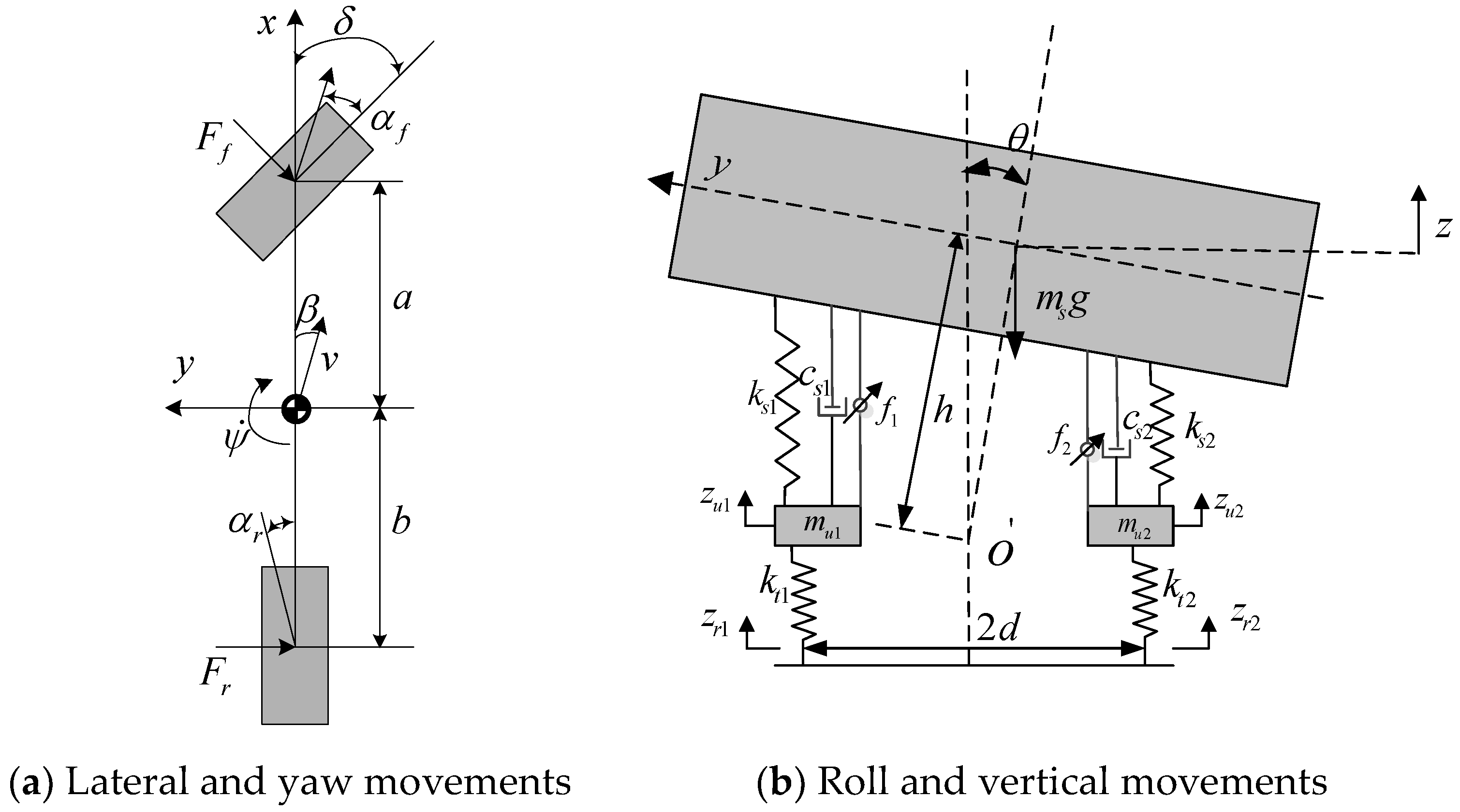
2. Vehicle Steer–Roll Dynamic Model Based on Active Suspension

A six-degree-of-freedom (6-DOF) vehicle steer–roll dynamic model with a two-degree-of-freedom (2-DOF) steering model and a 4-DOF roll model was developed to study the dynamics of vehicle active tilt during cornering. The established vehicle model is shown in Figure 1. Based on D’ Alembert’s principle, the dynamic equations of the vehicle model are as follows:

Vehicle steering dynamics equation:

$$mv(\dot{\beta }+\dot{\psi })+m_{s}h\ddot{\theta }=2F_f+2F_r$$

(1)

$$I_z\ddot{\psi }=2a{F}_f-2b{F}_r$$

(2)

For Equations (1) and (2), to make the analysis of vehicle motion simpler, a four-wheeled vehicle was transformed to an equivalent two-wheeled vehicle [29]. It is assumed that the lateral tire forces $F_f$ and $F_r$ are proportional to the tire slip angle for small angles, and $\left|\beta \right|$ is considered to be very small. Additionally, if the vehicle speed is constant, $v=\sqrt{v_x^2+v_y^2}$ is also constant. Thus, $v_x=v\cos \beta \approx v$, and $v_y=v\sin \beta \approx v\beta$. Then the front and rear tire side-slip angles can be written as shown below:

$${\alpha }_f\approx -(\delta -\frac{v_y+a\dot{\psi }}{v})\approx \beta +\frac{a\dot{\psi }}{v}-\delta$$

(3)

$${\alpha }_r\approx \frac{v_y-b\dot{\psi }}{v}\approx \beta -\frac{b\dot{\psi }}{v}$$

(4)

The lateral tire forces can be expressed as follows:

$$F_f=-{\mathrm{c}}_f{\alpha }_f=-{\mathrm{c}}_f(\beta +\frac{a\dot{\psi }}{v}-\delta )$$

(5)

$$F_r=-{\mathrm{c}}_r{\alpha }_r=-{\mathrm{c}}_r(\beta -\frac{b\dot{\psi }}{v})$$

(6)

Dynamics equation of sprung mass vertical motion:

$$m_s\ddot{z}=F_{s1}+F_{s2}+f_1+f_2$$

(7)

Dynamics equation of vehicle roll motion:

$$I_x\ddot{\theta }=(F_{s1}-F_{s2})d-m_{s}v(\dot{\beta }+\dot{\psi })h+m_{s}gh\theta +M_t$$

(8)

Dynamics equation of unsprung mass vertical movement:

$$m_{\mathrm{u}1}{\ddot{z}}_{u1}=-F_{s1}-k_{t1}(z_{u1}-z_{r1})-f_1$$

(9)

$$m_{\mathrm{u}2}{\ddot{z}}_{u2}=-F_{s2}-k_{t2}(z_{u1}-z_{r2})-f_2$$

(10)

The variables used for this vehicle model are defined as follows: $\dot{\psi }$ is the yaw rate; $\theta$ is the roll angle; $\beta$ is the side-slip angle at the vehicle center of gravity (CG); $y$ is the lateral displacement of the vehicle; $z$ is the vertical displacement of the CG of the sprung mass; $z_{u1}$ and $z_{u2}$ are the vertical displacements of the unsprung masses of the left and right suspensions, respectively; $z_{r1}$ and $z_{r2}$ are the road input on the left and right wheels, respectively; m is the total mass of the vehicle, $m_s$ is the sprung mass of the vehicle; $m_{\mathrm{u}1}$ and $m_{\mathrm{u}2}$ are the unsprung masses of the left and right suspensions, respectively; $I_x$ and $I_z$ are the mass moments inertia about the x- and z-axes, respectively; ${\mathrm{c}}_f$ and ${\mathrm{c}}_r$ are the cornering stiffnesses of the front and rear tires, respectively; $k_{t1}$ and $k_{t2}$ are the vertical stiffnesses of the left and right tires, respectively; $h$ is the height of sprung mass from roll center; $a$ and $b$ are the distances from the CG to the front or rear axle, respectively; $d$ is half of the track width; $\delta$ is the front steering angle; v is the longitudinal velocity of the vehicle; $f_1$ and $f_2$ are the controllable damping forces of the left and right suspensions, respectively; $M_t$ is the tilting torque generated by the active suspension actuating struts, which can be written as $M_t=(f_1-f_2)d$; $\delta$ is the steering angle of the front wheel.

The dynamic forces of the left and right suspensions due to vertical acceleration can be written as follows:

$$F_{s1}=-k_{s1}(z_{s1}-z_{u1})-c_{s1}({\dot{z}}_{s1}-{\dot{z}}_{u_1})$$

(11)

$$F_{s2}=-k_{s2}(z_{s2}-z_{u2})-c_{s2}({\dot{z}}_{s2}-{\dot{z}}_{u_2})$$

(12)

In Equations (11) and (12), $k_{s1}$ and $k_{s2}$ are the spring stiffness coefficients of the left and right suspensions, respectively; $c_{s1}$ and $c_{s2}$ are the constant damping coefficients of the left and right suspensions, respectively; $z_{s1}$ and $z_{s2}$ are the vertical displacements of the sprung mass on the left and right, respectively, which can be expressed as follows:

$$z_{s1}=z+d\theta ,\hspace{1em}{z}_{s2}=z-d\theta$$

(13)

$${\dot{z}}_{s1}=\dot{z}+d\dot{\theta },\hspace{1em}{\dot{z}}_{s2}=\dot{z}-d\dot{\theta }$$

(14)

3. Design of the Model Predictive Controller

3.1. Desired Tilt Angle for Active Tilt Control

When turning, the vehicle body actively tilts inward, causing the gravity moment on the vehicle body to offset the centrifugal force moment on the vehicle body. Therefore, the values of the lateral acceleration experienced by passengers and the lateral load transfer ratio will be reduced greatly or even to zero. The roll moment generated by the centrifugal force is as follows:

$$M_{steer}=m_{s}v(\dot{\beta }+\dot{\psi })h\cos \theta =m_s(\ddot{y}+v\dot{\psi })h\cos \theta$$

(15)

The roll moment generated by gravity is as follows:

$$M_G=m_{s}gh\sin \theta$$

(16)

When the vehicle is at steady state, $\ddot{y}=0$ and $\dot{\psi }={\dot{\psi }}_{des}=\delta \frac{v}{a+b}$, which is the yaw rate of the ideal steering model with two DOFs (in neutral steering). The desired tilt angle for the active tilt can be obtained via $M_{steer}=M_G$:

$${\theta }_{des}=\arctan \left(\frac{\mathrm{v}{\dot{\psi }}_{des}}{g}\right)$$

(17)

The occupant’s perceived lateral acceleration is mainly composed of three parts, namely the lateral acceleration $a_y$, the component of gravitational acceleration, and the roll acceleration of the vehicle body, which can be expressed as follows:

$$a_{per}=v(\dot{\beta }+\dot{\psi })\cos \theta +h\ddot{\theta }-g\sin \theta$$

(18)

The lateral load transfer ratio (LTR) is a commonly used indicator for predicting non-tripping rollover of vehicles and can be expressed as follows [30]:

$$LTR=\frac{m_{s}v(\dot{\beta }+\dot{\psi })h+I_x\ddot{\theta }-m_{s}gh\theta }{m_{s}gd}$$

(19)

The block diagram of the active tilt model predictive control system is shown in Figure 2.

3.2. Design of the Controller

The model predictive control algorithm is used to control the active suspension actuator in real time so that the actual tilt angle of the active tilt can track the desired tilt angle. The state space of the vehicle suspension system based on the 6-DOF vehicle steer–roll model is as follows:

$$\{\begin{array}{c}\dot{\xi }=A_c\xi +B_{cu}u+B_{cd}w\hfill \\ \eta =C_c\xi \hfill \end{array}$$

(20)

where the system states are $\xi ={[\beta ,\dot{\psi },\theta ,\dot{\theta },z,\dot{z},z_{u1},{\dot{z}}_{u1},z_{u2},{\dot{z}}_{u2}]}^T$, the control inputs are $u={\left[f_1,f_2\right]}^T$, the system disturbances are $w={[z_{r1},z_{r2},\delta ]}^{{}_T}$, the system outputs are $\eta ={[\dot{\psi },\theta ]}^T$, and the parameters of matrices are as listed in the Appendix A.

The 6-DOF vehicle steer–roll dynamic model established above is a linear continuous system model. Based on model predictive control theory, the continuous system should first be discretized by a matrix exponential transformation. This can be expressed as follows:

$$\{\begin{array}{c}\xi (k+1)=A\xi (k)+B_{u}u(k)+B_{d}w(k)\hfill \\ \eta (k)=C_c\xi (k)\hfill \end{array}$$

(21)

where $A=e^{A_c{T}_s}$,$B_u={\displaystyle {\int }_0^{T_s}{e}^{A_c\tau }{B}_{cu}d}\tau$,$B_d={\displaystyle {\int }_0^{T_s}{e}^{A_c\tau }{B}_{cd}d}\tau$, and $T_s$ is the sampling period.

To prevent the control variable of the model predictive controller from changing too much and to constrain the control increment, the control variable $u(k)$ in Equation (21) is rewritten in terms of the control increment $\Delta u(k)$, yielding the following augmented model:

$$\{\begin{array}{c}\tilde{\xi }(k+1)=\tilde{A}\tilde{\xi }(k)+{\tilde{B}}_u\tilde{u}(k)+{\tilde{B}}_d\tilde{w}(k)\hfill \\ \eta (k)={\tilde{C}}_c\tilde{\xi }(k)\hfill \end{array}$$

(22)

The matrices in this formula are defined as follows:

$$\tilde{\xi }(k)=\left[\begin{array}{c}\xi (k)\\ u(k-1)\end{array}\right],\tilde{w}(k)=\left[\begin{array}{c}w(k)\\ 0_{N_u}\end{array}\right],\tilde{\xi }(k)=\left[\begin{array}{c}\xi (k)\\ u(k-1)\end{array}\right],\tilde{w}(k)=\left[\begin{array}{c}w(k)\\ 0_{N_u}\end{array}\right],$$

$$\tilde{A}=\left[\begin{array}{cc}A& B_u\\ 0_{N_u\times N_{\xi }}& I_{N_u}\end{array}\right],{\tilde{B}}_u=\left[\begin{array}{c}{B}_u\\ I_{N_u}\end{array}\right],$$

$${\tilde{B}}_d=\left[\begin{array}{c}{B}_d\\ 0_{N_u\times N_d}\end{array}\right],{\tilde{C}}_c=\left[\begin{array}{cc}{C}_c& 0_{N_u}\end{array}\right],$$

$$\tilde{u}(k)=\Delta u(k)=u(k)-u(k-1),$$

where $N_{\xi }$ is the number of states, $N_d$ is the number of disturbances, and $N_u$ is the number of control inputs.

If the predicted horizon of the system is $N_p$ and the control horizon is $N_c$, to derive the system’s predictive equations, the following two assumptions are made.

The control variables remain unchanged outside the control horizon:

$$\Delta u(k+i)=0,i=Nc,Nc+1,\cdots ,N_p-1$$

(23)

The disturbances remain unchanged after time point k:

$$w(k+i)=w(k),k=t,\cdots ,t+N_p$$

(24)

At the current time point, the system state and output in the predicted time domain are obtained by repeatedly iterating Equation (22), as follows:

$$\begin{array}{c}\tilde{\xi }(k+Np|k)={\tilde{A}}^{Np}\tilde{\xi }(k|k)+{{\tilde{A}}_{k,t}}^{Np-1}{\tilde{B}}_{u,t}\Delta u_c(k|k)+\cdots \\ +{\tilde{A}}^{Np-Nc}{\tilde{B}}_u\Delta u_c(k+Nc-1|k)+{\displaystyle \sum _{i=1}^{Np}}{\tilde{A}}^{i-1}{\tilde{B}}_{d}w(k)\end{array}$$

(25)

$$\begin{array}{c}\eta (k+Np|k)={\tilde{C}}_c{\tilde{A}}^{Np}\tilde{\xi }(k|k)+{\tilde{C}}_c{\tilde{A}}^{Np-1}{\tilde{B}}_u\Delta u(k|k)+\cdots \\ +{\tilde{C}}_c{\tilde{A}}^{Np-Nc}{\tilde{B}}_u\Delta u_c(k+Nc-1|k)\hspace{0.17em}+{\displaystyle \sum _{i=1}^{Np}}{\tilde{C}}_c{\tilde{A}}^{i-1}{\tilde{B}}_{d}w(k)\end{array}$$

(26)

To simplify the calculation, the following assumptions are made:

$$A_{k,t}=A_{t,t},\hspace{1em}k=1,\cdots ,t+N_p-1$$

(27)

$$B_{k,t}=B_{t,t},\hspace{1em}k=1,\cdots ,t+N_p-1$$

(28)

To clarify the relationship, the output of the system in the future is expressed in the form of state space:

$$Y(t)={\mathsf{\Psi }}_t\tilde{\xi }(t|t)+{\mathsf{\Theta }}_u\Delta U(t)+{\mathsf{\Theta }}_{d}w(t)$$

(29)

where

$$Y(t)=\left[\begin{array}{c}\eta (t+1|t)\\ \eta (t+2|t)\\ \cdots \\ \eta (t+N_c|t)\\ \cdots \\ \eta (t+N_p|t)\end{array}\right],{\mathsf{\Psi }}_t=\left[\begin{array}{c}{\tilde{C}}_c{\tilde{A}}_{k,t}\\ {\tilde{C}}_c{\tilde{A}}^2\\ \cdots \\ {\tilde{C}}_c{\tilde{A}}^{Nc}\\ \cdots \\ {\tilde{C}}_c{\tilde{A}}^{Np}\end{array}\right],$$

$${\mathsf{\Theta }}_u=\left[\begin{array}{cccc}{\tilde{C}}_c{\tilde{B}}_u& 0& \cdots & 0\\ {\tilde{C}}_c\tilde{A}{\tilde{B}}_u& {\tilde{C}}_c{\tilde{B}}_u& \cdots & 0\\ \cdots & \cdots & \ddots & \cdots \\ {\tilde{C}}_c{\tilde{A}}^{Nc}{\tilde{B}}_u& {\tilde{C}}_c{\tilde{A}}^{Nc-1}{\tilde{B}}_u& \cdots & {\tilde{C}}_c{\tilde{B}}_u\\ \cdots & \cdots & \ddots & ⋮\\ {\tilde{C}}_c{\tilde{A}}^{Np-1}{\tilde{B}}_u& {\tilde{C}}_c{\tilde{A}}^{Np-2}{\tilde{B}}_u& \cdots & {\tilde{C}}_c{\tilde{A}}^{Np-Nc}{\tilde{B}}_u\end{array}\right],$$

$${\mathsf{\Theta }}_d=\left[\begin{array}{c}\tilde{C}{\tilde{B}}_d\\ {\displaystyle \sum _{i=1}^2}\tilde{C}\tilde{A}{\tilde{B}}_d\\ \cdots \\ {\displaystyle \sum _{i=1}^{Nc}}\tilde{C}{\tilde{A}}^{i-1}{\tilde{B}}_{d,t}\\ \cdots \\ {\displaystyle \sum _{i=1}^{Np}}\tilde{C}{\tilde{A}}^{i-1}{\tilde{B}}_{d,t}\end{array}\right],\Delta U(t)=\left[\begin{array}{c}\Delta u(t|t)\\ \Delta u(t+1|t)\\ \cdots \\ \Delta u(t+Nc-1|t)\end{array}\right]$$

Here, the quadratic optimization objective function is selected as follows:

$$\begin{array}{ll}\min J=& {{\displaystyle \sum _{i=1}^{Np}\Vert \eta (k+i|k)-{\eta }_{des}(k+i|k)\Vert }}_Q^2\\ & +{{\displaystyle \sum _{i=1}^{Nc-1}\Vert \Delta u(k+i|k)\Vert }}_R^2+\rho {\epsilon }^2\end{array}$$

(30)

$$\begin{array}{ll}s.t.& u_{\min }\le u(k+i|k)\le u_{\max }\hfill \\ & \Delta u_{\min }\le \Delta u(k+i|k)\le \Delta u_{\max }\hfill \\ & {\eta }_{\min }\le \eta (k+i|k)\le {\eta }_{\max }\hfill \end{array}$$

where ${\eta }_{des}={[{\dot{\psi }}_{des},{\theta }_{des}]}^T$, $\rho$ is the weight coefficient, and ε is the relaxation factor.

Equation (30) can be solved as a standard quadratic programming problem, which is convenient for computer calculations, by substituting Equation (29) into Equation (30), which results in the following:

$$J={[\Delta U{(k)}^T,\epsilon ]}^T{H}_t[\Delta U{(k)}^T,\epsilon ]+G_t[\Delta U{(k)}^T,\epsilon ]+P_t$$

(31)

where

$$\begin{array}{l}{H}_t=\left[\begin{array}{cc}{{\mathsf{\Theta }}_u}^T{Q}_e{\mathsf{\Theta }}_u+R_e& 0\\ 0& \rho \end{array}\right],\hspace{1em}\hspace{1em}{G}_t=\left[\begin{array}{cc}2E{(k)}^T{Q}_e{\mathsf{\Theta }}_u& 0\end{array}\right],\hfill \\ P_t=E{(k)}^T{Q}_{e}E(k),\hspace{1em}\hspace{1em}E(t)={\mathsf{\Psi }}_t\tilde{\xi }(k|k)+{\mathsf{\Theta }}_{d}d(k)-Y_{des}(k),\hfill \\ Y_{des}={[{\eta }_{des}(k+1|k),\cdots ,{\eta }_{des}(k+Np|k)]}^T,\hfill \\ Q_e=blockdiag\stackrel{Np}{\overbrace{[Q,Q,\cdots ,Q]}},R_e=blockdiag\stackrel{Nc}{\overbrace{[R,R,\cdots ,R]}},\hfill \end{array}$$

In Equation (31), $P_t$ is a constant, meaning that the constrained optimization problem at each step of model predictive control is equivalent to solving the following quadratic programming problem:

$$\begin{gathered} \underset{\Delta U_k,\epsilon }{\min }{[\Delta U{(k)}^T,\epsilon ]}^T{H}_t[\Delta U{(k)}^T,\epsilon ]+G_t[\Delta U{(k)}^T,\epsilon ] \\ \begin{array}{ll}s.t.& \Delta U_{\min }\le \Delta U(k)\le \Delta U_{\max },\hspace{1em}k=t,\cdots ,t+N_c-1\hfill \\ & U_{\min }\le u(t-1)+{\displaystyle \sum _{i=t}^k}\Delta U(i)\le U_{\max },\hspace{1em}k=t,\cdots ,t+N_c-1\hfill \\ & Y_{\min }-\epsilon \le {\mathsf{\Psi }}_t\tilde{\xi }(k|k)+{\mathsf{\Theta }}_t\Delta U(k)\le Y_{\max }+\epsilon \hfill \end{array} \end{gathered}$$

(32)

Equation (32) is solved in each control cycle, and a series of control increments is obtained in the control horizon.

$$\Delta U_k^{\ast }=\left[\Delta u_t^{\ast },\Delta u_{t+1}^{\ast },\cdots ,\Delta u_{t+Nc-1}^{\ast }\right]$$

(33)

The first element of the series of control increments obtained above is taken as the actual control increment of the system, and the sum of this increment and the control amount at the previous moment is applied to the current system, as follows:

$$u(t)=u(t-1)+\Delta u_t^{\ast }$$

(34)

The system executes this control amount until the next moment. At the new moment, the system re-predicts the output of the next horizon based on the state information and obtains a new control increment sequence through the optimization process. Solving repeatedly in this way completes the goal of system rolling optimization control.

4. Simulation Results and Analyses

To verify the effectiveness of the designed controller, simulations of step-steering input and double-lane change maneuvers were performed in the MATLAB/Simulink environment. By comparing the results of tilt control, zero-roll-angle control, and passive suspension, the advantages of the proposed active tilt control, which actively tilts the vehicle body to the turning direction, were analyzed. In the legend in the following figures, $\theta ={\theta }_{des}$ represents the proposed tilt model predictive control, $\theta =0$ represents the model predictive control for zero-roll-angle control, which uses a zero roll angle as the control target, and PS represents an uncontrolled passive suspension vehicle. The parameters of the vehicle model are listed in

Table 1. Parameters of the vehicle model.

Parameters	Values	Parameters	Values
${\mathrm{m}}_{\mathrm{s}}/\mathrm{k}\mathrm{g}$	1500	$m_{u1}=m_{u2}/\mathrm{k}\mathrm{g}$	120
$I_z/(\mathrm{k}\mathrm{g}\mathrm{·}{\mathrm{m}}^2)$	2500	$k_{s1}=k_{s2}/(\mathrm{N}·{\mathrm{m}}^{-1})$	35,000
$I_x/(\mathrm{k}\mathrm{g}·{\mathrm{m}}^2)$	460	$c_{s1}=c_{s2}/(\mathrm{N}\mathrm{s}/\mathrm{m})$	2000
$k_{t1}=k_{t2}/(\mathrm{N}·{\mathrm{m}}^{-1})$	380,000	$\mathrm{g}/(\mathrm{m}·{\mathrm{s}}^{-2})$	9.81
$a/\mathrm{m}$	1.4	$h/\mathrm{m}$	0.45
$b/\mathrm{m}$	1.7	$d/\mathrm{m}$	0.74
$c_f/(\mathrm{N}·\mathrm{r}\mathrm{a}{\mathrm{d}}^{-1})$	76,339	$c_r/(\mathrm{N}·\mathrm{r}\mathrm{a}{\mathrm{d}}^{-1})$	70,351

.

The parameters and constraints of the vehicle tilt model predictive control and the zero-roll-angle control controller were set as follows:

$$\begin{array}{l}{T}_s=0.02s,Np=25,Nc=15,\rho =1000,\hfill \\ Q=diag({10}^6,{10}^6),R=diag({10}^{-4},{10}^{-4}),\hfill \\ -8000N\le f_{1,2}\le 8000N,-1000N\le \Delta f_{1,2}\le 1000N,\hfill \\ -0.15rad\le \dot{\psi }\le 0.15rad,-0.3rad\le \theta \le 0.3rad,\hfill \end{array}$$

4.1. Step-Steering Input Maneuver

The vehicle was operated on a class B road at a speed of 80 km/h [31]. The way to produce a random road roughness profile is to let the white noise pass a shaping filter [32]. The step-steering input maneuver was performed at 5 s, and the front-wheel steering angle reached a final value of $\delta =1^{°}$ at 10 s. The front-wheel steering angle is shown in Figure 3.

Figure 4 and Figure 5 show the response curves of the centrifugal and gravity moments, respectively. Under steady-state conditions, the centrifugal moment of the vehicle under tilt control was approximately 1800 Nm, which was slightly larger than the values of 1650 Nm under zero-roll-angle control and 1600 Nm under the passive suspension. For the gravity moment, the passive suspension was 700 Nm, and the gravity moment of the vehicle under tilt control was 1800 Nm, which was exactly equal to the centrifugal moment. Hence, when the vehicle body was actively inclined in the turning direction, the gravity moment generated due to the shift of the CG could completely offset the moment generated by the centrifugal force during the steady state of the turning.

Figure 6 shows the response curves of the vehicle’s body roll angle. Tilt control and zero-roll-angle control could better track the desired tilt angle and zero, respectively. However, the vehicle’s body tilt angle under the active tilt control was opposite to that of the passive suspension, and it tilted inward by 15°.

Figure 7 shows the response curve of the occupant’s perceived lateral acceleration. The steady-state value with the passive suspension was 3.3 m/s², while that under zero-roll-angle control was 2.45 m/s², which was lower than that of the passive suspension. With the gradual increase in the control force of the active suspension, the occupant’s perceived lateral acceleration of tilt control initially fluctuated, with a peak value of approximately 0.15 m/s², and then gradually approached zero. Compared with the other two methods, tilt control greatly improved the ride comfort.

The response curves of the LTR of the vehicle are shown in Figure 8. The LTR value of the passive suspension system was 0.21, whereas the LTR value under zero-roll-angle control was 0.15. The variation of the LTR under tilt control was the same as that of the occupant’s perceived lateral acceleration. As the control force of the active suspension gradually increased to the steady-state amplitude, the LTR value initially had a peak value of approximately 0.012, and then eventually approached a stable value of 0.0045. Therefore, the LTR value under tilt control was greatly reduced compared with zero-roll-angle control and the passive suspension, which significantly reduced the possibility of vehicle rollover and was able to effectively improve the vehicle’s curve negotiating speed.

Figure 9 shows the control force response curve of the left suspension. Due to space limitations, the control force response curve of the right suspension was omitted, whose amplitude was opposite to that of the left suspension. The steady-state amplitude of the single-side suspension control force under tilt control was 4650 N, while the amplitude of the single-side suspension control force under zero-roll-angle control was 1320 N. The control force on each side of the suspension was supplied by two suspension actuators, that is, each actuator provided half the control force on each side; thus, the control force of the active suspension was within an acceptable range.

The time response curve of the vehicle yaw rate is shown in Figure 10. “Desired” in the figure represents the desired yaw rate. The yaw rate was 0.122 rad/s under tilt control, 0.112 rad/s under zero-roll-angle control, and 0.105 rad/s under the passive suspension. Compared with those under zero-roll-angle control and the passive suspension, the yaw rate was slightly higher under tilt control, but it tracked the desired yaw rate well. Thus, tilt control exhibited the best performance.

Figure 11 shows the response curve of the side-slip angle of the CG of the vehicle. The amplitude of the vehicle’s side-slip angle was 0.0097 rad under tilt control, 0.0053 rad under zero-roll-angle control, and 0.011 rad under the passive suspension. Compared with the passive suspension, the side-slip angle under tilt control was reduced, which was beneficial for improving the vehicle’s handling stability. The side-slip angle under tilt control was larger than that under zero-roll-angle control but smaller than that under the passive suspension. Thus, tilt control achieved better handling stability.

Figure 12 and Figure 13 show the response curves of the left suspension dynamic deflection and the left tire dynamic displacement, respectively. The dynamic deflection of the suspension under tilt control was greater than that of the passive suspension and fluctuated slightly around 0.2 m in the direction opposite to that of the passive suspension system. The effective travel of a passenger automobile’s suspension is normally around 0.25 m [16]; thus, the dynamic deflection of the suspension under tilt control was less than the effective travel of the suspension. Under zero-roll-angle control, the dynamic deflection of the suspension was relatively small and fluctuated slightly around 0 m. Furthermore, the peak value of vehicle tire dynamic displacement under tilt control of approximately 0.02 m was slightly smaller than that of passive suspension but in the opposite direction. The tire dynamic displacement under zero-roll-angle control was the smallest, and its peak value was approximately 0.01 m.

4.2. Double-Lane Change Maneuver

The double-lane change maneuver is an extreme operating condition, in which the vehicle changes lanes to overtake another vehicle and returns to the original lane while driving at high speeds. It can reflect the handling stability of a vehicle during emergency avoidance. In this maneuver, the vehicle speed was set as 80 km/h, and the simulation time was set as 10 s. The steering wheel angle is shown in Figure 14.

Figure 15 and Figure 16 show the response curves of the centrifugal and gravity moments, respectively. The peak value of the centrifugal torque under tilt control was approximately 2700 Nm, which was slightly larger than the values of 2250 Nm under zero-roll-angle control and 2020 Nm under the passive suspension. The peak gravity moment under the passive suspension was approximately 700 Nm, and the peak gravity moment under tilt control was approximately 2000 Nm. At each moment, the centrifugal moments were greater than the gravity moments. This was because the steering angle under the double-lane change maneuver changed in real-time, and it was not a steady-state turning process. Therefore, under the double-lane change maneuver, the gravity moment generated by the vehicle body actively tilting in the turning direction only greatly reduced the centrifugal moment but did not completely offset the centrifugal moment. Therefore, the occupant’s perceived lateral acceleration and lateral load transfer ratio under tilt control were unable able to obtain values close to zero, as was possible for the step-steering input maneuver.

Figure 17 and Figure 18 show the vehicle roll angle and yaw rate response curves, respectively. The tilt control and zero-roll-angle control could track the desired tilt angle and zero, respectively, and the yaw rate under tilt control tracked the desired value well.

The response curves of the side-slip angle of the vehicle CG are shown in Figure 19. Under the active tilt control, the side-slip angle of the vehicle CG was smaller than that of the passive suspension, which improved the vehicle handling stability.

The response curves of the occupant’s perceived lateral acceleration and the lateral load transfer ratio are shown in Figure 20 and Figure 21, respectively. The peak values of the occupant’s perceived lateral acceleration were 3.1 m/s² under the passive suspension, 2.6 m/s² under zero-roll-angle control, and 1.25 m/s² under tilt control. Compared with the passive suspension, the occupant’s perceived lateral acceleration under the zero-roll-angle and tilt control methods were reduced by 16.1% and 59.6%, respectively. The LTR peak of the passive suspension was 0.25, whereas the LTR peaks under the zero-roll-angle and tilt control methods were 0.2 and 0.09, respectively. These corresponded to reductions of 20% and 64% in the LTR peak compared to that of the passive suspension, respectively. Therefore, the active tilt control could effectively reduce the occupant’s perceived lateral acceleration and the lateral load transfer ratio, greatly improve the ride comfort of the vehicle, and reduce the possibility of rollover.

5. Conclusions

Due to known problems with the STC strategy, the DTC strategy is more suitable for automobiles using GPS and map information. With the active suspension as the actuator and the desired tilting angle and yaw rate as the tracking targets, a model predictive controller for automobile active tilt was designed. The simulation test results during both step-steering input and double-lane change maneuvers showed that the tilt controller could perfectly track the desired tilt angle and yaw rate. During the step-steering input maneuver, the occupant’s lateral acceleration and lateral load transfer ratio were greatly reduced, nearly reaching zero. Under the double-lane change maneuver, although the occupant’s perceived lateral acceleration and LTR were not reduced to 0, the control performance was improved by approximately 60% compared with the passive suspension when using tilt control, and the performance was also greatly improved compared with zero-roll-angle control. The tilting control force and suspension deflection of the tilt controller were within acceptable ranges, and their indices for the handling stability were improved. Therefore, the designed tilt controller was able to greatly improve the handling stability, ride comfort, and the negotiating speed when the vehicle turned while reducing the chance of vehicle rollover.

The desired tilt angle of the vehicle body used in this study was the ideal angle, i.e., the angle at which the gravity moment could offset the centrifugal moment. However, the dynamic deflection of the suspension at this angle was also close to the limit of the effective travel of the suspension, and the control force of the active suspension was relatively large. In fact, when the vehicle turned, only a small desired tilting angle could result in a good performance. In this case, the dynamic deflection of the suspension and the control force of the active suspension were fairly small [7,33].

In the future, cooperation between the tilt control technology and other active safety control technology should be conducted to improve the performance of the vehicle, and experimental research should be performed on a real vehicle to verify this novel handling stability control technology.

References

1. Zou, J.; Guo, X.; Abdelkareem, M.A.; Xu, L.; Zhang, J. Modelling and ride analysis of a hydraulic interconnected suspension based on the hydraulic energy regenerative shock absorbers. Mech. Syst. Signal Process. 2019, 127, 345–369. [Google Scholar] [CrossRef]
2. Yao, J.; Taheri, S.; Tian, S.; Zhang, Z.; Shen, L. A novel semi-active suspension design based on decoupling skyhook control. J. Vibroeng. 2014, 16, 873–880. [Google Scholar]
3. Jing, H.; Wang, R.; Li, C.; Bao, J. Robust finite-frequency H∞ control of full-car active suspension. J. Sound Vib. 2019, 441, 221–239. [Google Scholar] [CrossRef]
4. Muniandy, V.; Samin, P.M.; Jamaluddin, H.; Rahman, R.A.; Bakar, S.A.A. Double anti-roll bar hardware-in-loop experiment for active anti-roll control system. J. Vibroeng. 2017, 19, 2886–2909. [Google Scholar]
5. Goodall, R. Tilting trains and beyond-the future for active railway suspensions. Part 1: Improving passenger comfort. Comput. Control Eng. J. 1999, 10, 153–160. [Google Scholar] [CrossRef]
6. Halikias, G.D.; Goodall, R.M.; Zolotas, A.C. Recent results in tilt control design and assessment of high-speed railway vehicles. Proc. Inst. Mech. Eng. Part F J. Rail Rapid Transit 2007, 221, 291–312. [Google Scholar]
7. Colombo, E.F.; Gialleonardo, E.; Facchinetti, A.; Bruni, S. Active carbody roll control in railway vehicles using hydraulic actuation. Control Eng. Pract. 2014, 31, 24–34. [Google Scholar] [CrossRef]
8. Piyabongkarn, D.; Keviczky, T.; Rajamani, R. Active direct tilt control for stability enhancement of a narrow commuter vehicle. Int. J. Automot. Technol. 2004, 5, 77–88. [Google Scholar]
9. Tang, C.; Ataei, M.; Khajepour, A. A Reconfigurable Integrated Control for Narrow Tilting Vehicles. IEEE Trans. Veh. Technol. 2019, 68, 234–244. [Google Scholar] [CrossRef]
10. So, S.G.; Karnopp, D. Switching strategies for narrow ground vehicles with dual mode automatic tilt control. Int. J. Veh. Des. 1997, 18, 518–532. [Google Scholar]
11. Rajamani, R.; Gohl, J.; Alexander, L.; Starr, P. Dynamics of Narrow Tilting Vehicles. Math. Comput. Model. Dyn. Syst. 2003, 9, 209–231. [Google Scholar] [CrossRef]
12. Nguyen, A.T.; Chevrel, P.; Claveau, F. LPV Static Output Feedback for Constrained Direct Tilt Control of Narrow Tilting Vehicles. IEEE Trans. Control Syst. Technol. 2020, 28, 661–670. [Google Scholar] [CrossRef]
13. Berote, J.; Darling, J.; Plummer, A. Development of a tilt control method for a narrow-track three-wheeled vehicle. Proc. Inst. Mech. Eng. Part D J. Automob. Eng. 2011, 226, 48–69. [Google Scholar] [CrossRef] [Green Version]
14. Kidane, S.; Alexander, L.; Rajamani, R.; Starr, P.; Donath, M. A fundamental investigation of tilt control systems for narrow commuter vehicles. Veh. Syst. Dyn. 2008, 46, 295–322. [Google Scholar] [CrossRef]
15. Robertson, J.W.; Darling, J.; Plummer, A.R. Combined steering-direct tilt control for the enhancement of narrow tilting vehicle stability. Proc. Inst. Mech. Eng. Part D J. Automob. Eng. 2014, 228, 847–862. [Google Scholar] [CrossRef] [Green Version]
16. Wang, J.; Shen, S. Integrated vehicle ride and roll control via active suspensions. Veh. Syst. Dyn. 2008, 46, 495–508. [Google Scholar] [CrossRef]
17. Ling, J. Research and Simulation on the Active Roll Control System Based on a Slow-Active Suspension; Beijing Institute of Technology: Beijing, China, 2016. [Google Scholar]
18. Youn, I.; Wu, L.; Youn, E.; Tomizuka, M. Attitude motion control of the active suspension system with tracking controller. Int. J. Automot. Technol. 2015, 16, 593–601. [Google Scholar] [CrossRef]
19. Youn, I.; Youn, E.; Khan, M.A.; Wu, L.; Tomizuka, M. Combined effect of electronic stability control and active tilting control based on full-car nonlinear model. In The Dynamics of Vehicles on Roads and Tracks: Proceedings of the 24th Symposium of the International Association for Vehicle System Dynamics (IAVSD 2015), Graz, Austria, 17–21 August 2015; CRC Press: Boca Raton, FL, USA, 2016; pp. 345–353. [Google Scholar]
20. Zhu, Q.; Ayalew, B. Predictive roll, handling and ride control of vehicles via active suspensions. In Proceedings of the 2014 American Control Conference, Portland, OR, USA, 4–6 June 2014; pp. 2102–2107. [Google Scholar]
21. Rajamani, R.; Piyabongkarn, D.N. New paradigms for the integration of yaw stability and rollover prevention functions in vehicle stability control. IEEE Trans. Intell. Transp. Syst. 2013, 14, 249–261. [Google Scholar] [CrossRef]
22. Cars-Data. Available online: https://www.cars-data.com/en/technical-terms/atc-active-tilt-control.html (accessed on 19 January 2021).
23. Robertson, J.W.; Darling, J.; Plummer, A.R. Path following performance of narrow tilting vehicles equipped with active steering. In Proceedings of the ASME 2012 11th Biennial Conference on Engineering Systems Design and Analysis, Nantes, France, 2–4 July 2012; American Society of Mechanical Engineers Digital Collection: New York, NY, USA, 2012; pp. 679–686. [Google Scholar]
24. Hibbard, R.; Karnopp, D. The dynamics of small, relatively tall and narrow tilting ground vehicles. Adv. Automot. Technol. ASME Publ. DSC 1993, 52, 397–417. [Google Scholar]
25. Yao, J.; Li, Z.; Wang, M.; Yao, F.; Tang, Z. Automobile active tilt control based on active suspension. Adv. Mech. Eng. 2018, 10, 1–9. [Google Scholar] [CrossRef] [Green Version]
26. Ding, S.; Li, S. Second-order sliding mode controller design subject to mismatched term. Automatica 2017, 77, 388–392. [Google Scholar] [CrossRef]
27. Chang, X.; Liu, Y.; Shen, M. Resilient Control Design for Lateral Motion Regulation of Intelligent Vehicle. IEEE/ASME Trans. Mechatron. 2019, 24, 2488–2497. [Google Scholar] [CrossRef]
28. Zhang, H.; Zhang, G.; Wang, J. Sideslip Angle Estimation of an Electric Ground Vehicle via Finite-Frequency H-infinity Approach. IEEE Trans. Transp. Electrif. 2015, 2, 200–209. [Google Scholar] [CrossRef]
29. Abe, M. Vehicle Handling Dynamics: Theory and Application; Butterworth-Heinemann: Oxford, UK, 2015. [Google Scholar]
30. Jin, Z.; Zhang, L.; Zhang, J.; Khajepour, A. Stability and optimised H control of tripped and untripped vehicle rollover. Veh. Syst. Dyn. 2016, 54, 1405–1427. [Google Scholar] [CrossRef]
31. ISO 8608. Mechanical Vibration–Road Surface Profiles–Reporting of Measured Data; International Organization for Standardization: Geneva, Switzerland, 1995. [Google Scholar]
32. Yao, J.; Lv, G.; Qv, M.; Li, Z.; Ren, S.; Taheri, S. Lateral stability control based on the roll moment distribution using a semiactive suspension. Proc. Inst. Mech. Eng. Part D J. Automob. Eng. 2017, 231, 1627–1639. [Google Scholar] [CrossRef] [Green Version]
33. Tanifuji, K.; Koizumi, S.; Shimamune, R.H. Mechatronics in Japanese rail vehicles: Active and semi-active suspensions. Control Eng. Pract. 2002, 10, 999–1004. [Google Scholar] [CrossRef]
Figure 1. Steer–roll dynamic model of the full vehicle.
Energies 14 00671 g001
Figure 2. Block diagram of the active tilt control system.
Energies 14 00671 g002
Figure 3. Front-wheel steering angle.
Energies 14 00671 g003
Figure 4. Time-domain response of the centrifugal moment of the vehicle.
Energies 14 00671 g004
Figure 5. Time-domain response of the gravity moment of the vehicle.
Energies 14 00671 g005
Figure 6. Roll angle of the vehicle body.
Energies 14 00671 g006
Figure 7. Perceived lateral acceleration.
Energies 14 00671 g007
Figure 8. Lateral load transfer ratio.
Energies 14 00671 g008
Figure 9. Left suspension control force.
Energies 14 00671 g009
Figure 10. Yaw rate.
Energies 14 00671 g010
Figure 11. Side-slip angle of the vehicle center of gravity.
Energies 14 00671 g011
Figure 12. Left suspension deflection.
Energies 14 00671 g012
Figure 13. Left tire displacement.
Energies 14 00671 g013
Figure 14. Front-wheel steering angle.
Energies 14 00671 g014
Figure 15. Time-domain response of the vehicle centrifugal moment.
Energies 14 00671 g015
Figure 16. Time-domain response of the vehicle gravity moment.
Energies 14 00671 g016
Figure 17. Roll angle of the vehicle body.
Energies 14 00671 g017
Figure 18. Yaw rate.
Energies 14 00671 g018
Figure 19. Side-slip angle of the vehicle center of gravity.
Energies 14 00671 g019
Figure 20. Perceived lateral acceleration.
Energies 14 00671 g020
Figure 21. Lateral load transfer ratio.
Energies 14 00671 g021