Development of a Two-Stage DQFM to Improve Efficiency of Single- and Multi-Hazard Risk Quantification for Nuclear Facilities

Abstract

The probabilistic safety assessment (PSA) of a nuclear power plant (NPP) under single and multiple hazards is one of the most important tasks for disaster risk management of nuclear facilities. To date, various approaches—including the direct quantification of the fault tree using the Monte Carlo simulation (DQFM) method—have been employed to quantify single- and multi-hazard risks to nuclear facilities. The major advantage of the DQFM method is its applicability to a partially correlated system. Other methods can represent only an independent or a fully correlated system, but DQFM can quantify the risk of partially correlated system components by the sampling process. However, as a sampling-based approach, DQFM involves computational costs which increase as the size of the system and the number of hazards increase. Therefore, to improve the computational efficiency of the conventional DQFM, a two-stage DQFM method is proposed in this paper. By assigning enough samples to each hazard point according to its contribution to the final risk, the proposed two-stage DQFM can effectively reduce computational costs for both single- and multi-hazard risk quantification. Using examples of single- and multi-hazard threats to nuclear facilities, the effectiveness of the proposed two-stage DQFM is successfully demonstrated. Especially, two-stage DQFM saves computation time of conventional DQFM up to 72% for multi-hazard example.

1. Introduction

Critical infrastructure systems (CISs), which support the major functions of urban communities, are often exposed to one or more hazards. Since community functionality relies heavily on CISs, securing these systems against single and multiple hazards is an essential task to communities. For example, the core damage of nuclear power plant (NPP) from the Tohoku earthquake–tsunami (Japan, 2011), which was a beyond design basis hazard, brought devastating consequences [1,2]. Even after a decade, the direct and indirect effects of this multi-hazard event on Japanese communities are under recovery processes. Considering such significant post-disaster effects of CIS failure on communities, it is important to determine the single- and multi-hazard risks of CISs to build a risk-informed disaster risk mitigation plan [3].

To date, various methods have been developed to determine single- [4,5] and multi-hazard risks [6,7,8] of CISs for various combinations of hazards (e.g., earthquake–typhoon [6], and earthquake main-shock and after-shock [7,8]). Still, multi-hazard assessments are at their budding stage when compared to the single-hazard risk assessments [3]. In these circumstances, a Boolean method is adopted for both single- and multi-hazard risk quantification for systems in various research domains [9,10,11]. With this method, accurate probabilities of system failure can be evaluated with a relatively simple form. Systems that are modeled with “and” and “or” conditions of their components and systems that have components with an independent or a fully correlated relationship can be addressed by Boolean methods. For example, in the structural engineering domain, Salman and Li described the system performance of the power-grid in Boolean form to determine the effectiveness of a multi-hazard (i.e., earthquake and hurricane) risk mitigation plan [9]. In addition, for hazard management, Prabhu et al. [10,11] also used a Boolean approach to model the system performance of a business under both single [10] and multiple hazards [11].

In nuclear safety engineering, several methods have been developed to quantify the seismic risk to nuclear facilities [12,13]. For instance, the seismic safety margin research program (SSMRP) developed a method to estimate the risk of earthquake-induced release of radioactive materials at an NPP [13]. Incorporated with Monte Carlo simulation (MCS), SSMRP calculated an accurate probability of occurrence at a system which had components with independent relationships. Otherwise, if the components are not independent, the results from SSMRP give the upper bound of the probability of occurrence [14]. On the other hand, using the Boolean arithmetic model (BAM), the seismic risk of a system that comprises fully correlated components was estimated by the fault tree (FT) [12]. With the Boolean logic gates, various system failure scenarios of boiling water nuclear reactor (BWR) have also been investigated [15]. In addition, various codes for hazard quantification of nuclear facilities (e.g., SEISMIC, SECOM2-Boolean, PARASEE) also adopted Boolean algebra [16,17,18] to quantify the risk to NPP systems with the independent or fully correlated components. The single- and multi-hazard risk of a system that comprises either independent or fully dependent components can adopt the currently available codes.

However, NPP systems have numerous components that are in the same building or on the same floor, and the spatial proximity causes partial correlation between the components. If this partial correlation is neglected and the components are assumed to be independent or fully correlated in the risk quantification process, the final risk could be significantly over- or under-estimated [3]. Despite the importance of considering partial dependency between system components, the fragility of a system with partial dependency between its components cannot be achieved with Boolean methods or MCS-based SSMRP. Therefore, to represent the partial correlation between system components in the risk evaluation of nuclear facilities, several approaches have been developed [19,20,21,22]. Especially, the direct quantification of fault tree using Monte Carlo simulation (DQFM) method is developed to quantify both the single- and multi-hazard risk of NPP [14]. The DQFM method generates samples of the disaster response and the capacity of the components to determine the probability of system-level failure. During the sampling stage of DQFM, the partial correlation between system components is considered.

When using the DQFM method, though, many samples (N) are required for each component and each hazard condition [23]. The number of samples required increases proportionally with the number of system components, hazard points, and N at each hazard point. Therefore, in this paper, we aim to improve the computational efficiency of the conventional DQFM by reducing the number of samples without losing the accuracy and robustness of the algorithm. The number of total sample sets can be reduced by optimizing either N at each hazard point or the number of hazard points. Recently, a method that optimized the number of hazard points to reduce the computational cost of the conventional DQFM was proposed [24]. However, efforts to reduce the N generated for each hazard intensity point have not yet been extensively investigated.

Therefore, we propose a two-stage DQFM method that effectively assigns different N to each hazard point. The proposed method assigns a small N to hazard intensity points that make small contributions to the final risk value and a large N to those that make large contributions. To validate and investigate the proposed method, the risk to nuclear facilities obtained by the two-stage DQFM is compared with those computed with the conventional DQFM, which is known to provide accurate results for a partially correlated system for both single- and multi-hazard risk quantification [14,23]. The risks to a nuclear facility that has partially correlated components are calculated under both single and multiple hazards to demonstrate the two-stage DQFM.

2. Direct Quantification of Fault Tree Using MCS (DQFM)

2.1. Basic Ideas of DQFM

This paper aims to improve the computational efficiency of the conventional DQFM [14] to quantify the single- and multi-hazard risks to a system with partially correlated components. To provide background information for the two-stage DQFM (Section 3), this section summarizes the basic idea of the DQFM. As illustrated in Figure 1, the conventional DQFM method requires a system model, information on the fragility of each component, and hazard information. After setting discrete single- and multi-hazard conditions into the uniform interval, hazard response, R, and the capacity of the components against the hazard, C, are sampled for each hazard condition point. Both R and C are assumed to be log-normal distributions, which can be expressed as in Equations (1) and (2).

$$R\left(a\right)~LN(R_{m}a,{\beta }_{Rc})$$

(1)

$$C\left(a\right)~LN(C_{m}a,{\beta }_{Cc})$$

(2)

where, LN ($\alpha ,\beta$) represent the log-normal distribution with median $\alpha$ and log-standard deviation $\beta$. ${\beta }_{Rc}$ and ${\beta }_{Cc}$ denote the composite log-standard deviations of R and C, respectively. While generating the R and C for each component for the given hazard condition points, partial correlations between the components can be introduced by the correlation coefficient matrix. Dependency measure (e.g., Pearson correlation coefficient, $\rho$) can be defined through such things as expert judgment and empirical data [14].

The generated response and capacity sample sets are compared and expressed in binary form, where 0 and 1 represent the survival and failure of the components, respectively. Accordingly, sub-systems and the total-system failure are also determined in a binary state using the binary condition of each component and the system model. With this approach, system fragility is ultimately quantified as the number of system failures over the total number of sample sets at each hazard point. Finally, the single- or the multi-hazard risk can be determined by convoluting the system fragility curve and the given hazard curve. The single- and multi-hazard risk can be determined as follows:

$$Ris{k}_{single}={{\displaystyle \int }}_0^{\infty }F\left(p\right)\frac{dH\left(p\right)}{dp}dp$$

(3)

$$Ris{k}_{multi}={{\displaystyle \int }}_0^{\infty }\cdots {{\displaystyle \int }}_0^{\infty }F\left(p,\cdots ,q\right)\frac{dH\left(p,\cdots q\right)}{dp\cdots dq}dp\cdots dq$$

(4)

where p and q denote hazard intensity and F and H are the system failure probability and the yearly exceedance rate of the hazard, respectively. It is important to note that the final risk is the summation of the risks determined at each hazard point that is discretized at the beginning of the algorithm. At each discretized hazard point, the differential value of single and multiple hazards at each point can be determined as follows:

$$dH\left(i\right)/dp=H\left(i\right)-H\left(i+1\right)$$

(5)

$$dH\left(i,j\right)/dpdq=H\left(i,j\right)-H\left(i+1,j\right)-H\left(i,j+1\right)+H\left(i+1,j+1\right)$$

(6)

where i and j indicate the intensity of each hazard. To determine the differential hazard value, a mixed derivative theorem with the forward algorithm was adopted [25], and Equation (6) indicates the differential hazard value of a multi-hazard situation with two hazards. In addition, when i and j have the highest hazard intensity, we assume the hazard information beyond the given boundary is zero.

2.2. Computational Cost of the Conventional DQFM

In Figure 1, it is important to note that conventional DQFM uses a uniform interval to define hazard conditions, and it uses the constant N at all hazard points. Therefore, the conventional DQFM method involves computational costs, which proportionally increase as the number of components and hazard points increase. Since system size cannot be reduced, the computational cost of the conventional DQFM can be reduced by optimizing the number of hazard points or by optimizing the N for each hazard point. Recently, Kwag et al. [23] improved the conventional DQFM by reducing the hazard points for a given hazard map by optimizing the interval of the hazard map. Yet, there has been no attempt to reduce the N for each hazard point in the conventional DQFM. Therefore, this paper aims to reduce the N, to increase the computational efficiency of the conventional DQFM.

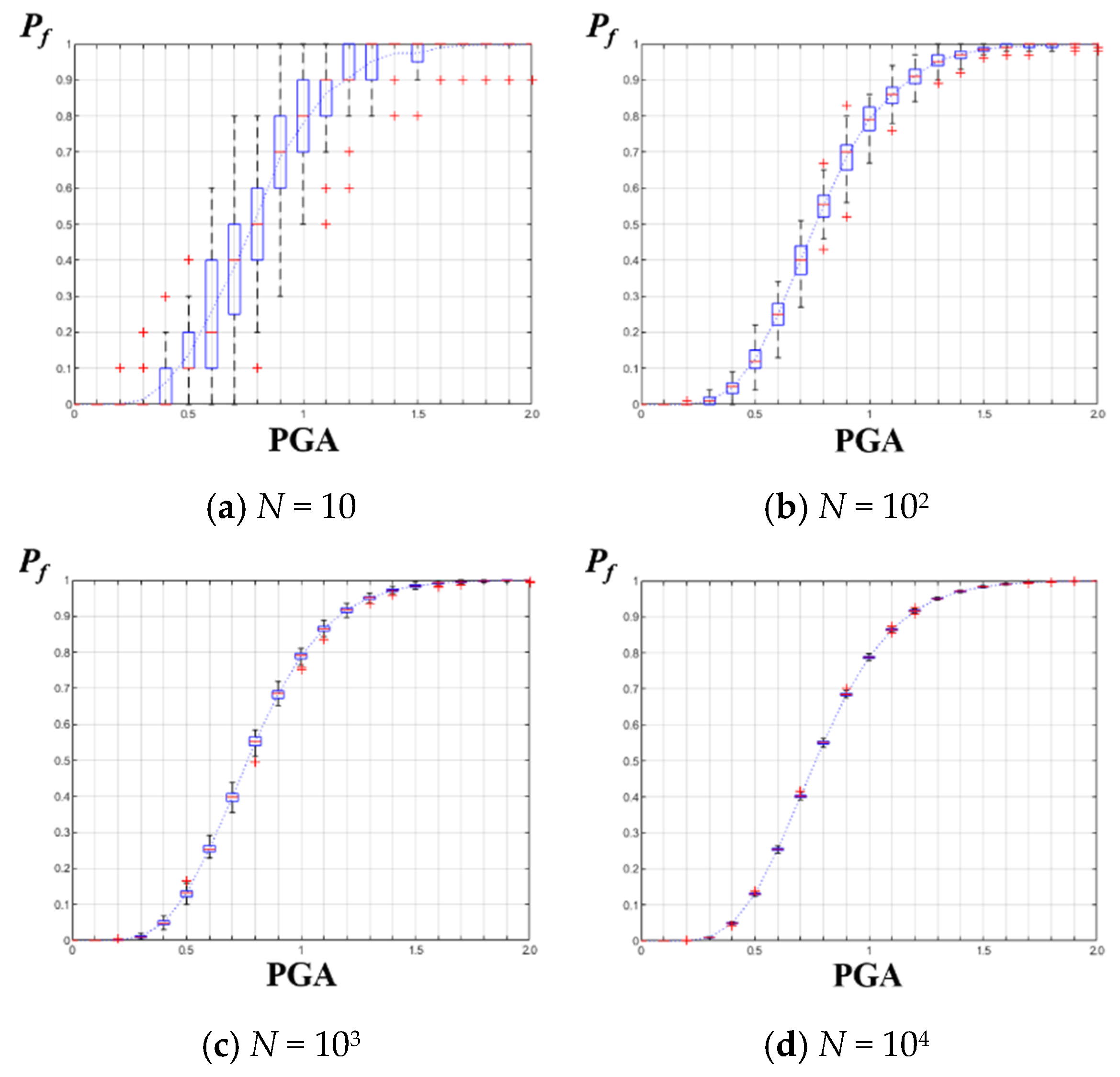
2.3. Performance of the Conventional DQFM

The conventional DQFM starts its process with the chosen N, and the same N is generated for all hazard conditions. Under the conventional DQFM algorithm, small N cannot be selected since the accuracy and the robustness of the final results depend on the N. For instance, boxplots of the results of single-hazard fragility analysis with different numbers of N are shown in Figure 2. It can be noticed in the failure probabilities for given peak ground accelerations (PGAs) that the variability of the results decreases as N increases. The results from a large N (e.g., 10⁴) indicate good convergence with small variability. Therefore, an alternative method that can reduce N yet provide the same performance as the conventional DQFM should be developed, while the conventional DQFM should use the large N to secure the convergence of the results.

3. Development of Two-Stage DQFM for Single- and Multi-Hazard Risk Quantification

For effective quantification of single- and multi-hazard risk to nuclear facilities, a two-stage DQFM is proposed in this section. To improve the computational efficiency of the conventional DQFM, this research aims to reduce the N without losing the accuracy or the robustness of the algorithm. When estimating single- and multi-hazard risk using DQFM, we found that the contribution of each hazard point to the final risk value varied by the hazard point. When the contribution of a certain point to the final risk is trivial, the difference between the probability of system failure estimated at that point from small N₁ and large N₂ could be negligible. For such hazard points, by using the small N₁ instead of large N₂ with less-significant hazard points, computational cost can be reduced.

With this inspiration, we developed a two-stage DQFM that generates a relatively small N₁ (e.g., 10²) for hazard points that make a small contribution to the final hazard risk, while generating large enough N₂ (e.g., 10⁴) for only those hazard points that make a large contribution to final risk. By dividing the hazard points by their contributions to the final risk value, the sampling cost that occurred in the hazard points that make a negligible contribution to the final risk value can be reduced. Since the purpose of the proposed method is to assign different Ns according to their contributions to the final system risk value, hazard points can be categorized into two or more groups (e.g., m-stage DQFM). However, we divided hazard points into only two groups to simplify the procedure and save the cost that occurred to divide the hazard groups. A flowchart of the two-stage DQFM is presented in Figure 3. The modified and extended modules that were first introduced in this paper are highlighted in blue.

In the first DQFM stage, a system failure probability is determined for all hazard points with a small N₁. system fragility curve is developed by the same procedure as the conventional DQFM. Later, hazard points are divided into two groups, and hazard points that have a non-negligible contribution to the final risk value are selected to be sampled again at the second DQFM stage with large N₂. To this end, “resampling rank” is assigned to hazard points. The resampling rank is the value that identifies the importance of each hazard point with respect to its contribution to the final risk. Once hazard points are divided into two groups, only the selected points are resampled in the second DQFM stage with a large N₂. Finally, the hazard risk of the system is determined by a convolution of the hazard information and the updated fragility curve.

The key process of the two-stage DQFM is to select hazard points, which will be updated in the second DQFM stage. The selection of these hazard points affects the accuracy and efficiency of the two-stage DQFM. In the following sub-sections, we describe the detailed process that we proposed to select the hazard points that have a non-negligible contribution to the final risk value.

3.1. Sorting Hazard Points

To identify the resampling points that make a non-negligible contribution to the final risk value, we employed two measures for each point as criteria: hazard information and risk information. It should be noted in Equations (3) and (4) that a large differential hazard value or risk value at a certain point indicates a large contribution to the final hazard risk. Therefore, to prioritize the hazard points by their importance, they are first sorted by their hazard and risk information. While differential hazard values can be determined by a given hazard map, risk information uses the results from the first DQFM stage. The risk value that is used to sort hazard points can be determined as follows:

$$Ris{k}_{single}\left(i\right)=F_1\left(i\right)\times dH\left(i\right)/dp$$

(7)

$$Ris{k}_{multi}\left(i,j\right)=F_1\left(i,j\right)\times dH\left(i,j\right)/dpdq$$

(8)

where F₁ is the approximated probability of system failure determined in the first DQFM stage. While the risk value itself contributes proportionally to the final risk value, a differential hazard value (see Equations (5) and (6)) can be considered as a weight of the error in the first DQFM stage. The results from the first stage, determined with a small N₁ (e.g., 10²), are expected to have high variability. The errors that occurred in this stage are convoluted with the hazard information, so they decrease the accuracy of the final risk. Since the error increases in proportion to the differential hazard value, the hazard points with large differential hazard values should be sampled again in the second DQFM stage to secure the accuracy of the final risk. Without including the hazard points with high differential hazard values, the accuracy of the final risk cannot be preserved.

3.2. Evaluating Cumulative Rates

After sorting the hazard points by their differential hazard and risk values in the first step, adequate threshold values are required to divide the points into two groups. The optimal threshold is expected to vary according to the diverse shapes of the system fragility curves. Therefore, rather than choose a certain value, we propose to use the cumulative rate as the threshold. The cumulative rate can represent the contribution of the hazard points as a group to the final risk value. The cumulative rate of the differential hazard value for single and multiple hazards at each point can be determined as follows:

$$H_{c,single}\left(a\right)={\displaystyle \sum }_{i^{*}=1}^{a}dH\left(i^{*}\right)/dp/{\displaystyle \sum }_{i^{*}=1}^{max}dH\left(i^{*}\right)/dp$$

(9)

$$H_{c,multi}\left(a\right)={\displaystyle \sum }_{i^{*}=1}^{a}dH\left(i^{*}\right)/dpdq/{\displaystyle \sum }_{i^{*}=1}^{max}dH\left(i^{*}\right)/dpdq$$

(10)

where H_c,single and H_c,multi are the cumulative rates of the differential hazard values for single and multiple hazards, respectively. i* is the newly given order that was achieved through the sorting process (Section 3.1), and a denotes the a^th order among the total hazard points of the single and multiple hazards. Similarly, the cumulative rate of the risk value for single and multiple hazards at each point can be determined as follows:

$$R_c\left(a\right)={\displaystyle \sum }_{i^{*}=1}^{a}Risk\left(i^{*}\right)/{\displaystyle \sum }_{i_s=1}^{max}Risk\left(i^{*}\right)$$

(11)

where R_c is the cumulative rate of the risk value of single and multiple hazards. For example, if H_c is 10⁻³, then the group of points lower than the hazard threshold contributed 0.1% to the total differential value of the hazard. As another example, if R_c is 10%, it means that the group of points lower than the risk threshold contributed 10% to the final risk value. By adopting this standard, the groups of points that make a trivial contribution to the final risk value can be identified.

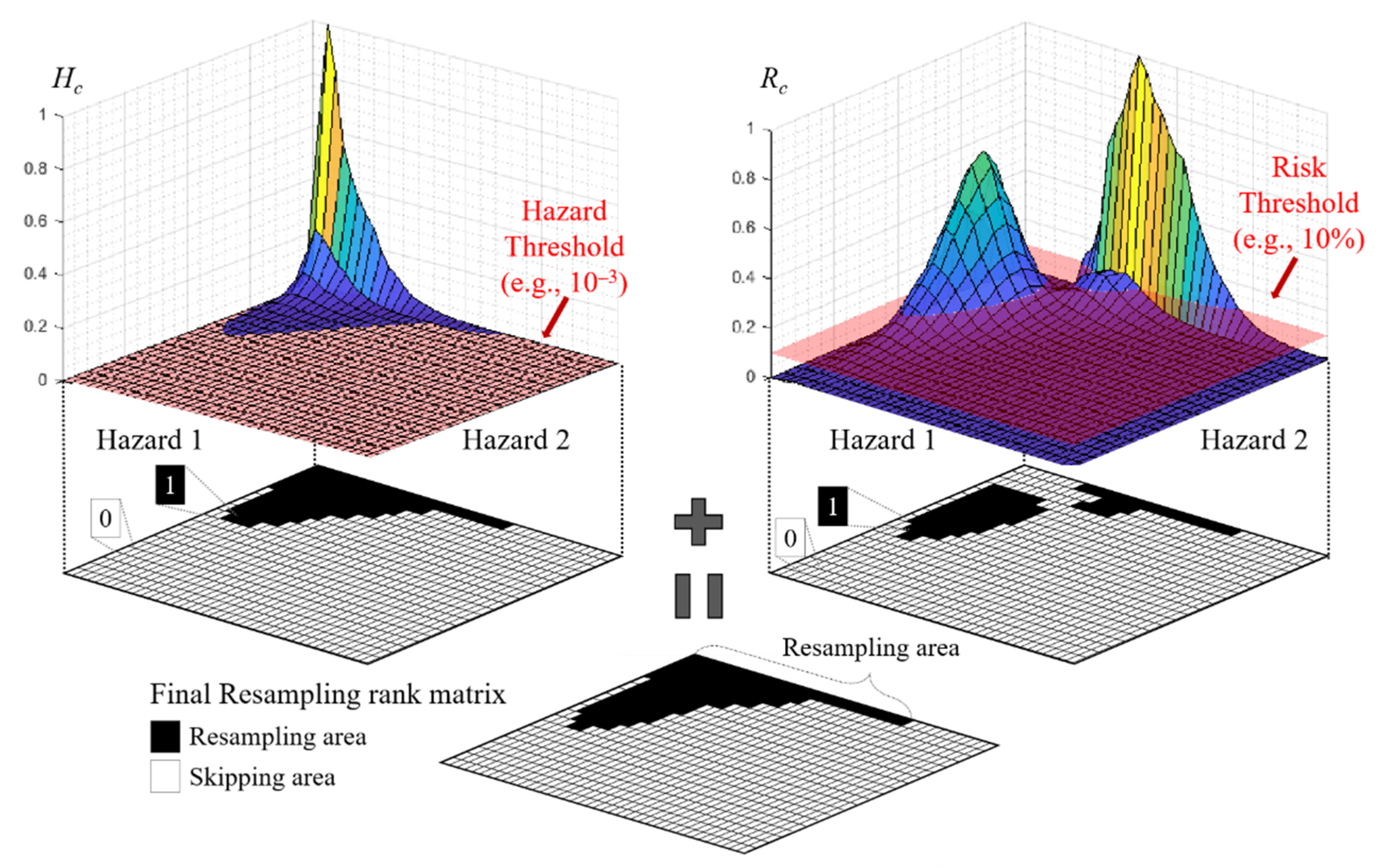
3.3. Selecting Threshold Values and Assigning the Resampling Rank

In the last step, the hazard points that make non-negligible contributions to the final risk or that have a large differential hazard value are selected as critical hazard points that need resampling in the second DQFM stage. Thus, one H_c value and one R_c value are selected as the thresholds (See Equations (9)–(11)). With the selected thresholds, we assign the binary “resampling rank” to each point in terms of Hc and Rc. For points smaller than the threshold, a resampling rank of 0 is assigned. For hazard points larger than the threshold, a resampling rank of 1 is assigned. Eventually, the combination of the critical points which were assigned a non-zero value is sampled again in the second DQFM stage.

Figure 4 and Figure 5 illustrate the assignment of resampling ranks for single and multiple hazards. They are expressed in a string and a matrix, respectively. It can be noticed in both figures that points with values smaller than the thresholds received the rank 0. After assigning the resampling rank according to the hazard and risk values (i.e., sub-system failures and total-system failure), the sum of the multiple strings (single hazard) or multiple matrices (multi-hazard) becomes the final resampling rank.

Subsequently, in the second DQFM stage, the points with non-zero resampling ranks are resampled with a large N₂ (e.g., 10⁴). The points that make a negligible contribution to the accuracy of the final risk value receive the resampling rank 0, and they are skipped in the second DQFM stage. Since the accuracy, robustness, and efficiency of the proposed method are subject to the threshold selection, choosing the optimal threshold is important. In Section 4 and Section 5, an extensive parametric study is presented to suggest the optimal thresholds for single- and multi-hazard risk quantification problems, respectively.

4. Single Hazard Example: Seismic Hazard

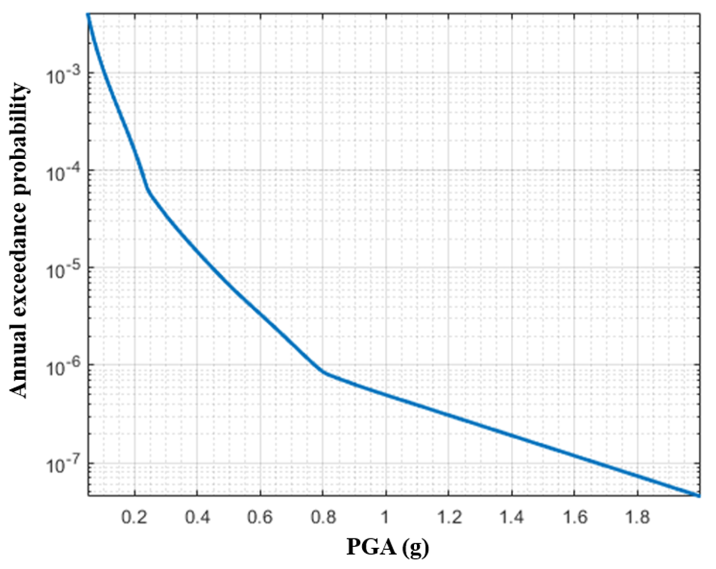
4.1. Setting the Problem

In this section, a two-stage DQFM is used to quantify the seismic risk to the Limerick Generating Station (LGS, Philadelphia, USA) NPP. The LGS NPP was selected to test the efficiency of the two-stage DQFM. To perform two-stage DQFM, hazard information, the system model, and the fragility model are required. First, the seismic hazard information from Kim et al. [17] is used (Figure 6), and the peak ground acceleration (PGA) from 0.05 to 2 g was uniformly divided into 196 hazard points. Second, the system model and the fragility information of the components were taken from Ellingwood [26]. The fragility information of each component is described in

Table 1. Seismic fragility and random failure probability information of Limerick Generating Station nuclear power plant (LGS NPP) components (adapted from Ref. [23]).

Component		Rms (Ams)	βRcs	ΒCcs	Mean Failure Rate (Per year)
S1	Offsite power	0.20 g	0.226	0.226	-
S2	Condensate storage tank	0.24 g	0.273	0.273	-
S3	Reactor internals	0.67 g	0.300	0.300	-
S4	Reactor enclosure structure	1.05 g	0.282	0.282	-
S6	Reactor pressure vessel	1.25 g	0.252	0.252	-
S10	Standby liquid control system tank	1.33 g	0.233	0.233	-
S11	440 V bus/steam generator breakers	1.46 g	0.411	0.411	-
S12	440 V bus transformer breaker	1.49 g	0.397	0.397	-
S13	125/250-V DC bus	1.49 g	0.397	0.397	-
S14	4 kV bus/steam generator	1.49 g	0.397	0.397	-
S15	Diesel generator circuit	1.56 g	0.368	0.368	-
S16	Diesel generator heat and vent	1.55 g	0.363	0.363	-
S17	Residual heat removal system heat exchangers	1.09 g	0.330	0.330	-
DGR	DGR—diesel generator common mode	-	-	-	0.00125
WR	WR—containment heat removal	-	-	-	0.00026
CR	CR—scram system mechanical failure	-	-	-	1.00 × 105
SLCR	SLCR—standby liquid control	-	-	-	0.01

, and the detailed sub-system failure scenarios of the LGS NPP are as presented in Equations (12)–(18).

$$A=S_{11}\cup S_{12}\cup S_{13}\cup S_{14}\cup S_{15}\cup S_{16}\cup D{G}_R$$

(12)

$$T_s{E}_{s}UX=S_{11}\cap A$$

(13)

$$T_s{R}_b=S_4$$

(14)

$$T_s{R}_{pv}=S_6$$

(15)

$$T_s{E}_s{C}_m{C}_2=S_1\cap \left(S_3{{\displaystyle \cup }}^{}{C}_R\right)\cap \left(A{{\displaystyle \cup }}^{}{S}_{10}{{\displaystyle \cup }}^{}SL{C}_R\right)$$

(16)

$$T_s{R}_b{C}_m=S_4{{\displaystyle \cap }}^{}\left(S_3\cup C_R\right)$$

(17)

$$T_s{E}_b{W}_m=S_1{{\displaystyle \cap }}^{}\overline{A}\cap \left(\left(\overline{S_{17}}\cap W_R\right){{\displaystyle \cup }}^{}\left(\overline{S_2}\cup S_{17}\right)\right)$$

(18)

The total-system failure scenario, or so-called core meltdown (CM), can be expressed as the union of all the sub-system failure scenarios (see Equations (13)–(18)), which can be simplified as follows:

$$CM=S_4{{\displaystyle \cup }}^{}{S}_6{{\displaystyle \cup }}^{}{S}_1{{\displaystyle \cap }}^{}\left[A\cup \left(S_3\cup C_R\right)\cap \left(S_{10}\cup SL{C}_R\right)\cap \left(S_{17}\cup W_R\right)\right]$$

(19)

Among the system components, four components, S11, S12, S13, and S14, in the same reactor building, and two components, S15 and S16, in the same diesel generator building, are assumed to be partially correlated because of their spatial adjacency. The correlation coefficient between the partially correlated components is assumed to be 0.7 (${\rho }_s=$ 0.7), while the other components are assumed to be independent.

As discussed in Section 3, two thresholds should be selected to perform the two-stage DQFM. Combinations of three hazard thresholds (i.e., 10⁻³, 10^−3.5, and 10⁻⁴, denoted by H3, H3.5, and H4, respectively) and six risk thresholds (i.e., 100%, 30%, 20%, 10%, 5%, and 1%, denoted by R100, R30, R20, R10, R5, and R1, respectively) are investigated to identify the optimal combination of thresholds. For instance, the H3R10 threshold means that any point which has an H_c larger than 10⁻³ or an R_c larger than 10% is resampled in the second DQFM stage with large N₂.

Lastly, to perform conventional DQFM and the two-stage DQFM, the number of sample N and sampling method must be defined. The conventional DQFM generated N = 10⁴ samples for all hazard points, while the two-stage DQFM generated N₁ = 10² and N₂ = 10⁴ samples for the first and second DQFM stages, respectively. In terms of the sampling method, both the conventional DQFM and the proposed two-stage DQFM used MCS to generate the samples. To investigate the variability of the two-stage DQFM due to MCS, every condition is performed 500 times, which is sufficient value based on test run. The numerical investigations were conducted by MATLAB code using a personal computer with Windows 10 (64 bit) operating system equipped with an Intel(R) Core(TM) i7-9700K CPU @ 3.6 GHz and 16 GB RAM.

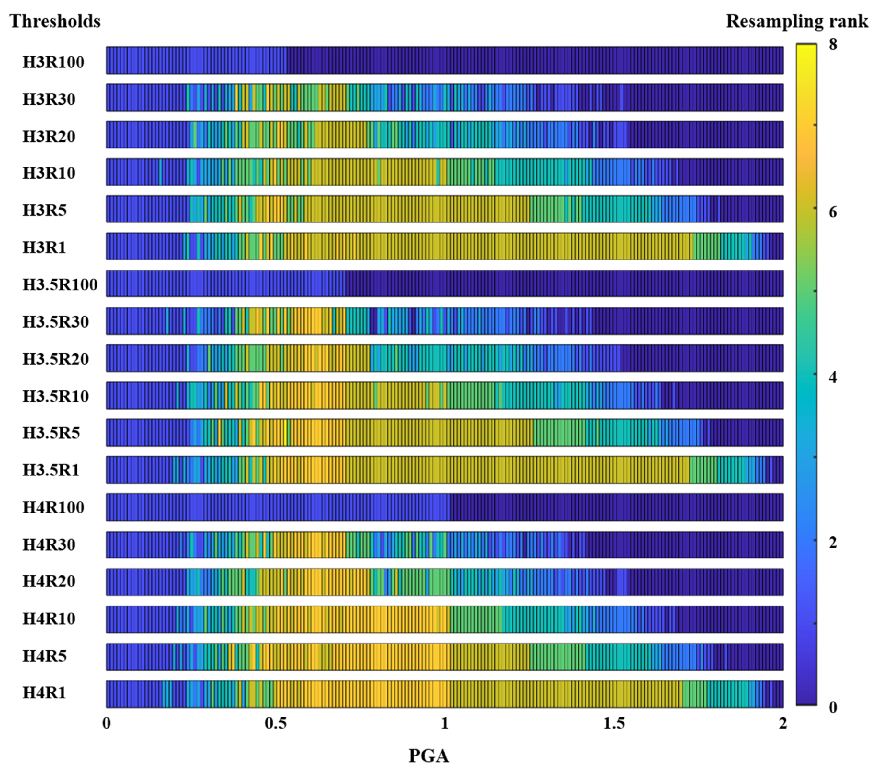
4.2. Results and Discussion

Figure 7 shows the resampling points selected by the proposed two-stage DQFM with 18 thresholds. Each result was achieved by a single run of the proposed two-stage DQFM, and the colors represent the resampling rank of each hazard point. It should be noted that high PGAs are more likely than small PGAs to have a resampling rank of zero. So, they make a negligible contribution to the final risk value, and they are skipped in the second DQFM stage. The two-stage DQFM selects diverse resampling hazard points based on the threshold selection. As a result, the accuracy, results, and computational efficiency of the algorithm vary by the threshold selection.

In addition, to show the difference between the proposed DQFM and conventional DQFM, the system fragility curves from both approaches are compared in Figure 8. The system fragility curves from two-stage DQFM are not as smooth as those from the conventional DQFM at points that are larger than 1.4 g, since the results from the two-stage DQFM were achieved with a small N₁. The difference between the two fragility curves occurred only at the points that made a small contribution to the final risk value. Therefore, the accuracy of the final result was not affected by the gaps in the fragility curves. To validate the accuracy and the robustness of the proposed method, despite the rougher system curve shown in Figure 8, 500 different sample sets were generated for each threshold condition. The means and the standard deviations of the 500 sets of results, the average Ns, and the computational costs of the conventional and the two-stage DQFM with various thresholds were compared.

First, to investigate the accuracy of the proposed method, the normalized means of the 500 sets of the failure risk values of sub-systems and the total system (See Equations (13)–(19)) were determined. The results for the 500 sets from the two-stage DQFM were divided by those from the conventional DQFM. The results in Figure 9 show that there was little difference between the risk values from the conventional and the proposed methods. Besides the T_sE_sW_m scenario (“▷” mark in Figure 9), the two-stage DQFM with the most threshold conditions showed good agreement—less than 0.5% difference—with the conventional DQFM.

After validating the accuracy of the proposed method, the robustness and the efficiency of the algorithm were also examined by comparing the variability of the results and the corresponding resampling ratios. For each sub-system and total-system failure scenario, the standard deviation of the 500 results from the two-stage DQFM was divided by that from the conventional DQFM. Later, the mean of the normalized standard deviations was determined as follows:

$$\frac{\overline{{\sigma }_{TS}}}{\overline{{\sigma }_{DQFM}}}=\frac{{{\displaystyle \sum }}_{i=1}^{k+1}{\sigma }_{i,TS}/{\sigma }_{i,DQDM}}{k+1}$$

(20)

where $\overline{{\sigma }_{TS}}$ and $\overline{{\sigma }_{DQFM}}$ are the means of σ_i,TS and σ_i,DQFM, and these denote the standard deviations of the i^th failure scenario by the two-stage DQFM and the conventional DQFM, respectively. k is the number of sub-system failure scenarios (see Equations (13)–(19)). In addition, the ratio of resampling points was computed as follows:

$$resampling points ratio=\frac{resampling points}{number of hazard points}$$

(21)

In this example, the number of hazard points is 196. Figure 10 presents the mean of normalized standard deviations and resampling ratios from the two-stage DQFM with different thresholds. The balance between the number of samples and the performance of the two-stage DQFM can be indicated in this figure. In general, the two-stage DQFM with any threshold conditions that have a resampling ratio higher than 70% delivered a variability similar to that from the conventional DQFM. Especially, consideration of accuracy, variability, and efficiency, the H4R30 condition is suggested as the optimal threshold for a single-hazard risk assessment with the two-stage DQFM.

The detailed results determined by conventional DQFM and two-stage DQFM with H3R30 threshold are presented in

Table 2. Results of 500 sets of seismic risk to the LGS NPP using the conventional DQFM and the two-stage DQFM.

System Failure Scenario	DQFM		Two-stage DQFM *
	μ	σ	μ	σ
TsEsUX	2.57 × 106	2.16 × 108	2.57 × 106	1.95 × 108
TsRb	1.14 × 106	6.31 × 109	1.14 × 106	6.33 × 109
TsRpv	4.96 × 107	2.01 × 109	4.94 × 107	2.22 × 109
TsEsCmC2	1.17 × 106	7.29 × 109	1.17 × 106	7.32 × 109
TsRbCm	6.65 × 107	2.46 × 109	6.64 × 107	2.52 × 109
TsEsWm	1.13 × 107	3.79 × 108	1.15 × 107	3.80 × 108
CM	4.32 × 106	4.34 × 108	4.32 × 106	4.41 × 108
Average Ns **	196 × 2 × 104		First stage Second stage Total	196.00 × 2 × 102 135.71 × 2 × 104 137.67 × 2 × 104
Total computation time	529.0 s		424.5 s

* Results with the H4R30 threshold. ** Average number of samples generated for each component.

. The means, standard deviations, and the average Ns show that the two-stage DQFM used only 70% of the samples from the conventional DQFM while delivering similar accuracy and variability. Also, the computational times required for conventional DQFM and the two-stage DQFM with the H4R30 condition were about 529.0 and 424.5 s, respectively. This improvement in performances proves that the proposed two-stage DQFM is effective even when the number of generated samples is smaller than conventional DQFM.

Saving approximately 20% of the computational time in a single-hazard risk quantification problem might seem trivial, and may not have the advantage when risk quantification is performed for a single time. yet it can be an important difference when repeated hazard risk quantifications are required (e.g., system maintenance optimization problem [27] which uses the system risk value as one of the objective functions [28]). Moreover, computational cost reduction during single-hazard risk quantification means that further computational costs can be reduced in the higher dimension (i.e., multiple hazards). Therefore, the efficiency of the two-stage DQFM in multi-hazard risk quantification is investigated in Section 5.

5. Multi-Hazard Example: Earthquake and Tsunami

5.1. Setting the Problem

To further examine the benefit of using two-stage DQFM for risk quantification, a multi-hazard example, the LGS NPP under earthquake–tsunami hazard, was investigated. The earthquake–tsunami hazard information was taken from a report by the Korea Atomic Energy Research Institute (KAERI) [29]. As shown in Figure 11, the seismic intensity (PGA, g) was uniformly divided into 21 points, and the tsunami intensity (inundation depth, m) was uniformly divided into 41 points. Accordingly, the final multi-hazard grid has 861 points. While the same system model and seismic fragility model were adopted (See Equations (13)–(19) and Table 1), tsunami fragility information is adopted from Kwag et al. [23] and summarized in

Table 3. Tsunami fragility of the LGS NPP components (adapted from Ref. [23]).

Component		Rmt (Amt)	βRct	ΒCct
S1	Offsite power	10 m	0.354	0.354
S2	Condensate storage tank	10 m	0.212	0.212
S11	440 V bus/SG * breakers	11 m	0.212	0.212
S12	440 V bus transformer breaker	11 m	0.212	0.212
S13	125/250 V DC ** bus	11 m	0.212	0.212
S14	4 kV bus/SG	11 m	0.212	0.212
S15	Diesel generator circuit	11 m	0.212	0.212
S17	RHR *** heat exchangers	10 m	0.212	0.212

* Steam generator. ** Direct current. *** Residual heat removal.

. Like the previous example, two groups of components are assumed to be partially correlated because of spatial proximity (${\rho }_s={\rho }_t=$ 0.7): S11, S12, S13, and S14 are in the same reactor building, and S15 and S16 are located in the same diesel generator building.

To perform two-stage DQFM, the 18 threshold combinations used in the single hazard risk assessment are used. The two-stage DQFM with various thresholds and the conventional DQFM are compared using the means and standard deviations of the results from 500 sets of evaluation, the number of total samples, and computation time. Also, this example adopts same options, i.e., N = 10⁴ for conventional DQFM, and N₁ = 10² and N₂ = 10⁴ for two-stage DQFM. The numerical investigations were conducted using a personal computer with Windows 10 (64 bit) operating system equipped with an Intel(R) Core(TM) i7-9700K CPU @ 3.6 GHz and 16 GB RAM.

5.2. Results and Discussion

Figure 12 shows the resampling points selected by a single run of the proposed two-stage DQFM with 18 thresholds. It should be noted that the resampling ratio varies by the threshold selection, and hazard points with high PGAs or high inundation depth were more likely to have a resampling rank of zero, while those with low values had a resampling rank of one. The two-stage DQFM selected diverse resampling hazard points based on the threshold selection, which affects the accuracy and the computational efficiency of the algorithm.

In addition, the system fragility curves from the conventional DQFM and the two-stage DQFM with H3.5R20 and H4R1 thresholds are compared in Figure 13 with their corresponding resampling ranks. Figure 13a shows that the system fragility curve of the two-stage DQFM was not as smooth as that from the conventional DQFM because there were very few resampling points. On the other hand, Figure 13b shows that a smoother system fragility curve can be achieved with a larger number of resampling points. As Figure 13a,b show, the number of resampling points and the convergence of the system fragility curve have a tradeoff relationship. To validate the two-stage DQFM and to find the most efficient combination of thresholds, results from 500 different sets were further investigated by each approach and threshold.

First, to validate the accuracy of the results, the means of the multi-hazard risks from the two-stage DQFM were compared with that of the conventional DQFM. The normalized means of 500 sets, which divided the results from the two-stage DQFM by the conventional DQFM, are plotted in Figure 14. In general, the results from the two-stage DQFM show a high level of accuracy. There is less than a 0.5% difference from the results from the conventional DQFM. The results from the T_sE_sW_m (“▷” mark in Figure 14) failure scenario have a relatively larger difference than other scenarios, yet still show the good agreement between the two approaches regardless of the threshold selection.

Second, to validate the efficiency of the two-stage DQFM, the mean of normalized standard deviations (See Equation (20)) was determined and plotted in Figure 15 with the corresponding resampling ratio. Results show the tradeoff between the number of resampling points and the standard deviation at the Pareto surface. As the resampling ratio increases, the mean of normalized standard deviations converges toward 1, which means that the variabilities of the two approaches are the same. Among the threshold combinations, H3.5R20 was identified as the optimal threshold; there is little benefit of increasing resampling points larger than H3.5R20. Including the H3.5R20 threshold, most of the threshold combinations with a resampling ratio higher than 20% show the similar or less variability than that of the conventional DQFM.

Table 4. Results of 500 sets of earthquake-tsunami risk scenarios at the LGS NPP using the conventional DQFM and the two-stage DQFM.

System Failure Scenario	DQFM		Two-Stage DQFM *
	μ	σ	μ	σ
TsEsUX	5.53 × 106	3.62 × 108	5.53 × 106	3.67 × 108
TsRb	1.04 × 106	5.84 × 109	1.04 × 106	5.65 × 109
TsRpv	4.10 × 107	2.24 × 109	4.10 × 107	2.41 × 109
TsEsCmC2	1.10 × 106	6.71 × 109	1.10 × 106	6.92 × 109
TsRbCm	5.83 × 107	2.73 × 109	5.83 × 107	2.82 × 109
TsEsWm	8.51 × 107	2.84 × 108	8.50 × 107	2.83 × 108
CM	8.20 × 106	4.63 × 108	8.21 × 106	4.72 × 108
Average Ns **	861 × 4 × 1× 104		First stage Second stage Total	861.00 × 4 × 102 175.47 × 4 × 104 184.08 × 4 × 104
Total computation time	3128.5 s		862.9 s

* Results with the H3R30 threshold. ** Average number of samples generated for each component.

summarizes the means and the standard deviations of the sub-systems and total-system risks determined by the conventional DQFM and the two-stage DQFM with the H3.5R20 threshold. The computational time required for conventional DQFM and the two-stage DQFM with the H3.5R20 condition was about 3128.5 s and 862.9 s, respectively. The two-stage DQFM required about 28% of the computational time needed by the conventional DQFM, yet it did not lose the accuracy and variability of the results.

A comparison of the results of the single- and multi-hazard examples (Section 4 and Section 5) shows that the efficiency of the two-stage DQFM is more notable for risk assessment with multiple hazards than with a single hazard. The efficiency of the developed method disproportionally increases for higher dimensions since the resampling ratio quickly decreases as the hazard dimension increases. It could be expected from this result that the two-stage DQFM can further increase computational efficiency for multi-hazard situations with more than two hazards. Such computational benefits of the two-stage DQFM would contribute to multi-hazard risk reduction by allowing multi-hazard risk planning with reduced computational costs.

6. Conclusions

This paper proposed a two-stage DQFM method to improve the computational efficiency of the conventional DQFM method without losing the accuracy or variability of the results. To this end, the two-stage DQFM divides the hazard points into two groups based on their contribution to the final hazard risk values, and it assigns a different number of samples to each group. Two measures (i.e., the cumulative rate of the differential hazard value and the risk value) were adopted to classify the hazard points by their importance. The validity and the improved efficiency of the two-stage DQFM were demonstrated using both single- and multi-hazard risk assessment problems. Especially in the multi-hazard risk quantification problem, the proposed method showed a significant reduction of computational cost: it required only 28% of the cost of the conventional DQFM. As a result, the proposed method is expected to support single- and multi-hazard risk quantification of nuclear facilities with improved computational efficiency.

References

1. Yang, J.E. Fukushima Dai-Ichi accident: Lessons learned and future actions from the risk perspectives. Nucl. Eng. Technol. 2014, 46, 27–38. [Google Scholar] [CrossRef] [Green Version]
2. Tsuboi, S.; Mine, T.; Kanke, S.; Ohira, T. Who needs care? The long-term trends and geographical distribution of deaths due to acute myocardial infarction in Fukushima Prefecture following the Great East Japan Earthquake. Int. J. Disaster Risk Reduct. 2019, 41, 101318. [Google Scholar] [CrossRef]
3. Choi, E.; Ha, J.; Hahm, D.; Kim, M. A Review of Multihazard Risk Assessment: Progress, Potential, and Challenges in the Application to Nuclear Power Plants. Int. J. Disaster Risk Reduct. 2020, 101933. [Google Scholar] [CrossRef]
4. Ebisawa, K.; Fujita, M.; Iwabuchi, Y.; Sugino, H. Current issues on PRA regarding seismic and tsunami events at multi units and sites based on lessons learned from Tohoku earthquake/tsunami. Nucl. Eng. Technol. 2012, 44, 437–452. [Google Scholar] [CrossRef]
5. Reed, J.W.; Kennedy, R.P. Methodology for Developing Seismic Fragilities; EPRI TR-103959; Electric Power Research Institute: Palo Alto, CA, USA, 1994. [Google Scholar]
6. Hur, J.; Shafieezadeh, A. Multi-hazard probabilistic risk analysis of off-site overhead transmission systems. In Proceedings of the 25th Conference on Structural Mechanics in Reactor Technology, SMiRT25, Charlotte, NC, USA, 4–9 August 2019. [Google Scholar]
7. Mun, C.U. Bayesian Network for Structures Subjected to Sequence of Main and Aftershocks. Master’s Thesis, Seoul National University, Seoul, Korea, 2019. [Google Scholar]
8. Ryu, H.; Luco, N.; Uma, S.R.; Liel, A.B. Developing fragilities for mainshock-damaged structures through incremental dynamic analysis. In Proceedings of the Ninth Pacific Conference on Earthquake Engineering, Auckland, New Zealand, 14–16 April 2011. [Google Scholar]
9. Salman, A.M.; Li, Y. A probabilistic framework for multi-hazard risk mitigation for electric power transmission systems subjected to seismic and hurricane hazards. Struct. Infrastruct. Eng. 2018, 14, 1499–1519. [Google Scholar] [CrossRef]
10. Prabhu, S.; Javanbarg, M.; Lehmann, M.; Atamturktur, S. Multi-peril risk assessment for business downtime of industrial facilities. Nat. Hazards 2019, 97, 1327–1356. [Google Scholar] [CrossRef]
11. Prabhu, S.; Ehrett, C.; Javanbarg, M.; Brown, D.A.; Lehmann, M.; Atamturktur, S. Uncertainty Quantification in Fault Tree Analysis: Estimating Business Interruption due to Seismic Hazard. Nat. Hazards Rev. 2020, 21, 04020015. [Google Scholar] [CrossRef]
12. Leverenz, F.L.; Kirch, H. User’s Guide for the WAM-BAM Computer Code; No. PB--249624; Science Applications. Inc.: Palo Alto, CA, USA, 1976. [Google Scholar]
13. Bohn, M.P.; Shieh, L.C.; Wells, J.E. Application of the SSMRP Methodology to the Seismic Risk at the Zion Nuclear Power Plant; No. NUREG/CR—3428; Lawrence Livermore National Lab.: Fermore, CA, USA, 1983. [Google Scholar]
14. Watanabe, Y.; Oikawa, T.; Muramatsu, K. Development of the DQFM method to consider the effect of correlation of component failures in seismic PSA of nuclear power plant. Reliab. Eng. Syst. Saf. 2003, 79, 265–279. [Google Scholar] [CrossRef]
15. Li, J. Fault-Event Trees Based Probabilistic Safety Analysis of a Boiling Water Nuclear Reactor’s Core Meltdown and Minor Damage Frequencies. Safety 2020, 6, 28. [Google Scholar] [CrossRef]
16. EPRI. Seismic Fragility Application Guide; TR-1002988; Electric Power Research Institute: Palo Alto, CA., USA, 2002. [Google Scholar]
17. Kim, J.H.; Choi, I.-K.; Park, J.-H. Uncertainty analysis of system fragility for seismic safety evaluation of NPP. Nucl. Eng. Design 2011, 241, 2570–2579. [Google Scholar] [CrossRef]
18. Kwag, S.; Oh, J.; Lee, J.M.; Ryu, J.S. Bayesian based seismic margin assessment approach: Application to research reactor system. Earthq. Struct. 2017, 12, 653–663. [Google Scholar]
19. Zhou, T.; Modarres, M.; Droguett, E.L. Issues in dependency modeling in multi-unit seismic PRA. In Proceedings of the International Topical Meeting on Probabilistic Safety Assessment (PSA 2017), American Nuclear Society, Pittsburgh, PA, USA, 24–28 September 2017. [Google Scholar]
20. Budnitz, R.J.; Hardy, G.S.; Moore, D.L.; Ravindra, M.K. Correlation of Seismic Performance in Similar SSCs (Structures, Systems, and Components); No. NUREG/CR-7237; US Nuclear Regulatory Commission: Rockville, MD, USA, 2017. [Google Scholar]
21. Kaplan, S. A Method for handling dependency and partial dependency of fragility curve in seismic risk quantification. In Transactions SMiRT 8 Int. Conf.; IASMiRT: Brussels, Belgium, 1985; Volume M, pp. 595–600. [Google Scholar]
22. Kim, J.H.; Kim, S.Y.; Choi, I.K. Combination Procedure for Seismic Correlation Coefficient in Fragility Curves of Multiple Components. J. Earthq. Eng. Soc. Korea 2020, 24, 141–148. [Google Scholar] [CrossRef]
23. Kwag, S.; Ha, J.G.; Kim, M.K.; Kim, J.H. Development of Efficient External Multi-Hazard Risk Quantification Methodology for Nuclear Facilities. Energies 2019, 12, 3925. [Google Scholar] [CrossRef] [Green Version]
24. Kwag, S.; Eemb, S.; Choi, E.; Ha, J.G.; Hahm, D. Toward Improvement of Sampling-based Seismic Probabilistic Safety Assessment Method for Nuclear Facilities. Reliab. Eng. Syst. Saf. Under review.
25. Aksoy, A.; Martelli, M. Mixed partial derivatives and Fubini’s theorem. Coll. Math. J. 2002, 33, 126–130. [Google Scholar] [CrossRef]
26. Ellingwood, B. Validation studies of seismic PRAs. Nucl. Eng. Des. 1990, 123, 189–196. [Google Scholar] [CrossRef]
27. Choi, E.; Song, J. Cost-effective retrofits of power grids based on critical cascading failure scenarios identified by multi-group non-dominated sorting genetic algorithm. Int. J. Disaster Risk Reduct. 2020, 49, 101640. [Google Scholar] [CrossRef]
28. Kwag, S.; Hahm, D. Multi-objective-based seismic fragility relocation for a Korean nuclear power plant. Nat. Hazards 2020, 103, 3633–3659. [Google Scholar] [CrossRef]
29. KAERI. Development of Site Risk Assessment & Management Technology including Extreme External Events; KAERI/RR-4225/2016; Korea Atomic Energy Research Institute: Daejeon, Korea, 2017. [Google Scholar]
Figure 1. Flowchart of the conventional direct quantification of fault tree using Monte Carlo simulation (DQFM) for single- and multi-hazard risk quantification (adapted from Ref. [14,23]).
Energies 14 01017 g001
Figure 2. The variability of seismic fragility curves by the conventional DQFM for various Ns: (a) N = 10, (b) N = 102, (c) N = 103, (d) N = 104.
Energies 14 01017 g002
Figure 3. Flowchart of the proposed two-stage DQFM for single- and multi-hazard risk quantification.
Energies 14 01017 g003
Figure 4. Illustration of the assignment of resampling ranks for a single-hazard example.
Energies 14 01017 g004
Figure 5. Illustration of the assignment of resampling ranks for a multi-hazard example.
Energies 14 01017 g005
Figure 6. Seismic hazard information for the LGS NPP (adapted from Ref. [17]).
Energies 14 01017 g006
Figure 7. Resampling ranks of the single-hazard example from a single run of the two-stage DQFM.
Energies 14 01017 g007
Figure 8. System fragility curves of the single-hazard example using the conventional and two-stage DQFM with H3R30 threshold.
Energies 14 01017 g008
Figure 9. Comparison of the accuracy of using the normalized means of 500 sets of seismic risk to the LGS NPP from various thresholds.
Energies 14 01017 g009
Figure 10. Efficiency comparison using the mean of the normalized standard deviations of 500 sets of the seismic risk of the LGS NPP from various thresholds.
Energies 14 01017 g010
Figure 11. Earthquake–tsunami hazard curve for the LGS NPP (adapted from Ref. [29]).
Energies 14 01017 g011
Figure 12. Resampling ranks of multi-hazard example by a single run of the two-stage DQFM.
Energies 14 01017 g012
Figure 13. Earthquake–tsunami fragility curves for the LGS NPP using the conventional DQFM and the two-stage DQFM with (a) H3.5R20 and (b) H4R1 thresholds.
Energies 14 01017 g013
Figure 14. Comparison of the accuracy of using the normalized means of 500 sets of earthquake–tsunami risk to the LGS NPP from various thresholds.
Energies 14 01017 g014
Figure 15. Comparison of efficiency using the mean of the normalized standard deviations of 500 sets of earthquake–tsunami risk to the LGS NPP from various thresholds.
Energies 14 01017 g015