1. Introduction
An increased awareness of the need for a carbon neutral energy production has led to a corresponding increase in biomass combustion. The world’s primary energy consumption in 2019 amounted to 584 EJ of which coal constituted 27% and renewables (including biofuel) to 5%. In the European Union, the numbers are 69 EJ, 11%, and 11%, respectively [
1]. Combustion of biomass can be regarded as a carbon neutral source for energy [
2]. Coal releases approximately 93
tons CO
/EJ, depending on coal type and origin [
3,
4]. Byutilizing suspension firing technology in existing coal power plants rebuilt to combust biomass particles, a decrease in carbon emissions can be obtained, which enables the European Union’s Green deal of no net emission of green house gasses by 2050. In combined heat and power plants, up to 90% of the energy stored in woody biomass can be recovered as heat and electricity [
2]. Thus, with this aim, the interest in retrofitting suspension firing units to combust biomass instead of coal has increased over the past decades. Suspension firing of biomass is typically done with small particle sizes (
= 0.1–3 mm), [
5] at high temperatures (
T > 1000 K), [
6], and at high heating rates (>10
–10
K/s) [
7].
In order to predict biomass flame behavior and boiler chamber conditions, modeling of biomass suspension firing is used [
8,
9]. A reasonably accurate representation of the devolatilization process is crucial in obtaining correct modeling results. Flame characterization and, consequently, flame attachment to the burner quarl in full sized industrial burners is dependent on the time for onset of devolatilization and the amount of volatiles released [
8]. A better flame characterization will allow for higher fuel flexibility and plant efficiency. These challenges can be investigated through CFD combustion modeling.
Modeling a suspension firing unit often involves CFD simulations [
10]. To avoid too high computational costs, subprocesses in the particle combustion modeling in CFD require simplifications. Coal particles have historically been modeled as isothermal in CFD combustion simulations, and this approach has sometimes been extended to also include modeling of biomass pyrolysis [
11,
12,
13]. However, model work validated against experimental data [
14,
15] shows that biomass particles at sizes and temperatures relevant for suspension firing cannot be regarded as thermally thin, i.e., isothermal. Some thermally thick particle conversion models exists in CFD focusing on efficient use of computational power [
16,
17], which with some limitations adequately predicts biomass devolatilization at fluidized and fixed bed conditions. More complicated particle models are not feasible in CFD for industrial modeling purposes, due to high computational costs [
9].
Simplified devolatilization models [
9,
15,
18], which account for the complicated process of biomass devolatilization in a simple lumped fashion, have previously been presented. In these isothermal models, apparent devolatilization kinetic parameters have included heat transfer limitations, which were not otherwise included. None of the models, however, take the effect of biomass density, gas temperature, or particle morphology into account. These are important properties, influencing flame stability and onset of devolatilization.
To compromise between the need for a simple devolatilization model and the need for describing the complicated phenomenon of biomass particle pyrolysis, this paper introduces lumped Arrhenius kinetic parameters for a single first order global pyrolysis model. The parameters of a zero dimensional, isothermal model are found by fitting to predictions of a semi-two dimensional model [
19] that previously has been validated against experimental data. The comparison is done for different gas temperatures, particle sizes, particle aspect ratios, and densities. The combined effect of these experimental properties on the Arrhenius parameters is quantified using the multivariate data analysis method, partial least squares regression (PLS). To the knowledge of the authors, no experimental data valid for suspension firing of woody biomass exist, which has not been used in the development of the semi-two dimensional model. Thus, the present model is not directly evaluated further against experimental data.
2. Method and Model Description
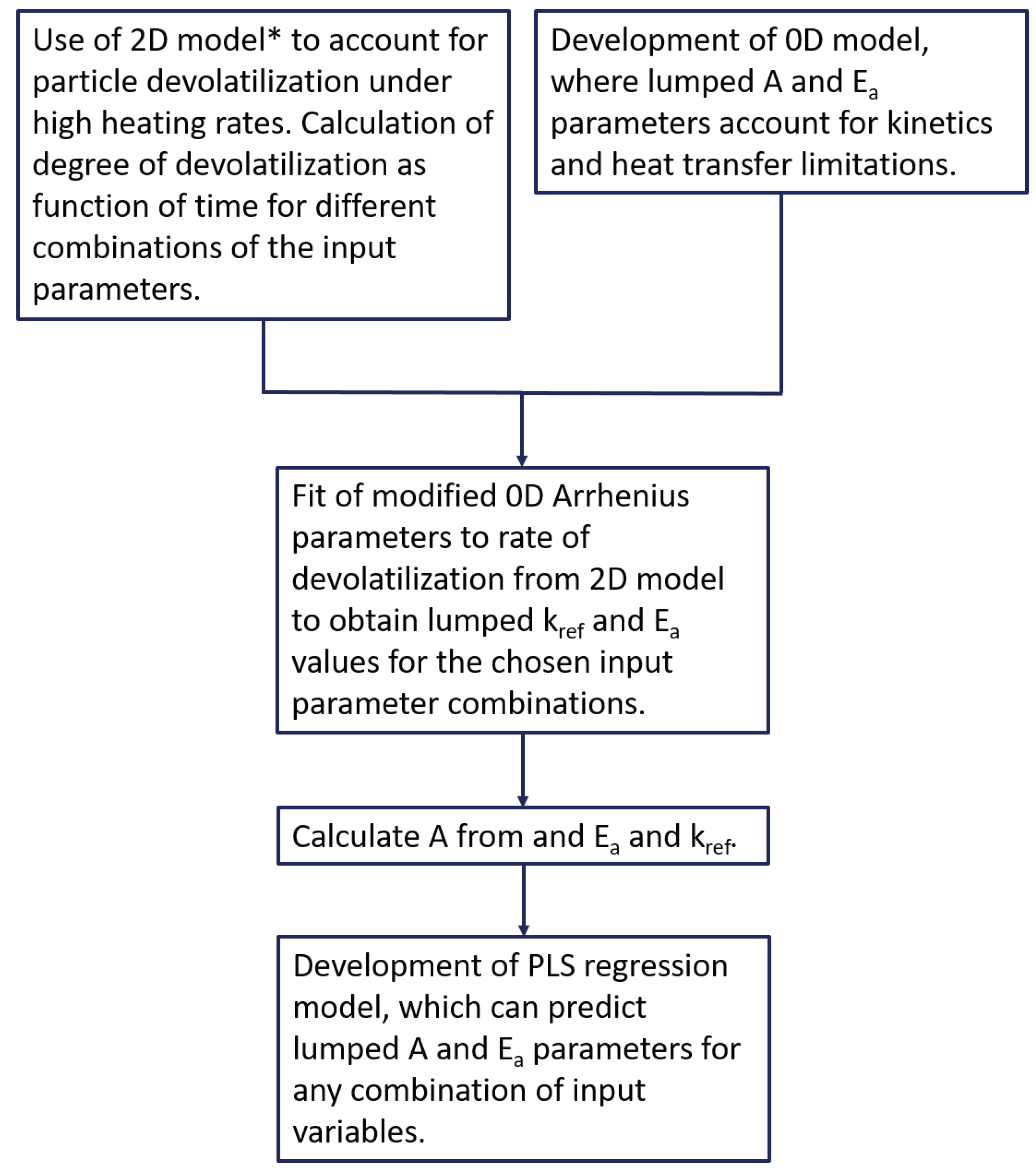
The model development process is done in two parallel tracks, which are subsequently compared and used for final model determination. An overview can be seen in
Figure 1. In a previously published paper, a rigorous semi-2D model was developed [
19]. In this paper, a 0D model is set up. Subsequently the lumped 0D Arrhenius parameters,
A and
E, which provide the best agreement between the 0D and the semi-2D model for a range of selected cases are determined. Then, a PLS model is established, which calculates the lumped Arrhenius parameters from particle radius, aspect ratio, particle density, and maximum gas temperature. The model development process is described in more detail in the subsequent sections.
2.1. The Semi-Two Dimensional Model
The semi-two dimensional model is described in detail elsewhere [
19,
20,
21], and only a short introduction will be given here. The model was first presented for devolatilization at medium heating rates by Thunman et al. [
20], and subsequently developed further by Ström and Thunman [
21]. It was recently adapted to account for biomass devolatilized under suspension firing conditions by Leth-Espensen et al. [
19]. The model is a shell model capable of describing both cylindrical and spherical geometries. The cylinder is the preferred simple geometry to model biomass particles, [
22] whereas coal particles tend to be almost spherical in nature. The cylindrical model takes changes during devolatilization in both radius and length into account using one variable only. The decrease in particle length is assumed comparable to the decrease in radius, thus particle shrinking is described only by the radius. Overall, the cylindrical model accounts for the internal temperature gradient, the volume, and surface area in two dimensions, whereas the heat transfer is solved in a one dimensional manner. The spherical model is one dimensional. Regardless of the shape, in the model, the particle is divided into three concentric shells. The innermost layer consists of moist biomass, the middle layer is dry biomass, and the outer layer is char. The shells move inwards during the devolatilization, transforming the model particle from consisting of practically only a moist shell in the beginning to be all char after full devolatilization. The model accounts for intraparticle heat and mass transfer.
2.2. The Zero Dimensional Model
The 0D model is based on the following assumptions:
The particle is isothermal.
The particle has constant density (shrinking particle).
The particle is dry.
The particle is spherical.
The initial particle diameter,
R, is defined as the initial cylinder diameter, according to recommendations in [
19].
The devolatilization enthalpy is assumed to be 0.
Both the influences of kinetics and heat transfer are described by a single first order reaction model.
The wall radiation temperature is defined as − 200 K.
The devolatilization process in the isothermal particle is modeled as a global reaction, using the single first order reaction (SFOR) model, described in Equation (
1) [
23].
Here,
t is the time,
is the fraction of volatiles released,
is the fraction of volatiles present in the particle at
t = 0, and
k is an Arrhenius reaction rate constant given in Equation (
2).
is the gas constant,
T is the particle temperature, and
A and
E are the Arrhenius pre-exponential factor and activation energy, respectively. The temperature in the particle is uniform and determined by the radiation and convective heat transfer and is given in Equation (
3).
Here,
is the density,
is the specific heat capacity of the fuel,
R is the particle radius,
is the Stefan–Boltzmann constant,
is the emissivity,
is the radiation temperature (reactor wall temperature), and
h is the heat transfer coefficient. Expressions for the model input parameters are given in
Table 1. The two coupled differential equations are solved using the
ode45 solver in Matlab
®.
2.3. Fitting the Arrhenius Parameters
In order to approximate the semi-2D model with a 0D model, the Arrhenius equation must account both for the rate of the kinetics and for any heat transfer limitations in a given particle. The apparent kinetic parameters are obtained by fitting the Arrhenius equation. The pre-exponential factor,
A, and the activation energy,
E, in the Arrhenius equation are coupled, though, so the procedure suggested by Rawlings and Ekerdt [
30] is used here. In order to minimize the correlation between the fitted parameters, a modified Arrhenius equation, as seen in Equation (
4), has been used.
is the rate constant at a reference temperature, here 1600 K, the midpoint in the temperature interval.
and
E are fitted to the result from the semi-2D devolatilization model using the
lsqcurvefit command in Matlab
®, which works by minimizing the residual sum of squares between the model results from the semi-2D model and the 0D model. The residual sum of squares is given in Equation (
5). The value of
A can be calculated from
and
E.
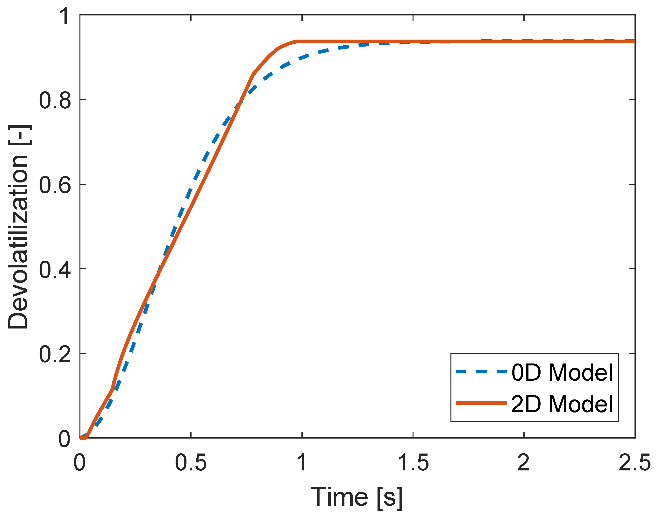
An example of a fitted curve and the semi-2D cylindrical model output can be seen in
Figure 2.
2.4. Chemometrics
Chemometrics is a statistical approach to extract data from chemical or biological data sets. A common method within chemometrics is partial least squares regression (PLS) [
31,
32]. In PLS, a correlation between a matrix of input variables (
X) and an output variable (
Y) is determined. PLS is a linear regression method. An in depth description of PLS is beyond the scope of this manuscript, but can be found elsewhere [
31,
32,
33,
34]. The PLS models presented here are calculated in PLS Toolbox version 8.1.1 and Matlab version 9.3.0 (R2017b).
2.4.1. Parameter Definition
The input parameters tested for the calculation of
A and
E in the 0D model are particle radius, particle density, gas temperature, and particle aspect ratio, as they have previously [
10,
24,
35] been shown to influence the devolatilization process. The applied parameter spans for each variable can be seen in
Table 2. They cover the parameter variations relevant for biomass suspension firing conditions. A total of 35 simulations with the semi-2D model have been made to span the parameter space. The applied parameter values for each simulation can be seen in the
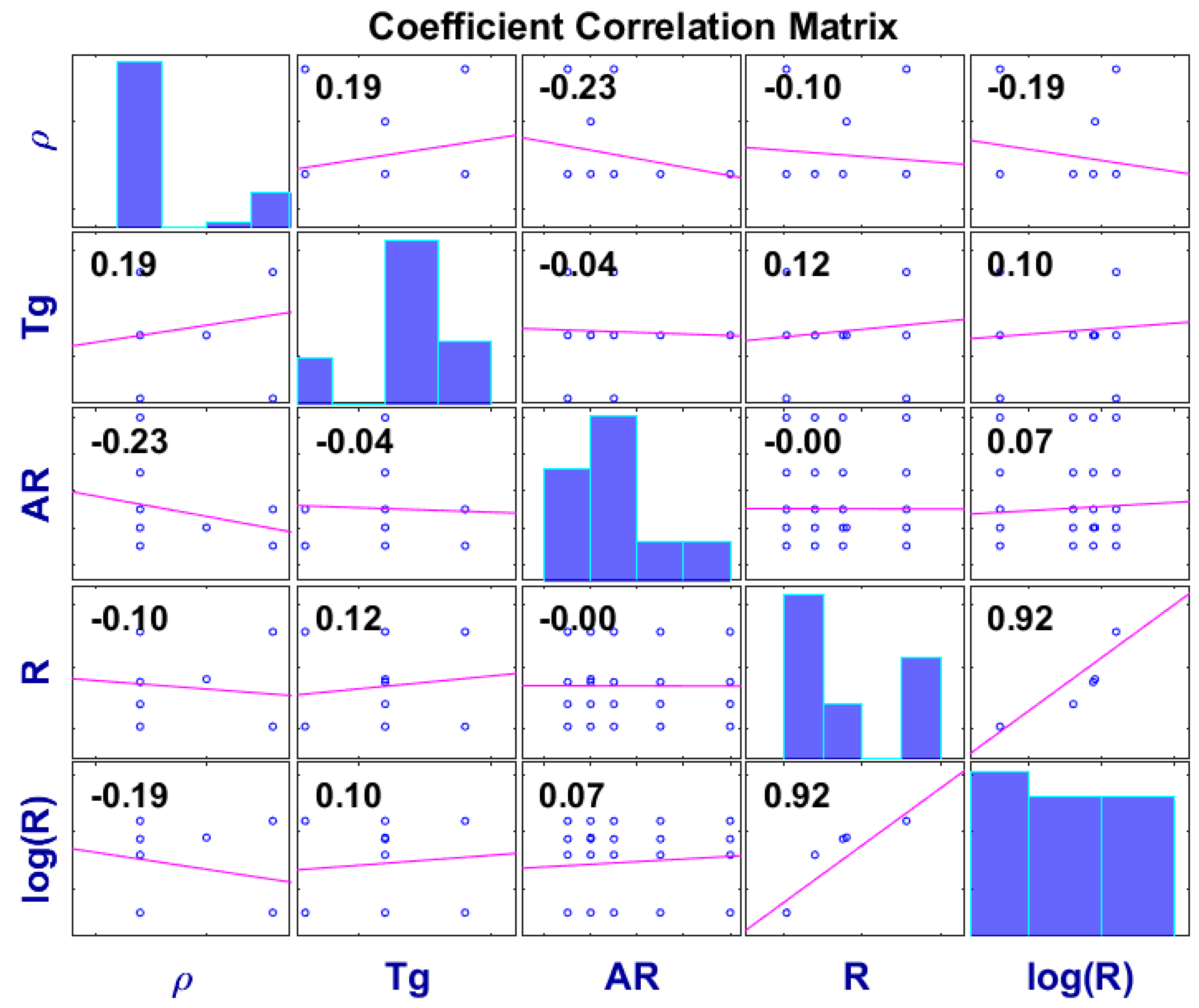
Appendix A. To show the correlation (negative or positive) between input parameters, the correlation coefficient chart is made. It is shown in
Figure 3. The higher the absolute value in the correlation coefficient matrix, the higher degree of correlation between two input parameters. When the degree of correlation is high, the effect of each input parameter cannot be separated due to confounding. Here the degree of correlation is numerically low (≤0.23), which means the influences on the model results can largely be ascribed to each individual input parameter.
2.4.2. Preprocessing
Preprocessing is an important step in PLS, and the individual preprocessing methods tested can be seen in
Table 3 and
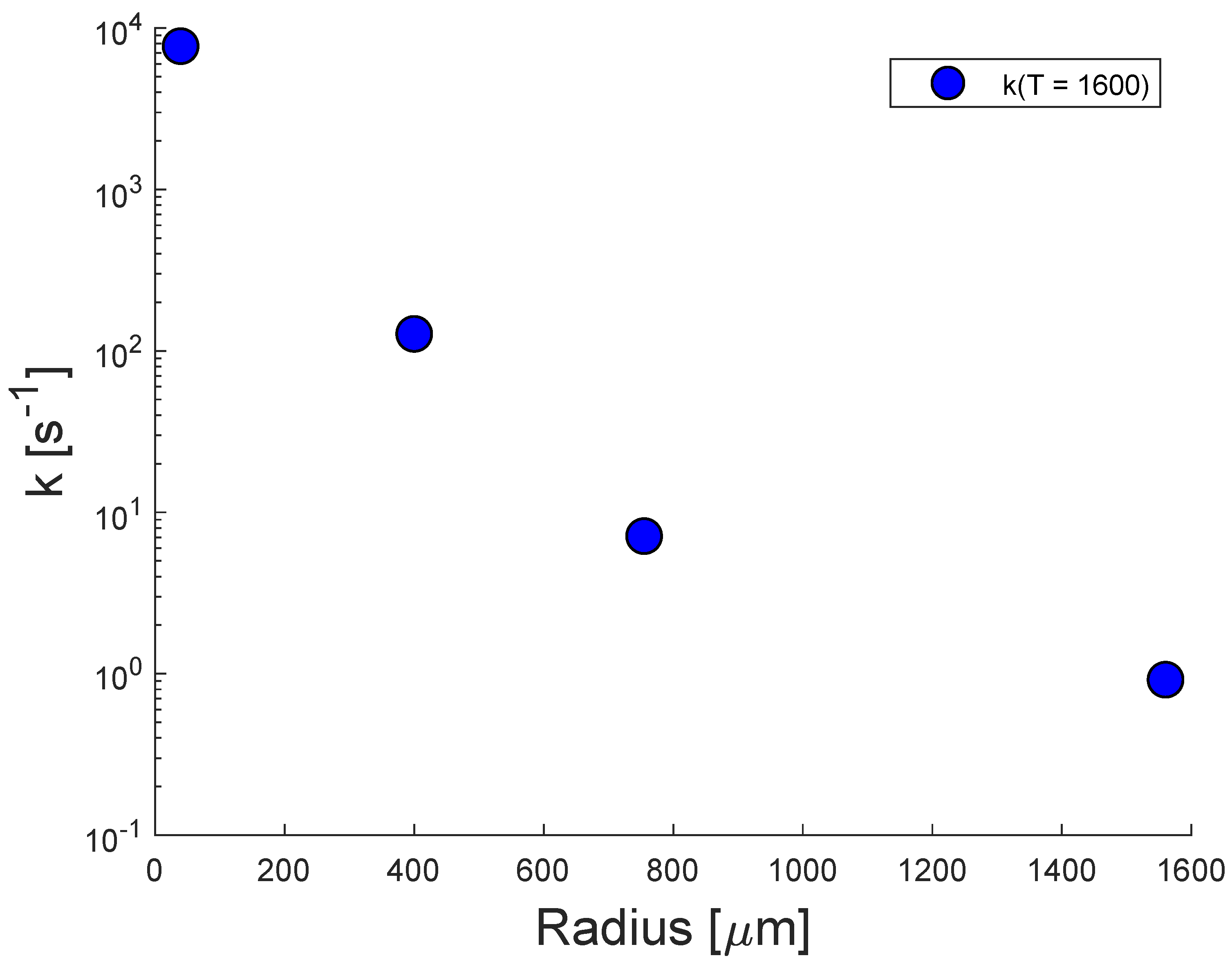
Table 4. When studying, e.g., the effect of the particle radius on the Arrhenius parameters, it is clear that the correlation is nonlinear as seen in
Figure 4. Thus, both
R,
,
, and
have been tested, and the quality of the preprocessing is then determined based on the explained variance for the input matrix (ExpVar(
X)), the output parameter (ExpVar(
Y)), and the root mean squared error of cross validation (RMSECV) for both
A and
E, respectively. Similar considerations have been made for determining the preprocessing of
,
, and
. In these cases, the nonlinearity of the correlations between input and output variables are so weakly pronounced that no significant improvement is added to the model by choosing various more complex preprocessing methods and thereby increase model complexity beyond what is necessary.
Furthermore, the input variables here are not on the same scale, so to account for this, all input parameters have also been scaled to account for unit variance.
2.4.3. Cross Validation
The cross validation is made to ensure that the presented model is robust. It can be done in many ways; here, the random subset method [
36] is used with 6 splits and 20 iterations, thus on average 17% of the data set is removed in each iteration. All models have been made with two PLS components. When doing the cross validation, preferably the obtained RMSECV values should be low, and ExpVar values high. The values in
Table 3 and
Table 4 are the basis for choosing the relevant preprocessings for a model. Due to the lower RMSECV(
A) and RMSECV(
E) and higher ExpVar(
X) (compared to the number of input data in
X) and ExpVar(
Y) values, model 2 has been chosen both for
A and
E. If models appear equally good or almost equally good based on RMSECV and ExpVar data, the simpler model is usually preferred within PLS.
5. Conclusions
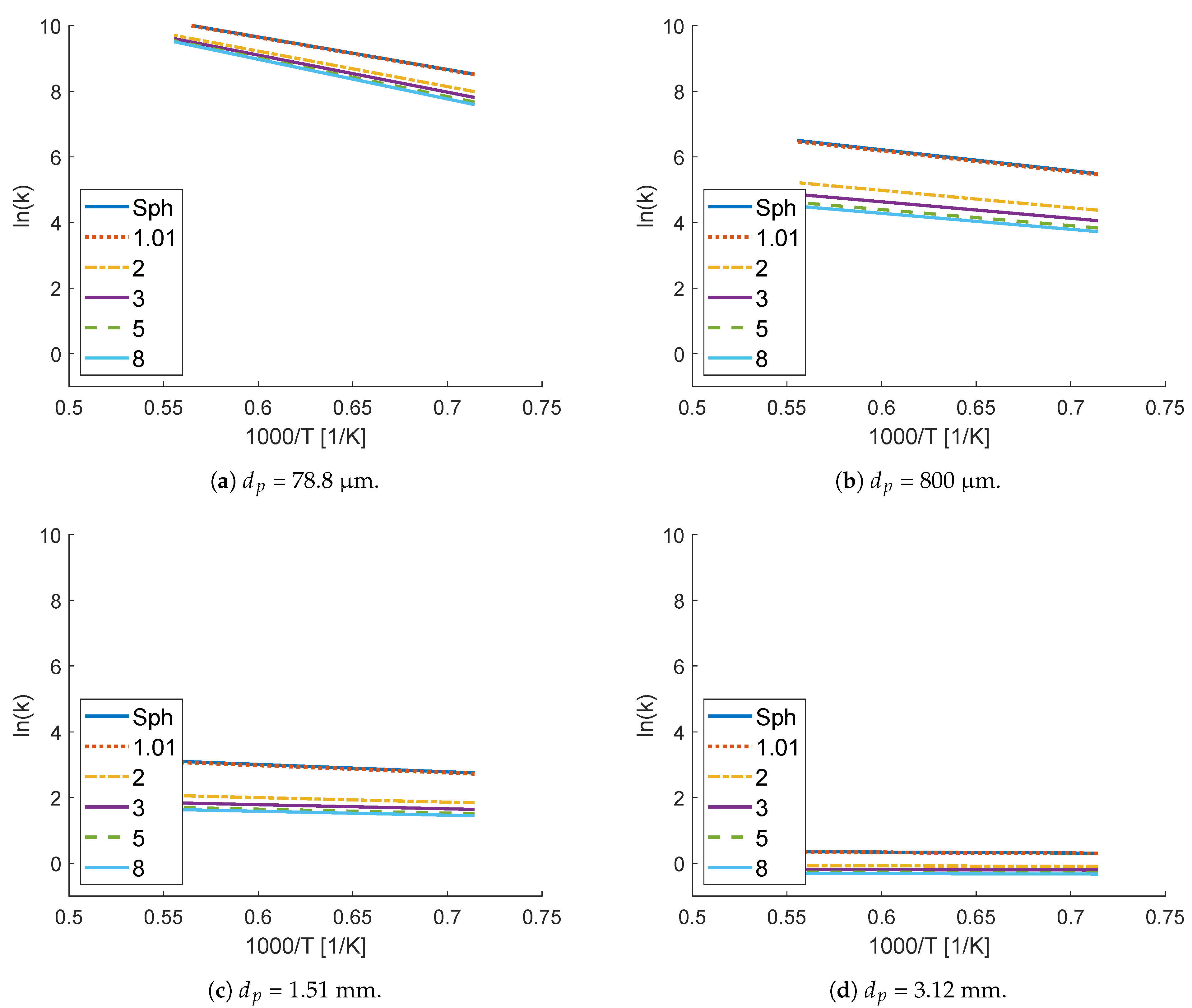
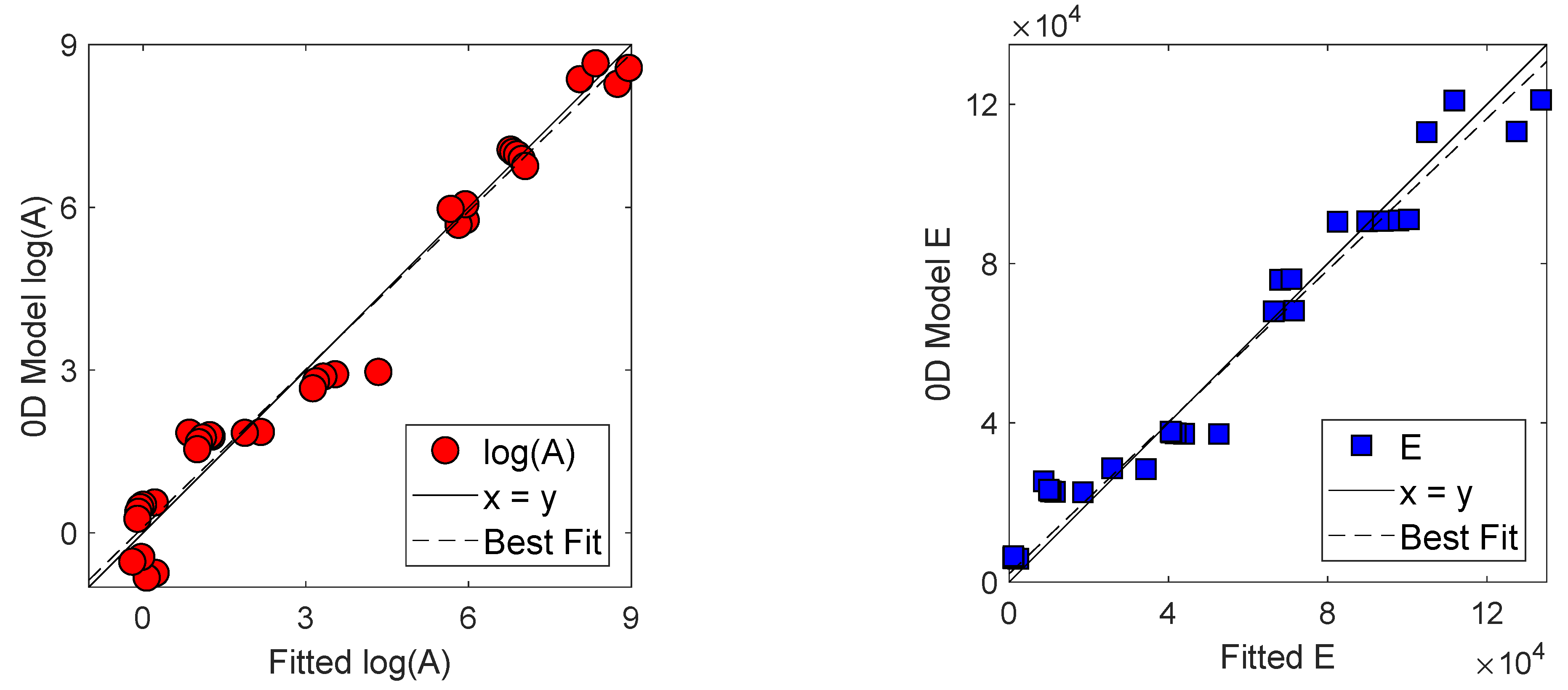
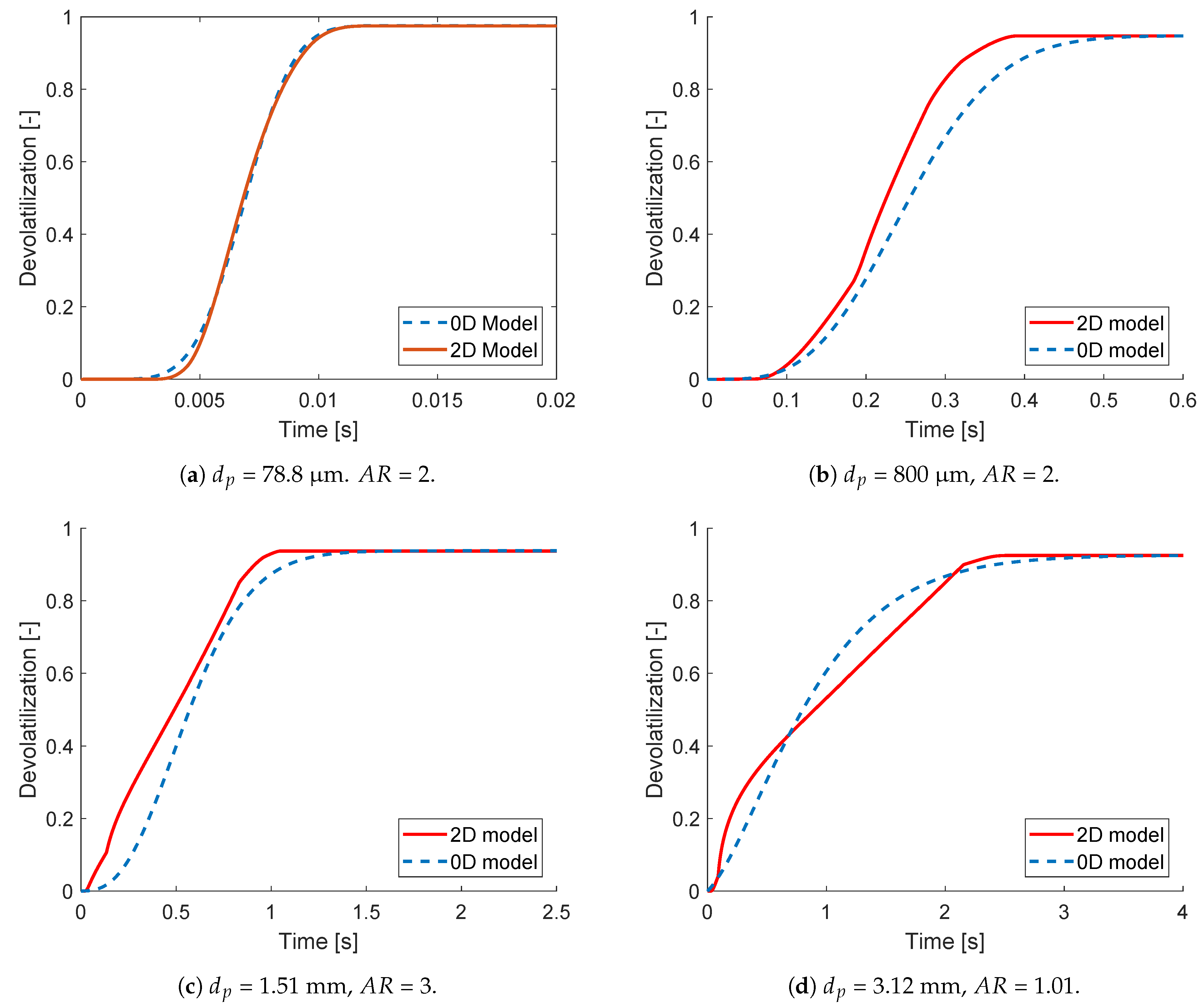
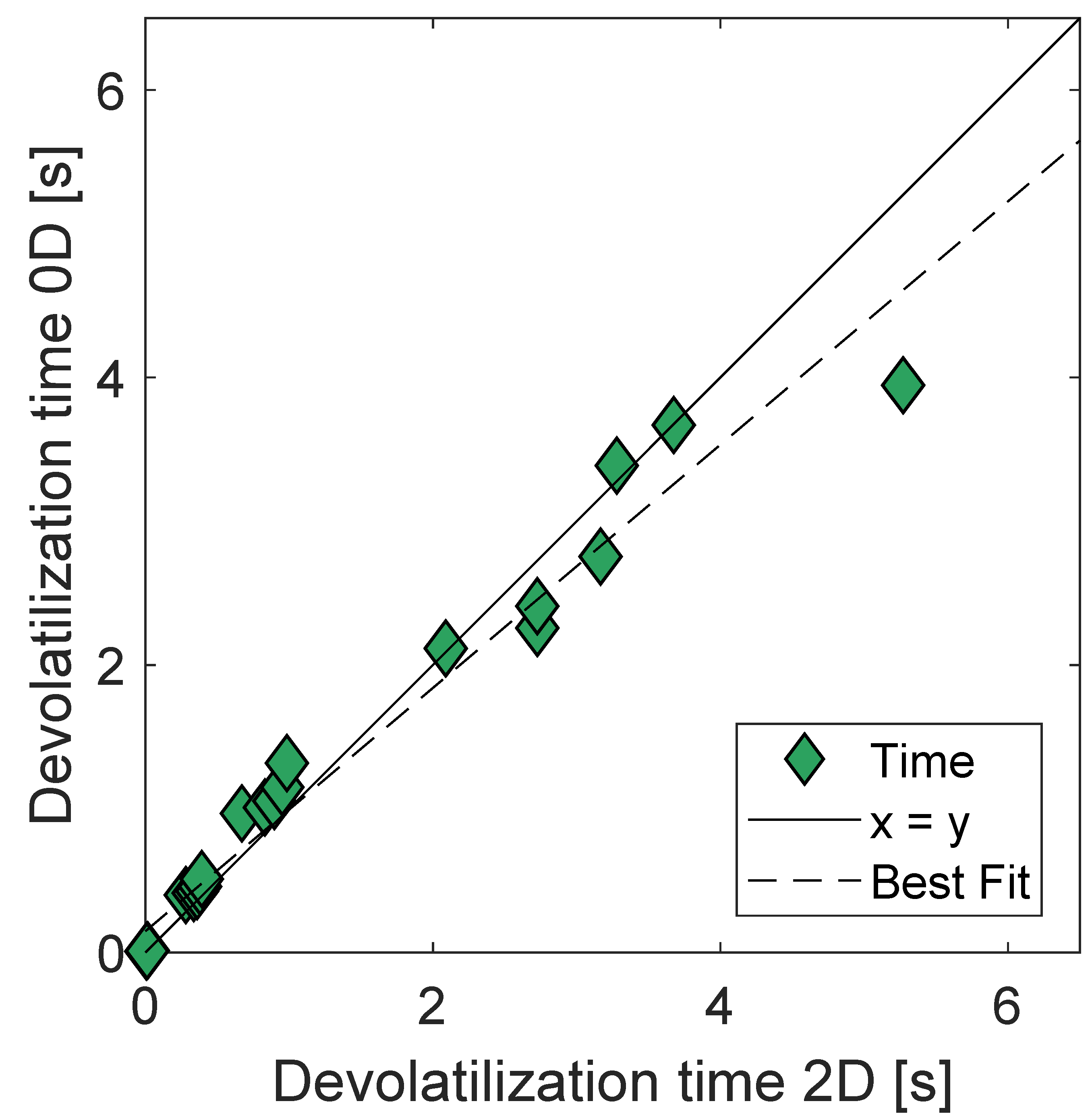
A 0D model has been developed to describe devolatilization of cylindrical biomass particles using a lumped single first order Arrhenius equation to account for both kinetics and heat transfer limitations in the particle. The model accounts for aspect ratio, particle density, gas temperature, and particle radius, because of their influence on devolatilization rate and on flame shape and stability. Including these parameters in the devolatilization model allows for better CFD simulations of industrial sized units. Calculations show that of these parameters, especially particle radius and temperature, are important for the prediction of the degree of particle devolatilization. Model predictions are compared to those of a more complicated semi-2D model, showing good agreement, especially for the smaller particles, where the heat transfer limitation is less severe. The presented model also shows that it is important to include differences in aspect ratio, but that the influence of aspect ratio on devolatilization rate levels off as aspect ratio increases and consequently end effects become less important.
The devolatilization model presented is simple and can be implemented into CFD without adding substantially to the computational costs. By implementation into CFD simulations, as, e.g., the ones described by Johansen et al. [
8], it is likely that an even greater match between numerical simulations and the physical phenomena during flame development in a suspension firing unit can be obtained. Future work should include making the CFD simulation described above, and expanding the model to include different kinds of biomass and municipal waste.


