Abstract
Heat demand of buildings and related CO2 emissions caused by energy supply contribute to global climate change. Spatial data-based heat planning enables municipalities to reorganize local heating sectors towards efficient use of regional renewable energy resources. Here, annual heat demand of residential buildings is modeled and mapped for a German federal state to provide regional basic data. Using a 3D building stock model and standard values of building-type-specific heat demand from a regional building typology in a Geographic Information Systems (GIS)-based bottom-up approach, a first base reference is modeled. Two spatial data sets with information on the construction period of residential buildings, aggregated on municipality sections and hectare grid cells, are used to show how census-based spatial data sets can enhance the approach. Partial results from all three models are validated against reported regional data on heat demand as well as against gas consumption of a municipality. All three models overestimate reported heat demand on regional levels by 16% to 19%, but underestimate demand by up to 8% on city levels. Using the hectare grid cells data set leads to best prediction accuracy values at municipality section level, showing the benefit of integrating this high detailed spatial data set on building age.
1. Introduction
It is widely agreed that global carbon dioxide (CO2) emissions need to reach net-zero around the year 2050 to mitigate global warming to below the internationally agreed upon threshold of 1.5 °C above pre-industrial levels. As part of this emission reduction process, a rapid, global transformation of the energy and building sectors will be necessary within the next few decades. This includes the prevailing use of renewable energy resources accompanied by a steep increase in energy efficiency to reduce energy demand in terms of electricity and heat [1].
Today 74% of Europe’s population live in cities and urbanized areas [2], which goes alongside an enormous demand for heating and the use of warm water at these places. Heat demand for buildings adds up to almost 80% of the total heat demand, which again makes up around 50% of the final energy demand in the member states of the European Union [3]. In addition to measures that reduce the overall heat demand, like refurbishment of old buildings, the use of more efficient heating systems is needed to substantially reduce energy related CO2 emissions. With the expected future increase in air temperatures due to climate change, heat demand may decrease in winter seasons, but energy demand for cooling of buildings in summer may grow [4].
In 2018, only round 21% of the EU-27′s total energy demand for heating and cooling was covered based on renewable resources [5]. District heating can offer a solution to increase the share of renewable energy in the heating sector, especially in densely built-up and inhabited areas like cities. It provides the ability to integrate different locally available renewable heat resources like deep geothermal and solar thermal energy or industrial excess heat as well as often necessary seasonal heat storages into renewable energy systems [6,7].
To support heat planning at various scales in general and to establish new local heating networks, preferentially operating with heat from renewable resources, reliable data on heat demand for a given area is essential [8,9,10,11,12,13,14]. Areas probably suited for district heating can be detected based on information on heat demand density [15]. Since measured data on heat consumption are usually not publicly available, various mapping approaches have been developed, helping to quantify heat demand of buildings and to localize the potentials for district heating. These approaches are often based on Geographic Information Systems (GIS) and range from the scale of a district [16,17], a municipality or a city [18,19] up to national [15,20,21,22,23], continental [24,25] and even global levels [26].
However, heat demand modelling and mapping is highly limited by the availability and quality of input data sets. In many cases, 3D building stock models are used as base data for heat demand mapping. They provide the geometrical information of individual buildings and information about the building’s use for the building stock of a district, city or state [27,28,29,30]. Nowadays, 3D building stock models are available in several European countries [19,31,32,33]. Usually, semantic information (e.g., construction year or period, number of floors or floor heights, refurbishment status), which is known to be crucial for calculating heat demand [30,34,35,36,37] is missing. This information needs to be added to a building stock database [29,38].
Data on the building age are essential here [34], since most heat demand modelling approaches use building archetypes from building typologies to quantify heat demand. Building typologies are often derived from statistical records based on regional or national building stock registers or from detailed models of single buildings of a certain type and age [38,39,40,41]. They provide information on average heat consumption per unit area for each building archetype of a certain construction period.
Detailed building stock registers, stating each building’s year of construction are only available for a limited number of countries [7,41,42]. In other cases, the required data need to be laboriously collected by on-site mapping or from local building cadasters [28,29], commercial data sets [17,37], from remote sensing data [43] or directly from house owners and occupants [44]. In this paper we present an alternative approach using readily available census data in order to optimize the prediction of building-related heat demand from regional to sub-regional scales.
Recently, results of the European Union population and housing census 2011 [45], that include data on building stock age, are made available by EU and national authorities in high spatial resolution [46,47]. This census has been conducted in all EU member states and its data comprise different levels of aggregation, ranging from state to address level. These data are suited to support heat demand mapping at the various spatial scales [24,34,38,48,49,50,51].
To our knowledge, the question to what extent the integration of this census data on different spatial aggregation levels contributes to improvements in heat demand mapping, i.e., to minimizing the estimation error, is unresolved.
Based on a regional 3D building stock model of a German federal state, supplemented by regional information on building age from the census of 2011 aggregated on two different spatial levels, we test the prediction quality of modeled heat demand against reported heat demand and measured gas consumption data.
In more detail, the objectives of this study are (I) to present a GIS-based bottom-up approach, operating on available, official regional geo and census data, used for modelling and mapping building heat demand at the regional and sub-regional scales, (II) to quantify the estimation error of calculated heat demand by comparing differently composed sets of census data against a reference and measured data, and (III) to demonstrate the practical use of the outlined, improved heat demand mapping approach for heat planning.
2. Materials and Methods
2.1. Study Region
The north German federal state of Schleswig-Holstein (Figure 1) produced 23 TWh of electricity from renewable resources in 2018. This exceeded its total electric power demand by 53% and therefore positions the state as a forerunner in the German energy system transition in terms of electricity. Nevertheless, in the heating sector, the federal state so far covers just 14% of its total heat demand from renewables, just like the whole of Germany. Heat demand (40 TWh) dominates the overall energy demand of the federal state, if compared to the electricity (15 TWh) and traffic sectors (22 TWh). The biggest share of the annual heat demand (78%) is caused by residential and commercial buildings with their demand for space heating and hot water provision [52].
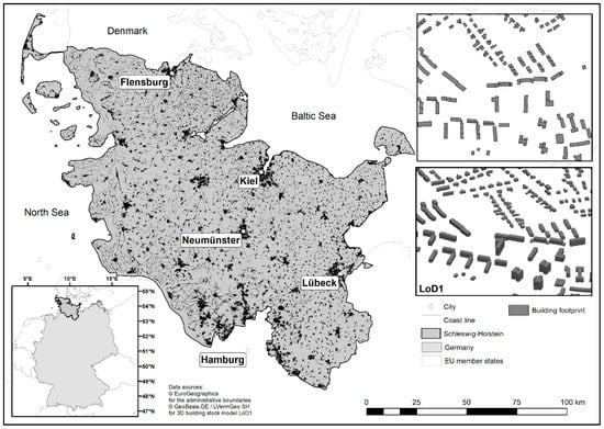
Figure 1.
3D building stock model for the German federal state of Schleswig-Holstein and major cities.
The share of district heating in the federal state was at 11% at the time of the European census in 2011. In the capital, the City of Kiel, already 30% of residential buildings were connected to an existing district heating system, and this was even 91% in the City of Flensburg. In most other cities and municipalities, the heating sector is dominated by gas and oil-fired central heating [47].
A well informed, structured heat planning process could help to identify areas with further district heating potential (as well as nearby renewable heat resources) in order to increase the share of renewable heating to more than 22% already in 2025 as stated in the climate protection act of the federal state [52].
Unlike in the electricity sector, cities and municipalities have to plan and organize the transformation of the local heating sector on their own. Therefore, the climate protection act of the federal state enables them to do structured heat planning for their territory. Recently, a first geo data set, giving municipalities an overview on the spatial distribution of regional heat demand, has been available for the federal state [53], but it is based on a top-down method using regionalized input data of European scale [24].
2.2. Input Data
2.2.1. 3D Building Stock Model
For this study, a regional 3D building stock model for the whole area of the study region was provided by the federal state’s surveying authority [54]. About 1.8 million building models (Figure 1) represent the regional building stock as modeled by the surveying agency at the end of the year 2017.
All buildings are modeled in a “level of detail 1” (LoD1), meaning surveyed building footprints are extruded by the building height (Figure 1). Building height was measured by the surveying authority via airplane by light detection and ranging (LiDAR) with a height accuracy of +/−5.0 m. Heights in the models represent the averaged roof top heights detected.
For most of these building models, information on the type of usage is available. All buildings without any information on usage (14%) were excluded from further processing. A random sampling by the authors showed that these building models mostly represent small unheated garages or sheds. Moreover, all building models with a non-residential usage (42%, including mixed used buildings) were disregarded in this study, since information on building age from the census was only available for pure residential buildings, as described in the following. In total 808.485 residential building models remained and were used in the heat demand modelling approach.
2.2.2. Spatial Census Data Sets on Construction Period
Two different spatial data sets on building age were used in this study: a regional cadaster, as well as a national data set, both containing aggregated results of the census from 2011 (Figure 2).
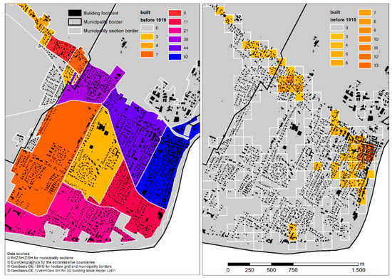
Figure 2.
Census information on construction period aggregated on municipality sections (left) and on hectare grid cells (right) showing the number of residential buildings built before 1919 in this area.
In the regional cadaster [55], the original address-based census results were aggregated by the regional statistics authority in 10 construction period classes for about 13,000 municipality sections representing most municipalities in the study area (Figure 2 left). Unfortunately, the cadaster did not cover the four major cities of the federal state (Kiel, Lübeck, Flensburg, Neumünster), since they have independent local departments for statistics, who did not participate in the cadaster project. Nevertheless, for this study it was possible to use the spatial information on the construction period for residential buildings for all other municipalities. Due to protection of data privacy, original information for some age classes in some municipality sections had been changed by the regional statistics authority via an algorithm. This was to ensure that a minimum of 3 residential buildings with the same construction period class were present or no information for this class is reported. In total, 9397 municipality sections contained information on the number of residential buildings per construction period.
A second spatial data set with aggregated results of the census was published by the statistical offices of the German federal states [47]. It contains a grid identifier that allowed the joining of the information to an existing, nationwide spatial grid. This grid has a spatial resolution of one hectare and is provided by the national surveying authority. For this study, all grid cells representing the study region Schleswig-Holstein (including the area of the four major cities) were selected from the national grid and joined with the regional census results in a spatial database. Each hectare grid cell then reports the number of residential buildings in this specific area for each of 10 predefined classes on the construction period (Figure 2 right). Again, some aggregated data had been changed in a privacy protecting way by the regional statistics authority. In total 84,876 cells contained information on the construction period for residential buildings.
2.3. Heat Demand Modelling Approach
2.3.1. Data Processing
Preparation and processing of input data, modelling of heat demand and final mapping of results was performed using two different combinations of Geographic Information Systems (GIS) (ArcMap, QGIS), geodatabases (file geodatabase, PostgreSQL database with spatial extension PostGIS) and programming languages for scripting (Python, R) in parallel, in order to test and show simple reproducibility and transferability of the applied method.
2.3.2. Modelling of Heat Demand Density
Annual heat demand of residential buildings was modeled according to the German building energy saving ordinance [56]. In a first step, the number of floors (NF) had to be derived from the building height (bh) according to (1), assuming a floor height (fh) of 3.50 m:
NF = bh [m]/fh [m]
According to [56] the heated floor area of a residential building should be calculated based on the combined volume of all heated building parts. In this study, the heated building volume (HBV) is simply based on the overall cubic content of the building model. It is calculated according to (2) by multiplying the ground floor area (gfa) with the building height:
HBV = gfa [m2] × bh [m]
Due to the comparatively large assumed floor height of 3.50 m, a special formula (3) from [56] was used to calculate the heated area (HA) of buildings based on the HBV:
HA = (1/fh [m] − 0.04 [m−1]) × hbv [m3]
According to [57], residential buildings with a total HA below 55 m2 can be regarded as unheated in Germany. Therefore, these building models were excluded from the further processing steps and 770,252 heated residential buildings remained for heat demand modelling. They were further subdivided into single-family houses (SFH) and multi-family houses (MFH). Following again [57], all heated residential buildings with a ground floor area of more than 250 m2 or more than 2.5 floors can be regarded as MFH in Germany as well as in the study region. This resulted in 689,282 SFH and 80,970 MFH, which were combined with information on the construction period from the two spatial census data sets (Figure 3).
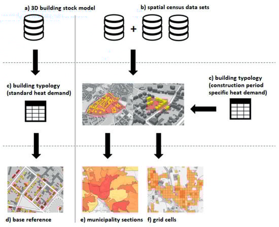
Figure 3.
Data processing and method flow schema: the provided 3D building stock model (a) and two available spatial census data sets (b) were combined with building type or construction period specific standard heat demand values from a regional building typology (c) to create a base reference data set (d) and two enhanced data sets (e,f) on the heat demand of residential buildings.
A base reference model was created first, in order to later evaluate the usefulness of the two different spatial census data sets to improve heat demand mapping (Figure 3a,c,d). For the base reference, the annual heat demand (HD) of all heated residential buildings was calculated according to (4), using just two building-type specific standard heat demand (SHD) values for SFH (171.3 kWh/m2) and MFH (150.5 kWh/m2):
HD = HA [m2] × SHD [kWh/m2 × a−1]
These two SHD values were taken from a building typology for the study region [58]. This regional building typology further provides more differentiated heat demand values for SFH and MFH archetypes from different construction periods (Table 1). Therefore, the summed-up information on the heated area per construction period from the two different census data sets was used with these construction period specific SHD values to calculate the annual HD for the municipality sections and the hectare grid data again for two improved models (Figure 3e,f).

Table 1.
Construction period classes used in the two spatial census data sets against classes of the regional building typology as well as corresponding standard heat demand (SHD) values for single- and multi-family houses (SFH and MFH) and values used in the presented method.
From the two spatial census data sets, municipality section and hectare grid cell IDs were assigned to all remaining heated residential buildings; if they spatially intersected (Figure 3c), the first intersecting ID was joined to each building in the building stock database. This was possible for most (86%) of the remaining residential building models; nevertheless, some building footprints are located outside municipality sections and hectare grid cells (e.g., residential buildings built after the census was conducted in 2011). These buildings were left without information on the construction period.
Summary statistics for each municipality section and grid cell were created, stating the summed-up HA for all SFH and MFH in this specific area. Additional information on the number of residential buildings per construction period were also joined to the two spatial data sets. Based on this second information, the share of buildings of a certain construction period in each municipality section and hectare grid cell was calculated and transferred to the HA of SFH and MFH in this area. This allowed the calculation of the residential building heat demand in each municipality section and grid cell by multiplying the share of summed-up HA per construction period class of SFH and MFH with annual heat demand values from the regional building typology (Figure 3c), as described in the following.
If information on the number of residential buildings from certain periods of construction was available in a municipality section or a hectare grid cell, the share of a certain period at the overall summed up HA in this area was multiplied with the SHD value of the corresponding SFH or MFH building archetype in the typology (Table 1).
Not all construction period classes, predefined in the census data sets by the statistics authority, fit to the classes of the building typology (Table 1). For the census construction period class “1949 to 1978” a mean value from SHD values of three classes of the building typology was used. If no information on the construction period was available, the heated area of SFH and MFH in this municipality section or grid cell was multiplied with the respective SHD values (171.3 or 150.5 kWh/m2) as already done in the base reference model.
In order to provide basic information for heat planning, the modeled annual HD per municipality section was further divided by the municipality section’s total area in order to state the heat demand density (HDD) in the same way as for the hectare grid cell results. An HDD of more than 150 MWh/(ha×a) indicates possible areas suited for district heating in the study region [24,53,59].
In summary, the two available census data sets were used to assign more appropriate standard heat demand values to the summed-up heated area per construction period class in each municipality section and hectare grid cell to create two improved spatial data sets on annual heat demand density for the study region.
2.3.3. Validation of Results
Official statistical data on residential building heat demand for the whole federal state, for two cities and for a county in the study region were available from authorities and local energy concepts. They were used for a first rough validation of the modeled heat demand on regional and sub-regional scale.
For a more detailed validation on a sub-regional level, measured gas consumption for about 25,000 individual gas meters, located in residential buildings of a city in the study region, were provided by a local utility company [60]. After joining the originally address-based locations of the meters to the corresponding residential building models, excluding outliers (cut-off 0.05) and adjusting the measured data to the long-term average weather and climate conditions in the region via postal code zones, finally 11,626 gas consumption values remained for validation.
In order to state and compare the goodness of fit for the three models (base reference without any information on the construction period, methods enhanced with the municipality sections data set and with the hectare grid data set), pairs of measured and modeled heat demand for individual residential buildings were aggregated on municipality level. The fit was then described by calculating the statistical measures Mean Absolute Percentage Error (MAPE), Root Mean Squared Error (RMSE), and the coefficient of determination (R2) using the software environment “R” [61].
3. Results: Heat Demand Mapping at Regional and Sub-Regional Scales
3.1. Base Reference Model
Figure 4 shows the resulting spatial distribution of annual residential building heat demand in the study region for the base reference model. Modelled heat demand is mapped on the two different spatial aggregation levels used in this study. In total, an annual heat demand of 25,783,181 MWh was modelled for the whole study area, when using no information on the construction period.
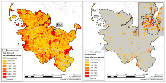
Figure 4.
Heat demand of residential buildings modeled without information on construction period mapped on municipality sections (left) and hectare grid cells (right) for the study region Schleswig-Holstein and the municipality area of the City of Kiel.
In 89% of the 12,876 municipality sections of the federal state (Figure 4 left), heated residential buildings were located and the annual heat demand could be modeled. On average, 1850 MWh per year are demanded by a municipality section. The maximum heat demand per section reached 112,106 MWh while the minimum was at 10 MWh per year. As mentioned above, for the four major cities no census data and therefore also no municipality section geometries were available in the provided cadaster data. Therefore, results were aggregated on the total municipality area for these cities. For the capital, the City of Kiel, a total residential building heat demand of 1,682,738 MWh per year was modeled (Table 2).
Table 2.
Annual residential building heat demand per city and county in the study region for the base reference model without any information on building age and for the two models enhanced by spatial data sets on the construction period of residential buildings.
Mapping the base reference model on hectare grid level (Figure 4 right), the total heat demand is located in only about 10% of the 1.6 Mio. ha representing the study region, due to the spatial concentration of the heated (multi-family) residential building stock in urban areas like in the City of Kiel. On average, annual heat demand is 164 MWh per hectare, but with a standard deviation of 186 MWh. The highest heat demand per hectare (5134 MWh) is located in a densely built-up residential area, while the lowest value of 9 MWh represents a single residential building in a grid cell. In just about 4% of all 1.6 Mio hectare grid cells representing the study region, the threshold value for demand density of 150 MWh per year, indicating a possible suitability for a district heating network, is exceeded. For the City of Kiel this is the case for 25% of the 11,852 hectares representing the city, summing up to 1,620,328 MWh (96%) of the city’s annual heat demand in the base reference model.
3.2. Comparison of Base Reference Model against Model Using Municipality Sections Data Set
Integrating the municipality sections data set with spatial information on the construction period of residential buildings into the modelling process resulted in a total annual residential building heat demand of 25,417,136 MWh for the whole study region. This is a decrease of 1.4% compared to the base reference model result described above. Nevertheless, this reduction of 366,045 MWh is around a third to a half of the residential heat demand of an average city in the study region.
Comparing these enhanced results with the base reference model on city and county levels (Table 2) shows that, in the four major cities (including the City of Kiel), no changes in the results can be observed when using the municipality sections data set, due to the missing spatial information on the construction period in these areas. For the remaining 11 counties of the study region, just minor differences in the aggregated modelled annual heat demand occur.
When comparing this first enhanced model with the base reference model results in more spatial detail for the 11,423 municipality sections (without the 4 major cities), the mean annual heat demand slightly decreased by 1.7% to 1818 MWh while the maximum value increased by 3.6% to 116,112 MWh. The minimum residential building heat demand stayed more or less the same with about 10 MWh. Nevertheless, for individual municipality sections, changes in the range of +15% to −49% with a maximum increase of 4015 MWh and a maximum decrease of 7418 MWh occur (Figure 5 left), when enhancing the heat demand modelling process by including the municipality sections data set with information on the construction period.
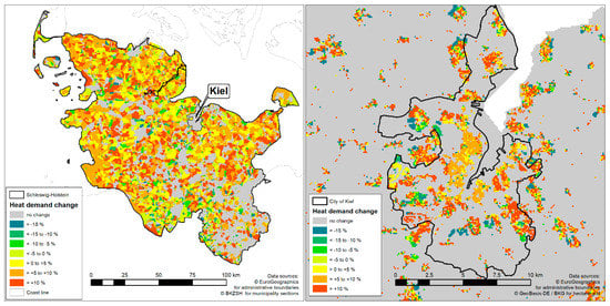
Figure 5.
Percental change in annual residential heat demand when modeled with information on residential building construction period on municipality sections (left) and hectare grid cells (right) in comparison to the base reference model without any information on building age.
3.3. Comparison of Base Reference Model Against Model Using Hectare Grid Cells Data Set
Integrating the hectare grid cells data set with information on the construction period of residential buildings into the modelling method, resulted in a total annual residential building heat demand of 25,968,973 MWh for the whole study area. This is a 0.7% (185,792 MWh) increase when compared to the base reference model result, where no information on the construction period was used. Compared to the results of the model enhanced with the municipality sections data set presented above, this is a 2.1% (551,837 MWh) increase in modeled total heat demand.
Comparing the results on city and county level with the municipality sections data set results (Table 2), shows an increase in modeled heat demand for the four major cities in the study area, since now detailed spatial data on the construction period were available for the areas of these cities. This led to more spatially differentiated results based on the local periods of construction, emphasizing the often above-average old building stock with a high share of big multi-family houses in the city centers and old-towns. Their high heat demand is not compensated or leveled by the lower heat demand modeled at the outskirts of the cities, representing often new single-family residential buildings in new developed housing areas with a lower heat demand (Figure 5 right).
The modeled residential building heat demand for the City of Kiel therefore increased by 4% to 1,752,221 MWh compared to the results of the method enhanced by the municipality sections data set and the base reference results. Looking at the county level also reveals an increased heat demand for all 11 counties in the range of 1% to 3%, when compared to the results of the method enhanced by the municipality sections data set (Table 2).
The mean modeled heat demand per hectare grid cell is now at 165 MWh per year, compared to 164 MWh in the base reference results, but with an increased standard deviation of 192 MWh. The highest annual demand per hectare decreased to 4967 MWh, while the lowest heat demand per hectare decreased to just 5 MWh, when compared to the hectare grid results of the base reference. In individual hectare grid cells, the changes in modeled heat demand, compared to the reference results, range from −51% to +15% (Figure 5 right).
Heat demand density exceeds the threshold value of 150 MWh/(ha×a) now in just 60,962 grid cells, compared to 61,574 in the base reference results. This represents a decrease of 612 ha in the potentially suited area for district heating. Within the City of Kiel, 2890 hectares with a district heating potential are located (24% of the city area) that sum up to 1,657,030 MWh annual heat demand which is a share of 95% of the total residential building demand modeled for the city.
3.4. Validation of Results
In Table 3 available official statistical data from 2018 on total annual heat demand for space heating and hot water in residential buildings for the whole federal state [52] are compared to the results of all three heat demand models described above.
Table 3.
Comparison of reported and modelled residential heat demand on different spatial levels.
In general, all three models overestimate the reported heat demand on these regional aggregation levels by 16% to 19%. The model improved with spatial information on the construction periods from the municipality sections data set shows the lowest overestimation on the federal state level. Using the hectare grid data set with information on the construction period results in an even higher overestimation of the reported numbers than in the base reference model on this regional level.
For the county of Dithmarschen, residential heat demand estimated and reported in an energy concept [62] is also overestimated by all three approaches, but to the smallest extent in the base reference model without spatial information on residential building construction periods.
Nevertheless, on sub-regional levels, compared to reported annual residential heat demand from a climate protection masterplan for the City of Kiel [63] and compared to reported data for heat consumption from the district heating network of the City of Flensburg [64], the model enhanced by the hectare grid data set very well represents the reported heat demand for 2014 and 2016, respectively, while the base model and the model enhanced with municipality sections data show higher deviation, underestimating reported demand.
Using metered gas consumption from a city in the study region for validation purposes, also reveals an underestimation of measured heat consumption. Absolute heat and gas consumption values are not shown here due to data privacy reasons. Demands modeled in the base reference deviate with +/−8% to 24% from measured consumption, depending on the municipality section. When using information on the construction period from the municipality sections data set, these absolute deviations change to a range of +/−10% to 23%. Using the hectare grid data set, the range of absolute deviation goes down to +/−8% to 22%. All three approaches show a tendency to underestimate the real metered heat consumption in this example city.
In general, lower MAPE and RMSE as well as a higher R2 are calculated for most of the 17 municipality sections of this city when enhancing the modelling and mapping approach with spatial information on the construction period (Table 4). Results from the model enhanced with the hectare grid cells data set show lowest MAPE and RMSE as well as a highest R2 values in most sections.
Table 4.
Statistical measures stating prediction accuracy on the municipality section level when validating modeled residential building heat demand with gas consumption data via address-based pairs.
4. Discussion
4.1. Heat Demand Mapping at Regional and Sub-Regional Scales
Compared to results of other studies, percental deviations in the above-mentioned ranges between reported, respectively, measured and modeled heat demand seem reasonable when using a 3D building stock model with a level of detail (LoD) 1, enriched with spatial information on the year of construction or construction period of buildings for residential heat demand modelling.
For example [16] also used LoD 1 models of buildings in a district in the City of Rotterdam combined with available information on the year of construction for each building. They overestimated the total heat demand of the district by 25% and reported a MAPE of 49% on zip code level, compared to the measured gas consumption of the same district.
As [34] and also [36] showed, these deviations decrease when using more detailed geometric and semantic input data as for example a LoD2 building stock model enriched, besides the year of construction, with information like renovation dates or the actual counted numbers of floors. A method developed by [65], based on LoD 2 building stock data enriched with information on the number of floors and the construction period from a local cadaster was used by [66] to model heat demand of an area in a district of Berlin, stating an average percental deviation of 19%.
The influence of using a more complex geometric input data set in combination with rich semantic data was again shown by [67] when comparing modeled heat demand per building block to recorded gas consumptions of two districts in German cities. First a LoD 1 building stock model was used in combination with detailed semantic information on the year of construction, on refurbishment dates, window-to-wall ratios and basements for each building. Second a LoD 2 building stock model was used. Reported mean deviation for the total heat demand in the study area when using the LoD 1 was 21%. On building block level overestimation of heat demand in the range of +5% to +30% were reported with the LoD 1. When using the LoD 2 building stock model and comparable semantic data in another study area, mean deviation of the total heat demand was reduced to 7% compared to gas consumption data, while on individual building level deviations of −18% to +32% were observed.
Looking at studies applying statistical methods instead of building archetype approaches, [68] used building parameters available from an LoD 2 building stock model of the canton of Geneva in Switzerland combined with information taken from the Geneva building cadaster including address-based information on the number of floors and year of construction in several regression analyses for different building types. For residential buildings they reached an MAPE of 17.8%.
Instead of a 3D building stock model, [22] used a Danish building cadaster with detailed, address-based information on age class and other semantic data for all buildings in the country as well as reported energy consumption for around 300,000 buildings. They combined it with a building typology to model heat demand of all buildings in the country and reached deviations of 1% to 15% per building compared to recorded gas and district heating consumption, while higher deviations were found for non-residential buildings.
Applying a building parameter-based statistical modelling approach to downscale zip-code aggregated gas demand to single buildings with a multiple linear regression analysis for the city of Rotterdam, the authors of [69] were able to reached a MAPE of 13% with an absolute deviation of the total average heat demand per building of just 2%.
In a review article on Urban Building Energy Modelling (UBEM) which includes, in contrast to heat demand mapping, beside building geometry data and building archetypes, also information on used materials, construction standards, local climate and weather, and usage patterns of dwellers. The authors of [70] name typical deviations to measured heat demand in the range of 7% to 21% for annual heat loads and 1% to 19% when looking at results for specific heat demand values.
4.2. Limitations of the Presented Approach
Modelling of building geometry in the LoD1 building stock model is based on averaged heights derived from laser scanning data or by photogrammetry with a height accuracy of +/−5 m. Since in the heat demand modelling approach, the number of floors is derived from the individual building’s height, this can lead to an over- or underestimation of the real number of floors, influencing the assigned building type (single family or multi-family house), the applied specific heat demand value as well as the heated area. For some building models no information on the usage was provided which leads to an exclusion from heat demand modelling and, consequently, to an underestimation of total heated area in the study region. The assumption of a uniform floor height of 3.50 m brings further inaccuracy into the modelling process since this height is different for certain types of building and periods of constructions in reality. Consequently, the applied formula (3) from [56] may not always fit. Furthermore, no information on basements, of which some may be heated in the study region, was provided in the 3D building stock model.
The two spatial data sets with information on the construction period of residential buildings are based on a census from 2011, while the 3D building stock model represents the state of 2017; therefore, residential buildings and their heated area built after 2011 will not be attributed with an age-dependent specific heat demand value but just with a standard value. This leads to an overestimation of the heat demand in residential areas developed in the study area after 2011.
The census itself is based on a questionnaire filled in by house owners which brings in uncertainty into the data sets from the beginning. Due to German data privacy law, the originally address-based census data were aggregated on area units representing at least three buildings with the same attributes. Otherwise, the data were excluded or changed in a privacy-protecting way. This brings in uncertainty, especially in rural communities with low numbers of residential buildings per unit area.
Further inaccuracy is added by the age-dependent specific heat demand values derived from the regional building typology which are based on averaged heat consumption values measured from 2007 to 2009 [58]. Since in the meantime each year roughly 1% of the residential building stock was refurbished, the used specific heat demand values will not be representative for some parts of the residential building stock in some areas of the study area anymore. Relating the specific heat demand values to the total heated area based on the percental share of the periods of construction, again based on the count of buildings from a certain period, increases the inaccuracy in the modeled heat demand for some areas, especially if a mixture of residential buildings from different periods of construction is present in the area.
Other aspects influencing the annual heat demand of residential buildings, like vacancy and the different individual user behaviors, leading to different patterns of space heating and hot water usage in the same type of residential building, could not be considered in this study due to missing spatial information and data sets on these topics.
Regarding the mapped heat demand density, demand of non-residential buildings was not modeled and mapped in this study. Therefore, a part of the total heat demand is missing and mapped heat demand densities above 150 MWh/(ha*a) just show suitability for district heating when connecting residential buildings. Adding further heat demand of non-residential buildings like offices, stores and mixed used buildings would increase the number of areas potentially suitable for district heating.
5. Conclusions and Outlook
This study showed how different available spatial data sets with information on the construction period of residential buildings from the European census of 2011 can improve a 3D building stock model and a GIS-based bottom-up approach to model and map regional and sub-regional heat demand of the residential building stock at the example of a German federal-state.
Compared with official heat demand data on a regional level, modeled heat demand generally tends to overestimate reported demands and this even increases, when using spatial data sets on the construction period in the modelling process, especially when using the hectare grid cells data set.
Nevertheless, when validating the results on city and municipality section level, results tend to better agree with reported data and measured gas consumption and model fit parameters improve, again especially when using the hectare grid cells data set.
In conclusion, the data set aggregating census information on construction periods on a hectare grid turned out to be better suited than the municipality sections data set to improving the presented heat demand modelling approach in terms of accuracy on sub-regional level. It better represents the small-scale spatial variations in the age structure which allows a better allocation of the heat demand of older and new developed residential areas in the building stock of the study region.
To improve the results further, future work should use a buildings stock model with a higher level of detail, which could more precisely represent the number of floors and heated area. In addition, information on the number of residential buildings already connected to district heating, which is also provided in the spatial census data sets, could be combined with the mapped heat demand densities in order to identify areas with additional district heating potential. Moreover, prediction of spatially distributed heat demand may assist local heat planning when also considering the various renewable energy resources (e.g., geothermal energy, biomass or solar thermal energy) that exist in the vicinity of a planning district by linking demand and supply sides.
Looking ahead, Urban Building Energy Modelling (UBEM) [70], based on more detailed LoD2 building stock models, semantically enriched with increasingly available big data and in combination with trending technologies like machine learning, is a promising future field of research to provide more precise basic information for urban energy planning in the context of climate change mitigation and adaptation.
Author Contributions
Conceptualization, M.S. and R.D.; methodology, M.S. and M.K.; software, M.S. and M.K.; validation, M.K. and M.S.; formal analysis, M.S. and M.K.; data curation, M.S. and M.K.; writing—original draft M.S.; writing—review and editing, M.S., M.K. and R.D.; visualization, M.S. and M.K.; supervision, R.D.; funding acquisition, R.D. and M.S.; see CRediT taxonomy for the term explanation. All authors have read and agreed to the published version of the manuscript.
Funding
This research was funded by the German Federal Ministry of Economic Affairs and Energy (BMWi) and was integrated into the Energy Storage Initiative of the German federal government as part of the ANGUS II project, grant number 03ET6122A. The APC was funded by Land Schleswig-Holstein within the funding program Open Access Publikationsfonds.
Institutional Review Board Statement
Not applicable.
Informed Consent Statement
Not applicable.
Data Availability Statement
The data presented in this study are available on request from the corresponding author. The data are not publicly available due to data privacy.
Acknowledgments
M.S. would like to thank Sebastian Bauer and Andreas Dahmke from Kiel University for guidance in the ANGUS II research project and in the Competence Center Geo-Energy.
Conflicts of Interest
The authors declare no conflict of interest. The funders had no role in the design of the study; in the collection, analyses, or interpretation of data; in the writing of the manuscript, or in the decision to publish the results.
References
- Rogelj, J.; Shindell, D.; Jiang, K.; Fifita, S.; Forster, P.; Ginzburg, V.; Handa, C.; Kheshgi, H.; Kobayashi, S.; Kriegler, E.; et al. Mitigation Pathways Compatible with 1.5°C in the Context of Sustainable Development. 2018. Available online: https://www.ipcc.ch/site/assets/uploads/sites/2/2019/05/SR15_Chapter2_Low_Res.pdf (accessed on 19 November 2020).
- United Nations, Department of Economic and Social Affairs, Population Division. World Urbanization Prospects: The 2018 Revision (ST/ESA/SER.A/420); United Nations: New York, NY, USA, 2019. [Google Scholar]
- European Union. EU Strategy on Heating and Cooling. European Parliament Resolution of 13 September 2016 on an EU Strategy on Heating and Cooling. Official Journal of the European Union, P8_TA(2016)0334. 2016. Available online: https://eur-lex.europa.eu/legal-content/EN/TXT/?uri=CELEX%3A52016IP0334 (accessed on 15 February 2021).
- Spinoni, J.; Vogt, J.V.; Barbosa, P.; Dosio, A.; McCormick, N.; Bigano, A.; Füssel, H.-M. Changes of heating and cooling degree-days in Europe from 1981 to 2100. Int. J. Climatol. 2018, 38, e191–e208. [Google Scholar] [CrossRef]
- Eurostat. Statistics Explained: Renewable Energy Statistics. Over one Fifth of Energy Used for Heating and Cooling from Renewable Sources. Available online: https://ec.europa.eu/eurostat/statistics-explained/index.php/Renewable_energy_statistics#Renewable_energy_produced_in_the_EU_increased_by_two_thirds_in_2007-2017 (accessed on 19 November 2020).
- Lund, H.; Werner, S.; Wiltshire, R.; Svendsen, S.; Thorsen, J.E.; Hvelplund, F.; Mathiesen, B.V. 4th Generation District Heating (4GDH): Integrating smart thermal grids into future sustainable energy systems. Energy 2014, 68, 1–11. [Google Scholar] [CrossRef]
- Nielsen, S.; Grundahl, L. District Heating Expansion Potential with Low-Temperature and End-Use Heat Savings. Energies 2018, 11, 277. [Google Scholar] [CrossRef]
- Christensen, B.A.; Jensen-Butler, C. Energy and urban structure: Heat planning in Denmark. Prog. Plan. 1982, 18, 57–132. [Google Scholar] [CrossRef]
- Chittum, A.; Østergaard, P.A. How Danish communal heat planning empowers municipalities and benefits individual consumers. Energy Policy 2014, 74, 465–474. [Google Scholar] [CrossRef]
- Nielsen, S. A geographic method for high resolution spatial heat planning. Energy 2014, 67, 351–362. [Google Scholar] [CrossRef]
- Harrestrup, M.; Svendsen, S. Heat planning for fossil-fuel-free district heating areas with extensive end-use heat savings: A case study of the Copenhagen district heating area in Denmark. Energy Policy 2014, 68, 294–305. [Google Scholar] [CrossRef]
- Dou, Y.; Togawa, T.; Dong, L.; Fujii, M.; Ohnishi, S.; Tanikawa, H.; Fujita, T. Innovative planning and evaluation system for district heating using waste heat considering spatial configuration: A case in Fukushima, Japan. Resour. Conserv. Recycl. 2018, 128, 406–416. [Google Scholar] [CrossRef]
- Popovski, E.; Aydemir, A.; Fleiter, T.; Bellstädt, D.; Büchele, R.; Steinbach, J. The role and costs of large-scale heat pumps in decarbonising existing district heating networks—A case study for the city of Herten in Germany. Energy 2019, 180, 918–933. [Google Scholar] [CrossRef]
- Acheilas, I.; Hooimeijer, F.; Ersoy, A. A Decision Support Tool for Implementing District Heating in Existing Cities, Focusing on Using a Geothermal Source. Energies 2020, 13, 2750. [Google Scholar] [CrossRef]
- Chambers, J.; Narula, K.; Sulzer, M.; Patel, M.K. Mapping district heating potential under evolving thermal demand scenarios and technologies: A case study for Switzerland. Energy 2019, 176, 682–692. [Google Scholar] [CrossRef]
- Nouvel, R.; Mastrucci, A.; Leopold, U.; Baume, O.; Coors, V.; Eicker, U. Combining GIS-based statistical and engineering urban heat consumption models: Towards a new framework for multi-scale policy support. Energy Build. 2015, 107, 204–212. [Google Scholar] [CrossRef]
- Törnros, T.; Resch, B.; Rupp, M.; Gündra, H. Geospatial Analysis of the Building Heat Demand and Distribution Losses in a District Heating Network. IJGI 2016, 5, 219. [Google Scholar] [CrossRef]
- Petrović, S.; Karlsson, K. Ringkøbing-Skjern energy atlas for analysis of heat saving potentials in building stock. Energy 2016, 110, 166–177. [Google Scholar] [CrossRef]
- Wyrwa, A.; Chen, Y.K. Mapping Urban Heat Demand with the Use of GIS-Based Tools. Energies 2017, 10, 720. [Google Scholar] [CrossRef]
- Möller, B. A heat atlas for demand and supply management in Denmark. Manag. Environ. Qual. 2008, 19, 467–479. [Google Scholar] [CrossRef]
- Gils, H.C.; Cofala, J.; Wagner, F.; Schöpp, W. GIS-based assessment of the district heating potential in the USA. Energy 2013, 58, 318–329. [Google Scholar] [CrossRef]
- Möller, B.; Nielsen, S. High resolution heat atlases for demand and supply mapping. Int. J. Sustain. Energy Plan. Manag. 2014, 1, 41–58. [Google Scholar] [CrossRef]
- Petrovic, S.N.; Karlsson, K.B. Danish heat atlas as a support tool for energy system models. Energy Convers. Manag. 2014, 87, 1063–1076. [Google Scholar] [CrossRef]
- Möller, B.; Wiechers, E.; Persson, U.; Grundahl, L.; Connolly, D. Heat Roadmap Europe: Identifying local heat demand and supply areas with a European thermal atlas. Energy 2018, 158, 281–292. [Google Scholar] [CrossRef]
- Müller, A.; Hummel, M.; Kranzl, L.; Fallahnejad, M.; Büchele, R. Open Source Data for Gross Floor Area and Heat Demand Density on the Hectare Level for EU 28. Energies 2019, 12, 4789. [Google Scholar] [CrossRef]
- Sachs, J.; Moya, D.; Giarola, S.; Hawkes, A. Clustered spatially and temporally resolved global heat and cooling energy demand in the residential sector. Appl. Energy 2019, 250, 48–62. [Google Scholar] [CrossRef]
- Wate, P.; Coors, V. 3D Data Models for Urban Energy Simulation. Energy Procedia 2015, 78, 3372–3377. [Google Scholar] [CrossRef]
- Biljecki, F.; Ledoux, H.; Stoter, J. Generating 3D city models without elevation data. Comput. Environ. Urban Syst. 2017, 64, 1–18. [Google Scholar] [CrossRef]
- Chen, Y.; Hong, T.; Luo, X.; Hooper, B. Development of city buildings dataset for urban building energy modeling. Energy Build. 2019, 183, 252–265. [Google Scholar] [CrossRef]
- Jaeger, I.; de Reynders, G.; Ma, Y.; Saelens, D. Impact of building geometry description within district energy simulations. Energy 2018, 158, 1060–1069. [Google Scholar] [CrossRef]
- Fonseca, J.A.; Schlueter, A. Integrated model for characterization of spatiotemporal building energy consumption patterns in neighborhoods and city districts. Appl. Energy 2015, 142, 247–265. [Google Scholar] [CrossRef]
- Andrić, I.; Gomes, N.; Pina, A.; Ferrão, P.; Fournier, J.; Lacarrière, B.; Le Corre, O. Modeling the long-term effect of climate change on building heat demand: Case study on a district level. Energy Build. 2016, 126, 77–93. [Google Scholar] [CrossRef]
- Weiler, V.; Stave, J.; Eicker, U. Renewable Energy Generation Scenarios Using 3D Urban Modeling Tools—Methodology for Heat Pump and Co-Generation Systems with Case Study Application. Energies 2019, 12, 403. [Google Scholar] [CrossRef]
- Nouvel, R.; Zirak, M.; Coors, V.; Eicker, U. The influence of data quality on urban heating demand modeling using 3D city models. Comput. Environ. Urban Syst. 2017, 64, 68–80. [Google Scholar] [CrossRef]
- Monien, D.; Strzalka, A.; Koukofikis, A.; Coors, V.; Eicker, U. Comparison of building modelling assumptions and methods for urban scale heat demand forecasting. Future Cities Environ. 2017, 3, 2. [Google Scholar] [CrossRef]
- Braun. Using 3D CityGML Models for Building Simulation Applications at District Level. Improvements in Simulation Workflow to Achieve a Better Fit between Simulated and Measured Data; IEEE: Piscataway, NJ, USA, 2018; ISBN 9781538614709. [Google Scholar]
- Eicker, U.; Zirak, M.; Bartke, N.; Rodríguez, L.R.; Coors, V. New 3D model based urban energy simulation for climate protection concepts. Energy Build. 2018, 163, 79–91. [Google Scholar] [CrossRef]
- Monteiro, C.S.; Costa, C.; Pina, A.; Santos, M.Y.; Ferrão, P. An urban building database (UBD) supporting a smart city information system. Energy Build. 2018, 158, 244–260. [Google Scholar] [CrossRef]
- Österbring, M.; Mata, É.; Thuvander, L.; Mangold, M.; Johnsson, F.; Wallbaum, H. A differentiated description of building-stocks for a georeferenced urban bottom-up building-stock model. Energy Build. 2016, 120, 78–84. [Google Scholar] [CrossRef]
- Loga, T.; Stein, B.; Diefenbach, N.; Born, R. Deutsche Wohngebäudetypologie. TABULA Typology approach for Building Stock Energy Assessment. EPISCOPE Energy Performance Indicator Tracking Schemes for the Continous Optimisation of Refurbishment Processes in European Housing Stocks. Darmstadt. 2015. Available online: https://www.episcope.eu/downloads/public/docs/brochure/DE_TABULA_TypologyBrochure_IWU.pdf (accessed on 20 November 2020).
- Buffat, R.; Froemelt, A.; Heeren, N.; Raubal, M.; Hellweg, S. Big data GIS analysis for novel approaches in building stock modelling. Appl. Energy 2017, 208, 277–290. [Google Scholar] [CrossRef]
- Nielsen, S.; Möller, B. GIS based analysis of future district heating potential in Denmark. Energy 2013, 57, 458–468. [Google Scholar] [CrossRef]
- Geiß, C.; Taubenböck, H.; Wurm, M.; Esch, T.; Nast, M.; Schillings, C.; Blaschke, T. Remote Sensing-Based Characterization of Settlement Structures for Assessing Local Potential of District Heat. Remote Sens. 2011, 3, 1447–1471. [Google Scholar] [CrossRef]
- Sini, S.K.; Sihombing, R.; Kabiro, P.M.; Santhanavanich, T.; Coors, V. The use of 3D geovisualization and crowdsourcing for optimizing energy simulation. ISPRS Ann. Photogramm. Remote Sens. Spatial Inf. Sci. 2020, 6, 165–172. [Google Scholar] [CrossRef]
- Eurostat. EU Legislation on the 2011 Population and Housing Censuses. Explanatory Notes; Methodologies and Working Papers; Eurostat: Luxembourg, 2011. [Google Scholar]
- Eurostat. The Census Hub: A New, Easy and Flexible Way to Access Population and Housing Census Data from all EU Countries; Eurostat: Luxembourg, 2014. [Google Scholar]
- Statistische Ämter des Bundes und der Länder. Ergebnisse des Zensus 2011 zum Download: Erweitert. Available online: https://www.zensus2011.de/DE/Home/Aktuelles/DemografischeGrunddaten.html?nn=3065474 (accessed on 23 November 2020).
- Mutani, G.; Delmastro, C.; Gargiulo, M.; Corgnati, S.P. Characterization of Building Thermal Energy Consumption at the Urban Scale. Energy Procedia 2016, 101, 384–391. [Google Scholar] [CrossRef][Green Version]
- Moghadam, S.T.; Toniolo, J.; Mutani, G.; Lombardi, P. A GIS-statistical approach for assessing built environment energy use at urban scale. Sustain. Cities Soc. 2018, 37, 70–84. [Google Scholar] [CrossRef]
- Dochev, I.; Peters, I.; Seller, H.; Schuchardt, G.K. Analysing district heating potential with linear heat density. A case study from Hamburg. Energy Procedia 2018, 149, 410–419. [Google Scholar] [CrossRef]
- Zirak, M.; Weiler, V.; Hein, M.; Eicker, U. Urban models enrichment for energy applications: Challenges in energy simulation using different data sources for building age information. Energy 2020, 190, 116292. [Google Scholar] [CrossRef]
- Ministerium für Energiewende, Landwirtschaft, Umwelt, Natur und Digitalisierung. Energiewende und Klimaschutz in Schleswig-Holstein. Ziele, Maßnahmen und Monitoring 2020. Drucksache 19/2291. 2020. Available online: https://www.schleswig-holstein.de/DE/Fachinhalte/K/klimaschutz/energiewendeKlimaschutzberichte.html (accessed on 23 November 2020).
- Möller, B.; Wiechers, E. Wärmeplan Schleswig-Holstein. Abschlussbericht. 2019. Available online: https://www.eksh.org/fileadmin/downloads/foerderung/WP_SH_Abschlussbericht.pdf (accessed on 23 November 2020).
- Landesamt für Vermessung und Geoinformation Schleswig-Holstein. 3D-Gebäudemodelle: Level of Detail 1 (LoD1). Available online: https://www.schleswig-holstein.de/DE/Landesregierung/LVERMGEOSH/Service/serviceGeobasisdaten/geodatenService_Geobasisdaten_LoD.html (accessed on 23 November 2020).
- Bonk, A.; Torresin, K.-H. Ergebnisse des Zensus 2011. Neue Geodaten für Breitbandausbau und Kommunale Planungen; Tag der GDI-SH: Kiel, Germany, 2015. [Google Scholar]
- Bundesregierung. Energieeinsparverordnung. Nichtamtliche Lesefassung. Anlage 1 (zu den §§ 3 und 9) Anforderungen an Wohngebäude. EnEV, Berlin. 2013. Available online: https://www.bmu.de/fileadmin/Daten_BMU/Download_PDF/Energieeffizient_Bauen/energiesparverordnung_lesefassung_bf.pdf (accessed on 15 February 2021).
- Blesl, M.; Kempe, S.; Huther, H. Verfahren zur Entwicklung und Anwendung einer digitalen Wärmebedarfskarte für die Bundesrepublik Deutschland. Kurzbericht zum Forschungsvorhaben; AGFW: Frankfurt am Main, Germany, 2010; ISBN 3899990161. [Google Scholar]
- Walberg, D.; Gniechwitz, T.; Schulze, T. Gebäudetypologie Schleswig-Holstein. Leitfaden für wirtschaftliche und energieeffiziente Sanierungen verschiedener Baualtersklassen. Bauen in Schleswig-Holstein Band No. 47. 2012. Available online: https://www.schleswig-holstein.de/DE/Fachinhalte/K/klimapakt/Gebaudetypologie.html (accessed on 23 November 2020).
- Ministerium für Energiewende, Landwirtschaft, Umwelt und ländliche Räume des Landes Schleswig-Holstein. Die Kommunale Wärmeplanung. Kiel. 2014. Available online: https://www.schleswig-holstein.de/DE/Landesregierung/V/Service/Broschueren/Broschueren_V/Umwelt/pdf/FlyerKommunaleWaermeplanung.pdf (accessed on 23 November 2020).
- Stadtwerke Norderstedt. Stadtwerke Norderstedt: Gas-Wirtschaftlich und Sauber. Available online: https://www.stadtwerke-norderstedt.de/geschaeftskunden/was-wir-bieten/gas/ (accessed on 12 January 2021).
- R Core Team. R Foundation for Statistical Computing. Vienna, Austria. 2019. Available online: https://www.r-project.org/ (accessed on 15 February 2021).
- OCF Consulting. Klimaschutzteilkonzept integrierte Wärmenutzung im Kommunen im Kreis Dithmarschen. Dokumentation für den Kreis Dithmarschen. 2017. Available online: https://www.dithmarschen.de/Informationen-beschaffen/Energie-und-Klimaschutz/Downloads/ (accessed on 15 February 2021).
- SCS Hohmeyer Partner GmbH. Masterplan 100 Prozent Klimaschutz für die Landeshauptstadt Kiel. Endbericht. Kiel/Flensburg. 2017. Available online: https://www.kiel.de/de/umwelt_verkehr/klimaschutz/_dokumente_masterplan/Endbericht_Masterplan_100_Prozent_Klimaschutz_Kiel.pdf (accessed on 23 November 2020).
- Stadtwerke Flensburg GmbH. District Heating Network Data for the City of Flensburg from 2014–2016. 2019. Available online: https://zenodo.org/record/2562658#.XMvwAKTgpaQ (accessed on 23 November 2020).
- Carrión, D.; Lorenz, A.; Kolbe, T.H. Estimation of the energetic rehabilitation state of buildings for the city of Berlin using a 3D city model represented in CityGML. Int. Arch. Photogramm. Remote Sens. Spat. Inf. Sci. 2010, XXXVIII-4/W15, 31–35. [Google Scholar]
- Kaden, R.; Krüger, A.; Kolbe, T.H. Integratives Entscheidungswerkzeug für die ganzheitliche Planung in Städten auf der Basis von semantischen 3D-Stadtmodellen am Beispiel des Energieatlasses Berlin: 32. Wiss. Tech. Jahrestag. DGPF 2012, 21, 173–186. [Google Scholar]
- Nouvel, R.; Schulte, C.; Eicker, U.; Pietruschka, D.; Coors, V. Citygml-Based 3D City Model for Energy Diagnostics and Urban Energy Policy Support. In Proceedings of the BS2013: 13th Conference of International Building Performance Simulation Association, Chambéry, France, 26–28 August 2013; pp. 218–225. [Google Scholar]
- Schüler, N.; Mastrucci, A.; Bertrand, A.; Page, J.; Maréchal, F. Heat Demand Estimation for Different Building Types at Regional Scale Considering Building Parameters and Urban Topography. Energy Procedia 2015, 78, 3403–3409. [Google Scholar] [CrossRef]
- Mastrucci, A.; Baume, O.; Stazi, F.; Leopold, U. Estimating energy savings for the residential building stock of an entire city: A GIS-based statistical downscaling approach applied to Rotterdam. Energy Build. 2014, 75, 358–367. [Google Scholar] [CrossRef]
- Reinhart, C.F.; Davila, C.C. Urban building energy modeling—A review of a nascent field. Build. Environ. 2016, 97, 196–202. [Google Scholar] [CrossRef]


Publisher’s Note: MDPI stays neutral with regard to jurisdictional claims in published maps and institutional affiliations. |
© 2021 by the authors. Licensee MDPI, Basel, Switzerland. This article is an open access article distributed under the terms and conditions of the Creative Commons Attribution (CC BY) license (http://creativecommons.org/licenses/by/4.0/).