Article

Extreme Wind and Waves in U.S. East Coast Offshore Wind Energy Lease Areas

by
Rebecca J. Barthelmie
1,*,
Kaitlyn E. Dantuono
1,
Emma J. Renner
1,
Frederick L. Letson
2 and
Sara C. Pryor
2
1
Sibley School of Mechanical and Aerospace Engineering, Cornell University, Ithaca, NY 14853, USA
2
Department of Earth and Atmospheric Sciences, Cornell University, Ithaca, NY 14853, USA
*
Author to whom correspondence should be addressed.
Energies 2021, 14(4), 1053; https://doi.org/10.3390/en14041053
Submission received: 7 January 2021 / Revised: 29 January 2021 / Accepted: 10 February 2021 / Published: 17 February 2021
(This article belongs to the Section A3: Wind, Wave and Tidal Energy)

Abstract

:
The Outer Continental Shelf along the U.S. east coast exhibits abundant wind resources and is now a geographic focus for offshore wind deployments. This analysis derives and presents expected extreme wind and wave conditions for the sixteen lease areas that are currently being developed. Using the homogeneous ERA5 reanalysis dataset it is shown that the fifty-year return period wind speed (U50) at 100 m a.s.l. in the lease areas ranges from 29.2 to 39.7 ms−1. After applying corrections to account for spectral smoothing and averaging period, the associated pseudo-point U50 estimates are 34 to 46 ms−1. The derived uncertainty in U50 estimates due to different distributional fitting is smaller than the uncertainty associated with under-sampling of the interannual variability in annual maximum wind speeds. It is shown that, in the northern lease areas, annual maximum wind speeds are generally associated with intense extratropical cyclones rather than cyclones of tropical origin. Extreme wave statistics are also presented and indicate that the 50-year return period maximum wave height may substantially exceed 15 m. From this analysis, there is evidence that annual maximum wind speeds and waves frequently derive from the same cyclone source and often occur within a 6 h time interval.

1. Introduction

1.1. Background and Motivation

As of the end of 2019, over 5000 wind turbines with a total rated capacity of 22 GW are installed in the offshore areas of 12 European countries. Thus, over 10% of European installed wind capacity is now located offshore [1]. Trends in the industry incorporate upscaling of turbines and wind farms and decreases in the levelized cost of energy such that offshore wind is now cost competitive in mature markets without subsidies [2,3]. The mean rated power of wind turbines installed offshore in Europe during 2019 is 7.8 MW and the average size of offshore wind farms in construction is 621 MW [4]. There is also a transition to deployment at increasing water depth (average 33 m) and distance to shore which increased from a mean of about 35 km in 2018 to nearly 60 km for installations in 2019 [4].
The U.S. gross potential offshore wind resource is estimated at 10,000 GW, or just over 2600 GW (~7000 TWh/year) when technical constraints such as water depth are considered [5]. For comparison, the current electricity generation of the US is just over 4000 TWh/year [6]. Progress to harness this resource has been slower than the European experience [7]. As of September 2019, the U.S. had one 30 MW offshore wind farm at Block Island, Rhode Island, and two research turbines in Virginia [8]. However, the total U.S. offshore wind pipeline is over 26 GW and spans 10 states [9]. In the U.S. the coastal jurisdiction of individual states extend 3 nautical miles (nm) offshore from the mean low lower water line (9 nm for Texas and Florida) [10]. The Bureau of Ocean Energy Management (BOEM) is responsible for mineral and energy rights in the Outer Continental Shelf (OCS) extending from that state boundary out to the US Exclusive Economic Zone (EEZ) (i.e., to 200 nm from the mean low water line) [10]. BOEM issues competitive leases for offshore wind energy by auction. Once a lease is acquired, the developer must submit site assessment plans and, if approved, move to construction and operations plans which must also be approved. The developer is also responsible for decommissioning [11].
Much of the planned deployment is focused on the eastern U.S. coastal areas. The twelve eastern states shown in Table 1 and Figure 1, have approximately 25% of the total U.S. gross offshore potential [5], but currently exhibit only modest penetration of electricity generation from onshore and offshore wind turbines. Only Maine has above the 7.1% national average contribution to electricity generation from onshore wind energy (Table 1).
Overall, the offshore wind energy potential is over 12 times the current electricity generation of these 12 U.S. states. There is substantial state-to-state offshore wind potential but even in states with limited coastlines, offshore wind energy could substantially contribute to state electricity consumption, and others have very large offshore wind potential that exceeds current total generation by orders of magnitude. For example, Massachusetts has an estimated electricity generation potential (2858 TWh/yr) that is more than 100 times current total electricity generation. An analysis based on the market value of offshore wind from 2007 to 2016 varied substantially along the eastern seaboard (from $40/MWh to > $110/MWh), with the highest value off the coast of New York, Connecticut, Rhode Island, and Massachusetts [13]. Accordingly, BOEM has 16 active leases along the northeast/Atlantic coastal states (Table 2 and Figure 1 [14]. All analysis presented herein are performed for each of the 16 LA (Figure 1, Table 2) but results are clustered into three groups. The most northerly is LA 1–7, mid is 8–13, and south is 14–16 (Figure 1 and Table 2).
Assessment of offshore wind resources and operating conditions is challenging, particularly because of the lack of on-site measurements across the rotor plane [15,16]. Nevertheless, there is consensus that the wind resource along the U.S. eastern seaboard is considerable. A composite of seasonally-corrected mean wind speeds at a nominal height of 10 m based on 500 Synthetic Aperture Radar scenes from 1998–2018 indicate good agreement with data from buoys, sharp spatial gradients, and mean wind speeds at 10 m height from 6 ms−1 at the coast to over 9 ms−1 in the far offshore [17]. A five year simulation with the Weather Research and Forecasting model applied at 5 km grid resolution suggested wind power density at 90 m in excess of 600 Wm−2 in the coastal zone (with water depths < 200 m) extending from North Carolina up to Maine [18]. A three-year (2013–2015) archive of hourly output from the NOAA High-Resolution Rapid Refresh model applied with 3 km grid resolution found mean wind speeds at 80 m height ranges from 6.5 ms−1 in sheltered bays (Chesapeake, Delaware, and Long Island Sound, New York) to over 8.25 ms−1 in more exposed portions of Cape Cod, with spatial gradients of 1.2 to 1.4 ms−1 per 100 km south of Cape Cod (over LA 1–7) [19]. Knowledge gaps remain regarding longer-term wind resources and the conditions under which wind turbines located in the east-coast OCS will operate.
Wind turbines are generally not bespoke but rather are designed within specific classes based on prevailing loading conditions, with selection of hub-heights and rotor diameters dictated by estimates of the wind profile and turbulence conditions. The wind turbine classes are described by International Electrotechnical Commission standards [20] (referred to herein as IEC) (Table 2). The full list of wind condition requirements in the standards is extensive, including details of the wind speed probability density function, wind speed standard deviation from the ambient turbulence, extreme ambient wind speed standard deviation, flow inclination, wind shear and air density. One key environmental (external) condition included in wind turbine design is the 50-year return period wind speed at hub-height, U50. This wind speed has a probability of exceedance in any year of 2%. A hub-height reference wind speed (Uref) is specified in the standards for wind turbine classes I, II, and III as 50, 42.5, and 37.5 ms−1. The concept is that U50 should not exceed this value, and thus the estimate of U50 provides input to the selection of a given wind turbine class. For areas prone to tropical cyclones, a new wind turbine class, T, has been introduced that is suitable for deployment in environments with maximum sustained 50-year return period wind speed of 57 ms−1 [21,22]. Wind turbine design for offshore deployment requires determination of a suite of additional sea state parameters and consideration of their long-term variability [21]. For offshore turbines specifically, section 6.3 of IEC 614000-3 states that the turbine support should be designed using site-specific wind conditions and rotor-nacelle assembly can be designed using either site specific conditions or the models from IEC 614000-1 or using the special class S may be appropriate for external conditions not fully covered. Additional consideration is given to an extensive set of parameters relating to external conditions such as wave height and period during both normal and extreme states (including spectral periods of waves, joint probabilities of wind and waves) sea currents, water levels, surges and sea ice, drifting ice, and the implications for hydrodynamic loading on support structures [21,23]. The IEC standards [21] use the following variables to define extreme wave state; significant wave height (Hs) with return periods of 50 years and 1 year (assuming a 3 h sampling period for wave information), extreme individual wave height with return periods of 50 years and 1 year (and associated wave periods), and extreme crest height. There is no fixed method for determining these variables and it is important to note that they are impacted by water depth and that wave breaking and ‘slamming’ may occur in shallower water depths [24].

1.2. Research Objectives

The primary objective of this research is to derive robust estimates of U50 close to proposed wind turbine hub-heights (100 m a.s.l.) for the offshore areas of the U.S. east coast that are likely to be developed for offshore wind energy, and to ascribe uncertainty to those estimates. Statistical uncertainty associated with extrapolating wave heights or wind speeds to long return periods to inform decisions regarding design of offshore structures derives from (1) the choice of the sample used to represent the population (e.g., the data source and associated accuracy and presence/absence of inhomogeneities, plus the data set duration) and (2) the probability distribution used to represent the parent and extreme value populations and the estimation of the distribution parameters. Here we seek to minimize uncertainty that derives from (1) via use of a consistent, long-duration reanalysis product, and instead focus on the second source of uncertainty.
Offshore wind turbines in the LA along with the U.S. east coast will be at risk from extreme wind and wave conditions including those associated with Atlantic hurricanes (and other tropical cyclones) [25]. However, considerable uncertainty surrounds the hurricane catastrophic risk to offshore wind power off the U.S. east coast [26,27,28]. Analyses using the HURDAT Hurricane reanalysis database [29] for the period 1899–2004 were used to infer 50-year return period wind speed of 59 ms−1 for coastal areas along the U.S. east coast, although only four years during the 106 year record had intensity estimates anywhere in the region of the 16 LA with wind speeds in excess of this level [30]. Annual maximum wind speeds can also result from extratropical (frontal) cyclones. Simulation of significant Nor’easters along the U.S. east coast (i.e., a northward track consistent with Miller type A, [31]) follow a mean track that traverses the north LA 1–7 and the south LA 14–16 while the central LA 8–13 are within one standard deviation of the mean track in the current day climate [32]. Atmospheric analyses suggest the northern LA may be subject to a high frequency of cyclone passages (cyclone track density of >20 tracks per month per 106 km2 in winter) [33]. However, the entire eastern seaboard is an active area for cyclogenesis with high baroclinicity due to the sea surface temperature gradients from the warm Gulf Stream which can also intensify cyclones [33]. There is also some evidence that under climate change, the number of extratropical cyclones may decrease in number but the number of intense cyclones may increase to possibly take more eastward (offshore) tracks [34]. Thus, a secondary objective is to examine the dynamical sources of the annual maximum wind speeds at each of the LA and determine the origin and storm tracks associated with production of annual maximum wind speeds.
The final objective is to characterize the 50-year return period maximum wave height, Hmax, and significant wave height, Hs. Although we primarily focus on univariate probability distributions fitted independently to each wind and wave parameter given the importance of joint wind-wave loading to structural response we also examine the degree to which annual maximum values of wind and waves co-occur in the reanalysis dataset at each LA.

2. Methods

2.1. ERA5

The ERA5 dataset is a global reanalysis product with output for 1979–2018 at a spatial grid resolution of 0.28125 by 0.28125° for wind speed components and other meteorological data [35]. The spatial resolution is almost double that of MERRA as is the number of vertical levels [36]. Wind speeds are provided at 100 m which is relevant for the wind industry [37]. ERA5 assimilates an unprecedented range of in situ and remote sensing observations and generates a wide array of output fields [38]. Specific to the variables considered herein, the ERA5 data assimilation system ingests a range of satellite altimetry data on wave height and multiple sources of ocean wind speeds including those from scatterometers and microwave scanning radiometers.
Data from the ERA5 grid cells enclosing the geographic center of each LA (Figure 1 and Table 2) are used in this analysis. Spectral smoothing (i.e., field smoothing) and variance underestimation is a well-known characteristic of output from numerical models and naturally is present in the ERA5 output for winds and waves. Spectral smoothing in numerical models applied with 25 km grid resolution was estimated to result in underestimation of extreme wind speeds over seas in northern Europe by about 11% relative to anemometer measurements on a meteorological masts [39]. The time step of the model is ~12–20 min and the wind speeds are available hourly which may give maximum wind speeds 2–3% lower than those relative to a 10-min averaging period employed in the IEC standard [40].
Wind speeds from ERA5 have been subject to extensive evaluation and are generally seen as exhibiting fidelity relative to independent observations [41,42,43,44,45]. ERA5 output have been used to estimate wind resources in the U.S. [44], global extreme wind speeds [22], the Spanish near-shore [46] and over the Indian shelf seas [47]. ERA5 wind speeds have approximately 20% lower errors than MERRA compared with aggregated wind generation in five countries [41]. Evaluation of mean wind speeds and gusts indicate ERA5 wind speeds give a better representation than ERA-Interim, except in complex terrain [40]. ERA5 underestimation of wind speeds in complex terrain due to excess orographic drag [48] is also a concern in the western US [44]. However, this is not of concern for this offshore analysis.
The ERA5 wave model uses wave spectra with 24 directions and 30 frequencies and wave data are produced and archived on a different grid to that of the atmospheric model, namely a reduced latitude/longitude grid with a resolution of 0.36° and at three hourly time resolution [35,38] The two output variables analyzed herein are significant wave height Hs defined in ERA5 documentation as “the average height of the highest third of surface ocean/sea waves generated by wind and swell” and maximum wave height Hmax defined as “an estimate of the height of the expected highest individual wave within a 20-minute time window. It can be used as a guide to the likelihood of extreme or freak waves”. Fewer publications report evaluation of the ERA5 wave products, but again they generally show reasonable agreement with independent buoy data though a degree of smoothing of extreme values is to be expected in a gridded data set, with greatest errors in swell dominated regimes [48,49]. ERA5 wave products have been used to derive estimates of wave resources for Indian Shelf Seas [50].

2.2. Annual Maximum and Extreme Wind Speeds

The 50-year return period reference wind speed (averaged over a 10-min period) Uref is computed for each LA as defined in the IEC standards 61400-1 as five times the annual mean wind speed at hub-height Uave (Table 2). Annual maximum wind speed in each year (Umax) and each LA are used in the estimation of the 50-year return period wind speeds and are also presented in terms of the wind speed and direction of those annual maxima and the co-occurrence of annual maximum wind and waves. In the analysis of the co-occurrence of annual maximum Hmax and Umax is defined using three different criteria; (i) the percentage of the 40 years in each LA wherein the maximum absolute wave height occurred within 1.5 days of the maximum wind speed and thus is likely associated with the same genesis source (cyclone), (ii) the percentage of the 40 years in each LA wherein the maximum absolute wave height occurred within a ± 3 h time window of the maximum wind speed, and (iii) the percentage of the top 3 events in each year co-occurring within a time window of ± 1.5 days of the maximum wind speed. Wind roses are generated for all hourly wind speeds and directions in each LA and are compared with the wind direction of the annual maximum wind speeds. In this analysis the 40-year records of wind speed and direction are concatenated for each of the three groups of LA (north, mid, south).
Two classes of approaches are typically employed to derive long-return period estimates of geophysical variables (Table 3). The first employs a generalized Pareto distribution (GPD) to describe exceedances of a fixed threshold, while the second uses Generalized Extreme Value (GEV) distributions typically fitted to annual maximum values. The GEV cumulative density distribution of property x, with location parameter μ, scale parameter β, and shape parameter κ is given by [51]:
F ( U x ) = e x p ( ( 1 + κ ( x μ ) β ) 1 κ )              
As κ→0 the population conforms to a Gumbel distribution wherein the cumulative distribution function F(x) is described by a double exponential form:
F ( x ) =   e x p [ e x p [ ( x μ ) β ]   ]
Evaluation of these functions for a cumulative probability of 0.98 provides an estimation of the 50-year return period. The wind speed with any return period (T, i.e., UT) can be derived for the two-parameter Gumbel distribution from:
U T =   μ β   l n [   l n [ 1 1 T ] ]
And for the three-parameter GEV from:
U T =   μ + β   κ { 1   [ l n ( 1 1 T ) ] κ }
Methods for deriving the distribution parameters of Equations (1) and (2) employed herein are summarized in Table 3. A primary challenge in deriving estimate value estimates is selection of an appropriate probability distribution to describe the extremes. The GEV distribution (Equation (1)) includes three family types. When κ~0, the GEV is a Gumbel distribution (type I) with an exponentially decreasing tail that is described by a two parameter GEV. However, for a distribution which is heavily tailed (polynomial decrease), κ > 0, and the GEV is known as the Frechet distribution (type II). For a finite or bounded tail κ < 0 and the GEV corresponds to Weibull distribution (type III) [59]. The most widely applied GEV for low probability (e.g., annual maximum) wind speeds is the two-parameter Gumbel distribution. However, here we also employ the three parameter GEV (Equation (1)) and evaluate whether the confidence intervals on κ in the fit include zero which implies a two-parameter GEV is sufficient to describe the data sample. A second challenge in deriving stable extreme value estimates is the availability of a sufficient sample to represent the underlying population. In a practical sense, this is usually operationalized as requiring a representative sample based on more than 20 years of data from which the annual maxima are derived [22]. Thus, here we use a 40-year record of wind and wave properties to derive the long-return period values. A third challenge is the selection of the method to derive stable estimates of the distribution parameters. Thus, here we employ a range of approaches (Table 3). A fourth major challenge to fitting the distribution parameters from any of these methods is that both extreme wave and wind states can derive from multiple forcing mechanisms and thus the annual maxima may comprise a mixed sample with different underlying distributions. For example, in some locations both extratropical and tropical cyclones may generate annual maxima [60,61], then two populations will be evident (mixed climate) with tropical cyclones typically presenting fewer maxima with higher values that deviate from the linear fit to a larger population of lower annual maximum and hence the uncertainties are larger. In the absence of a mixed climate for extreme wind speeds [52,53], this relationship is linear. To assess the sensitivity of the U50 estimates to the precise data record used, 95% uncertainty intervals are determined using bootstrapping with 1000 iterations for the GG, GMM, and GML methods [51].

2.3. Annual Maximum and Extreme Wave Heights

Methods for assessing extreme wave heights are similar to those used for wind speed [62] in that a marginal distribution can be fitted to the whole data set and linked to the parameters of an extreme distribution [63] or a sub-set of low probability events can be subject to the peak over threshold method or to a GEV distribution [59,64]. For comparability, here the same techniques as utilized for wind speed are applied. Note that the standard ISO 19901–1 (ISO, 2005) provides guidance to not use return periods more than a factor of four beyond the length of the dataset when deriving return values for design of offshore oil and gas structures [65]. Forty years of ERA5 reanalysis data therefore provides a sound basis for deriving wave characteristics at 50-year return periods.
The IEC standards [21] for offshore wind turbines require detailed assessment of more than 20 marine variables which include waves, currents, and tides in different sea states, and sea ice where appropriate. Here we confine our analyses to return period maximum wave height, Hmax, and significant wave height, Hs. Note because of the lower resolution of the wave output the results for multiple LA fall within the same grid cell for wave output (Table 2).

2.4. Cyclone Genesis and Tracking

A cyclone genesis and tracking algorithm [66] is applied to the entire 40-year record of 700 hPa relative vorticity (RV) global fields and the closest cyclones to each LA centroid at the time of the annual maximum wind speeds are identified. The locations of the cyclones at three hourly intervals are identified using the local maxima anomalies spectrally filtered fields of relative vorticity (see full details in [67]). The resulting cyclones are described as; Tropical Cyclones (TC) if the track originates south of 30°N, Alberta Clippers (AC) if the track crosses the 100° W meridian north of 40° N and Colorado Lows (CL) if the track crosses the 100° W from 30 to 40° N. The number of LA annual wind annual maxima in each month is counted for each cyclone type (determined by the associated storm track) to determine the monthly frequency of annual wind maxima.

3. Results

3.1. Wind Speeds

Annual Maximum Wind Speeds

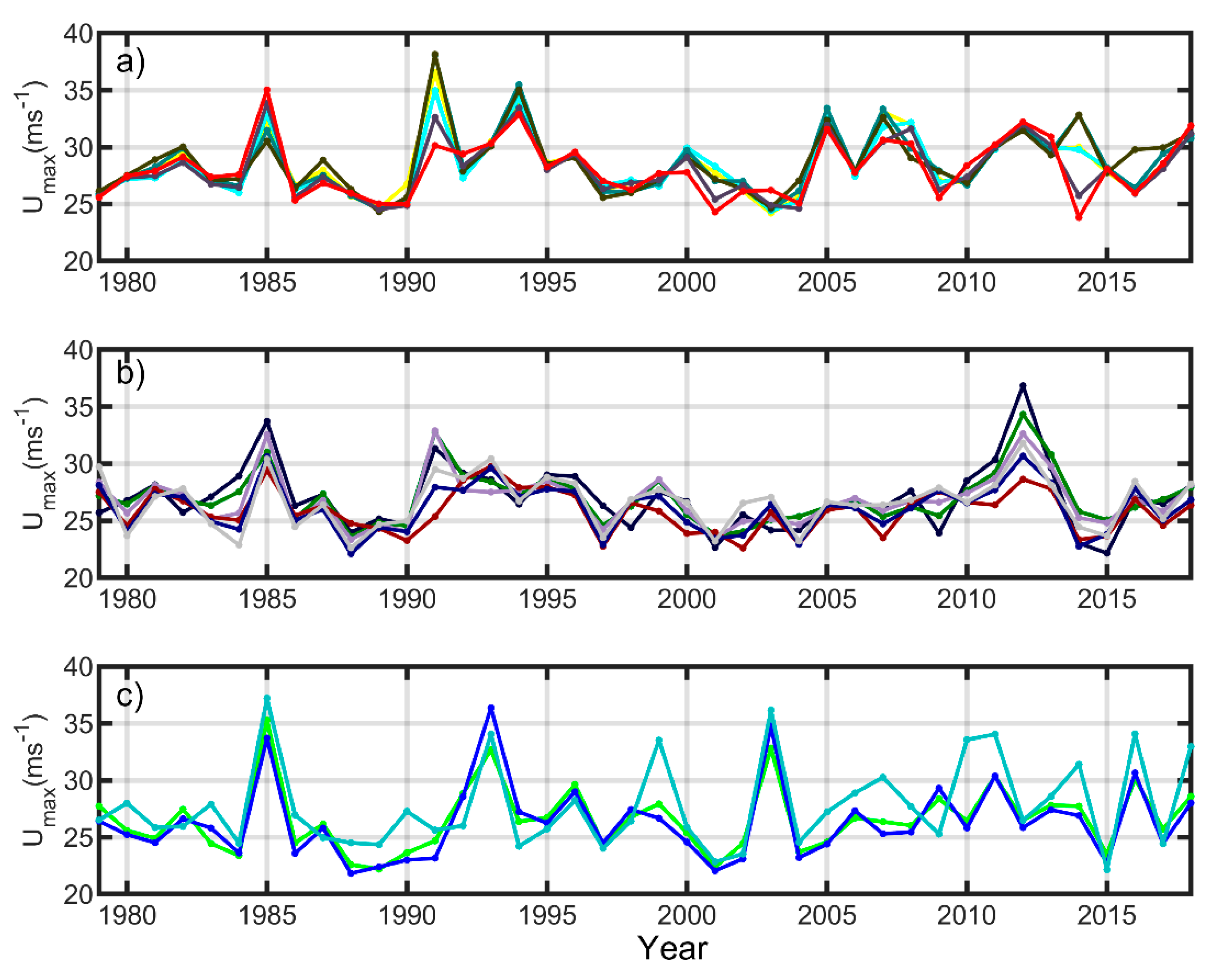
U40 is defined as the maximum of the annual maximum wind speeds at 100 m height for each LA derived from the 40-year record of ERA5 data. U40 from ERA5 at all LA over 1979–2018 are in the range 21.8–38.1 ms−1 (Figure 2). Only a few LA or years exceed the Turbine class III 50-year return period wind speed of 37.5 ms−1. Recall the record here is 40 years long and also that maximum values are likely to be higher for individual locations than they are over ≈31 × 31 km grid cells due to spectral smoothing. The highest wind speed at 100 m height is 38.1 ms−1 for LA 3 and 4 (which use the same ERA grid cell) and LA 5. These are the most northerly and easterly of the LA grid cells, but all LA in the north group and LA 8 (off NY state) have a 40-year maximum wind speed close to or above 35 ms−1. The central group of LA 9–13 (off the coast of NJ, DE and MD) have slightly lower Umax between 29.8–34.3 ms−1 while the 40-year maximum wind speed further south off the coast of NC and VA in LA 13–16 increases to above 35 ms−1. This is reflected in the mean maximum wind speed of above 28 ms−1 for the northern LA and from 25.9–27.8 ms−1 for the central and southern group of LA (Figure 2).
Of the 16 LA, LA 14 and 15 off the coast of North Carolina have the highest frequency of wind speeds at 100 m a.s.l. in excess of 33 ms−1 in the ERA5 reanalysis dataset. These LA were also identified as exhibiting the greatest probability (of 0.3/year) of wind speeds of 33 ms−1 or greater (at 10 m height and 1 min averaging time) based on a catalogue of simulated hurricanes while the coast of DE had the lowest probability of exceeding this threshold of 0.17/year [28].
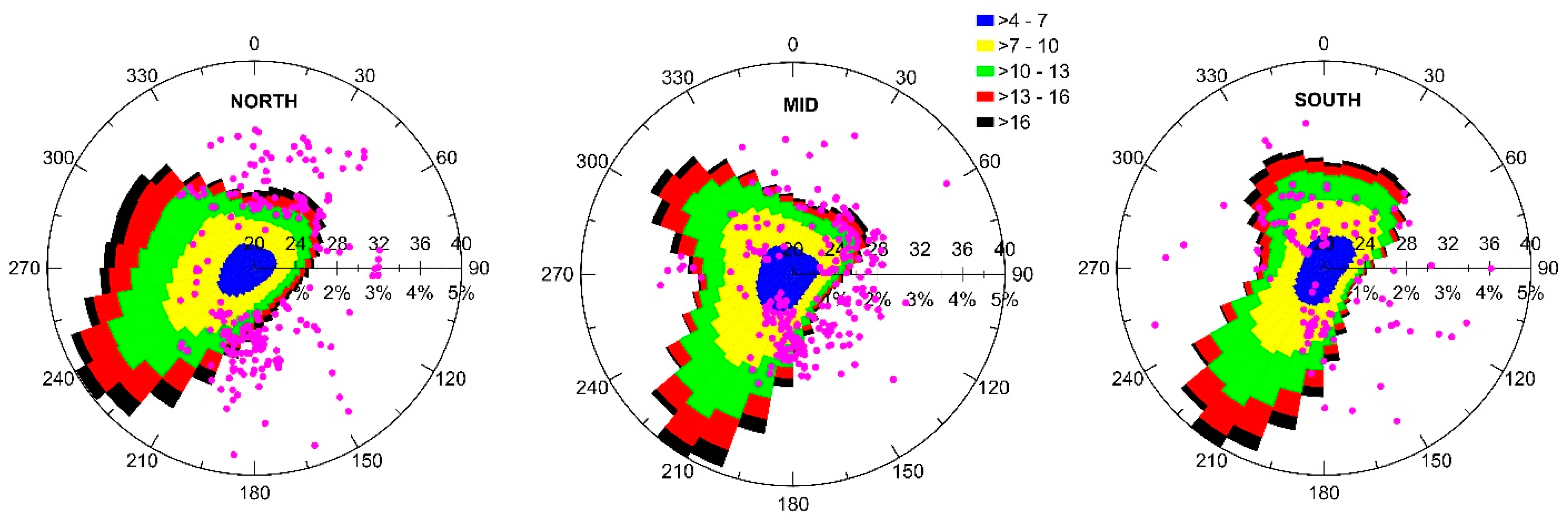
ERA5 hourly wind output at 100 m a.s.l. from the 16 LA exhibit clear spatial variability in the prevailing wind climates (Figure 3, Table 2). The northern LA to the south of Massachusetts have a long over sea fetch to the southwest (Figure 1) and the wind rose is dominated by flow from the southwest, particularly in the power producing wind speeds (Figure 3). Winds from the west and southwest also exhibit the greatest frequency of the highest wind speeds (>16 ms−1), but the annual maximum winds are more frequently associated with southerly and/or north/northeasterly with relatively few Umax from the west (Figure 3). The LA in the mid-group exhibit a strongly bi-directional wind rose with southwesterly and northwesterly wind directions being most prevalent, while the southerly LA group exhibit a dominance of southwesterly flow and a relatively low frequency of westerly and northwesterly flow (Figure 3). However, there is a much greater prevalence of southeasterly flow associated with Umax (Figure 3). For the mid LA from NY to MD, the dominant wind direction is south/southwest, with a secondary peak from the northwest direction. Annual maximum wind speeds are lower than those from the northern LA (Figure 2 and Figure 3) and again exhibit a relatively high frequency of southerly and southeasterly directions particularly for the largest Umax values. There are a higher number of Umax from east than for the north LA. For the three LA in the south of the domain there is distinct bidirectionality with south/southwest and north/northeast components to the wind rose (Figure 3), and a much higher frequency of southeasterly directions in Umax with relatively few annual maxima from westerly and southwesterly directions.

3.2. Sources of Intense and Extreme Wind Speeds

High wind speeds in the northeastern US typically derive from the progression of mid-latitude or tropical cyclones [67]. Dominate cyclone genesis and cyclone tracks are; Alberta Clippers (AC) that form in the lee of the Canadian Rockies and track east, Colorado Lows (CL) that form in the lee of the Rocky Mountains near the U.S. state of Colorado and track northeast, moving northwest, and Tropical Cyclones (TC) that form in the tropical Atlantic and track north up the U.S. east coast. These cyclones can re-intensify as they move offshore and/or retrograde (move west) onshore in the form of Nor’Easters [67].
Typically, TC produce the highest wind speeds and are described as hurricanes if wind speeds at 10 m a.s.l. exceed 33 ms−1 and major hurricanes if wind speeds exceed 49 ms−1. Hurricanes have return periods for passing within 58 miles of the coast ranging from 13–20 years for most of the North Atlantic coast north of NC, increasing to 30 years north of MA but decreasing to 5–7 years off NC (https://www.nhc.noaa.gov/climo/#returns. Date of access: 20 November 2020). Return periods for major hurricanes are 44–76 years for the coast north of NC decreasing to 16–25 years along the NC coast. Dates of some annual maximum wind speeds manifest in ERA5 are clearly linked to historical wind storms primarily, but not exclusively, of tropical origin. For example, the year 1985 stands out in the ERA5 records as producing the highest or second highest maximum wind speeds in the time series of maximum wind speeds for all LA (Figure 2). These extreme wind speeds are associated with Hurricane Gloria (16 September–2 October 1985) which tracked along the Atlantic coast [68]. High wind speeds in the northeast in 1991 are linked to Hurricane Bob (18–19 August 1991) which hit the Carolinas, skirted the Atlantic coast, and made landfall in Rhode Island (16–29 August 1991) and with an intense Nor’-easter on 31 October 1991 [69]. The highest wind speeds in the central LA cluster occurred in 2012 linked to Hurricane Sandy (October 22–November 2 2012) [70]. The southern LA off VA and NC have eight occurrences of annual maximum wind speeds over 33 ms−1 and three over 35 ms−1 in 1985 (as above), in 1993 associated with a March ‘superstorm’ and 2003 Hurricane Isabel (6–20 September 2003) which made landfall in North Carolina [67].
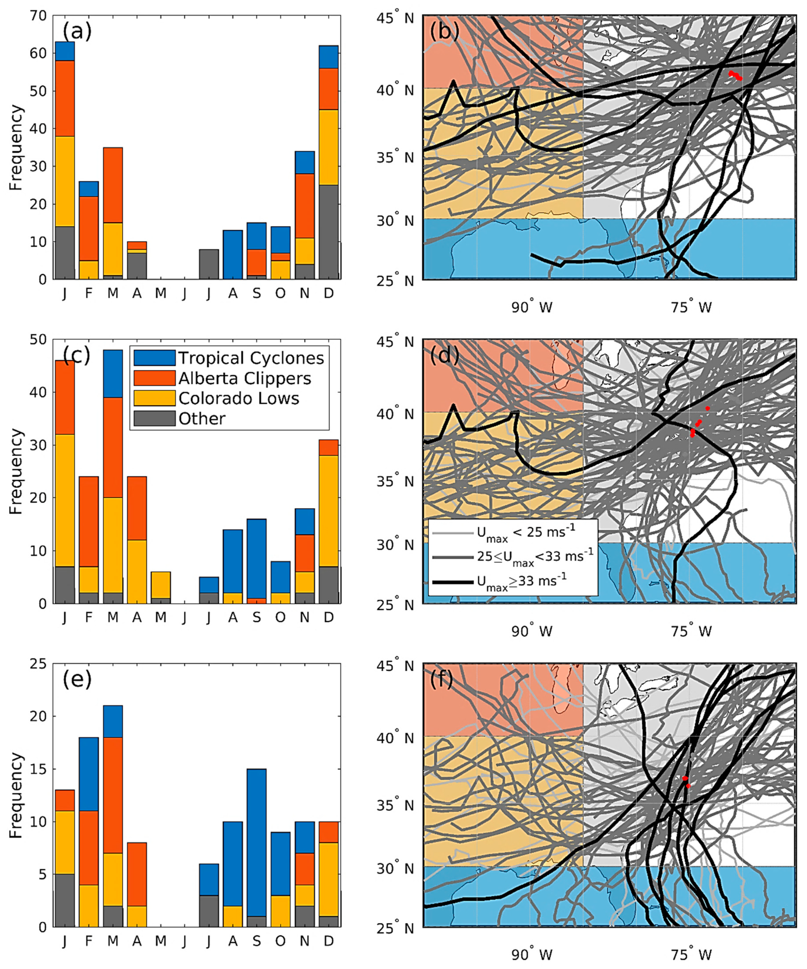
Analyses of the cyclone genesis and tracking based on the ERA5 output confirm expectations based on previous research and indications from the analysis of the time series of annual maximum wind speeds and indicate marked differences in the frequency of TC passages over the different LA. The LA in the north (LA 1–7) are seldom impacted by TC and experience their annual maximum wind speed mainly in the winter months arising from both AC and CL (Figure 4). The mid LA group (LA 8–13) also tend to experience highest wind speeds (and thus Umax) during the winter months that are more frequently associated with passages of CL, but AC are an important contributor to Umax. In the mid group TC are also responsible for a fraction of the Umax values and most frequently occur in the months from July to October. The south group (LA 14–16) have a much higher frequency of annual wind maxima from TC in July through November, while also experiencing annual wind maxima in January and February from AC and CL. This explains to some degree the finding that mean wind speeds in general are lower in the south LA (Table 2), but the annual maxima can be as high as those in the north LA. Thus, although past research has tended to focus on the hurricane threat to the offshore LA along the U.S. east coast the highest wind speeds in the northern LA tend not to be associated with TC. Indeed, the likelihood of impact from a TC is relatively small and the TC that do impact these LA are not associated with atypically intense wind speeds (Figure 4).

3.3. Results from the Different Methods of Estimating U50

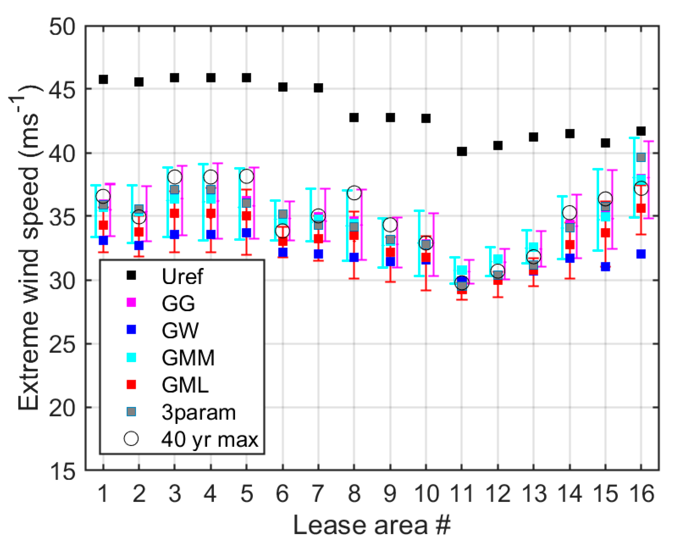
Uref is not a prediction of U50 per se but a conservative value to be used within the wind turbine standards. As such it fulfils that role, exceeding U50 estimates from the other methods and the maximum wind speed observed during the 40-year record (U40) values by over 2 ms−1 in ERA5 output from every LA and up to 10 ms−1 at most LA (Table S1). The gap between Uref and U50 tends to narrow moving from the northern LA southwards consistent with the decrease in annual mean wind speeds (Table 2), while U40 values in the southern LA exceed those in the mid LA and are comparable to those in the northern LA (Figure 5, Table S2).
U50 at 100 m a.s.l. across the 16 LA as derived using ERA5 range from 30 to 40 ms−1 (Figure 5, Table S2). Spectral smoothing in numerical models applied with 25 km grid resolution was estimated to result in underestimation of extreme wind speeds over seas in northern Europe by about 11% relative to anemometer measurements on meteorological masts [39]. The longer temporal averaging inherent in the ERA5 model time step will likely yield a smaller reduction of 2–3% in the maximum wind speed relative to a 10-min averaging period employed in the IEC standard [40]. Assuming these corrections are additive and are applicable to the ERA5 output the implied pseudo-point U50 estimates range from 34 to 46 ms−1. For comparison U50 estimates derived from measurements at two offshore/coastal locations in Europe; Høvsøre in Denmark, and the FINO offshore platforms in the North Sea are 42.8 ms−1 and 35.3 to 39.3 ms−1, respectively. Thus, based on this assessment for many of the offshore LA in the mid and northern LA groups the expectation is that extreme wind speeds will be comparable to those experienced near major offshore wind turbine arrays in northern Europe.
The spatial variability in U50 across the 16 LA are generally consistent across the different distribution fitting approaches (Figure 5, Table S2). Sampled across the 16 LA, all U50 estimates lie within a range of 7.6 ms−1 and excluding the two most southerly LA, all U50 values lie within 3.6 ms−1 of each other (Figure 5). For comparison, the bootstrapped 95% confidence intervals on U50 from the GML method at the 16 LA are 2.5 to 8.6 ms−1. Equivalent bootstrapped 95% confidence intervals on U50 from GG and GMM are 3.3 to 11.4 ms−1 and 3.9 to 12 ms−1, respectively. In all cases the southern LA exhibit the widest confidence intervals. Since the data of the boot-strapped samples exhibits larger confidence intervals than the difference in U50 from the statistical methods, this may imply that the selection of data periods used to derive U50 is a larger source of uncertainty than the parameter fitting method. For LA 15 and 16 this is not the case as the GW method gives low estimates of U50 that lie outside of the confidence interval generated by bootstrapping.
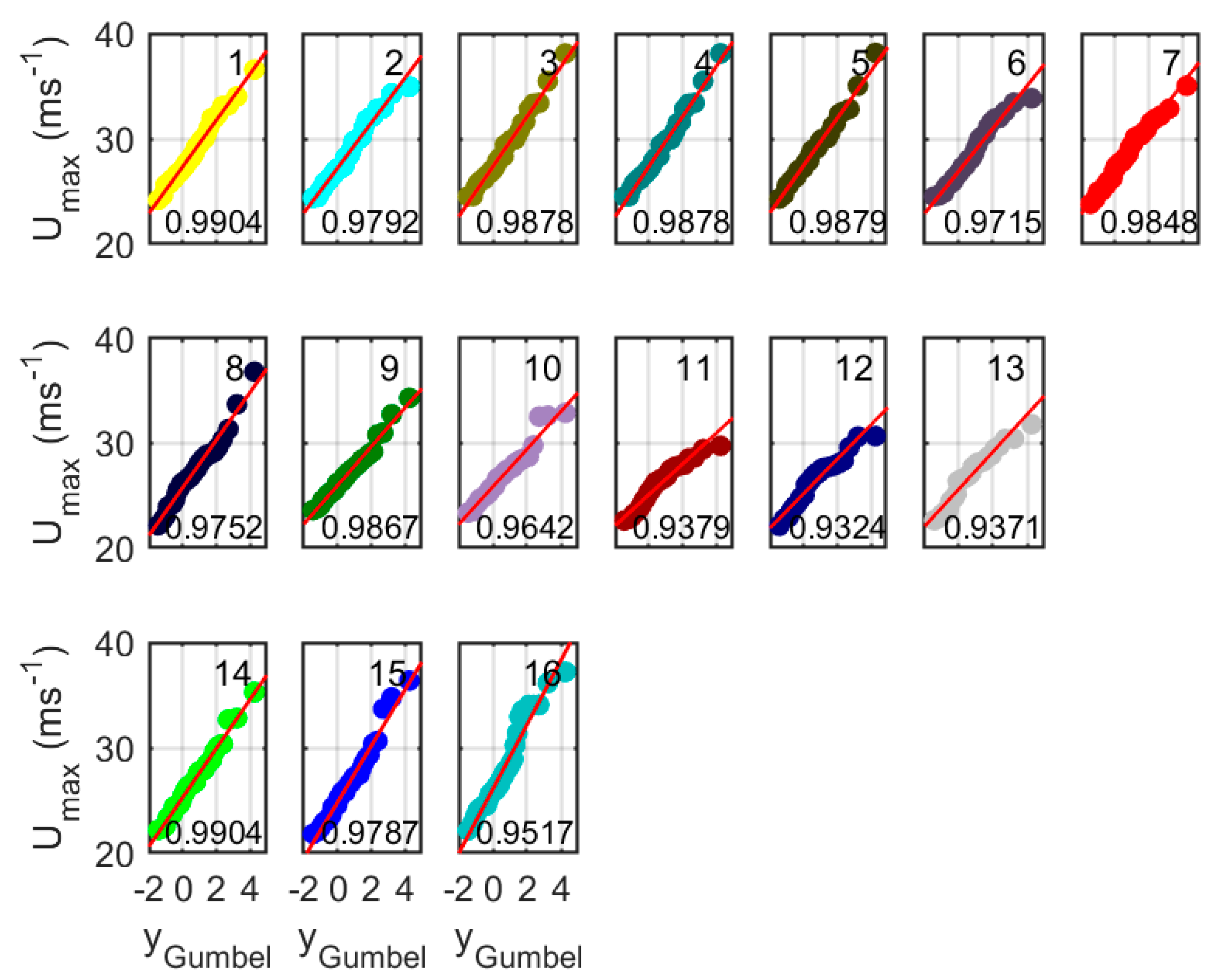
The GG, GMM and GML methods use fits to the maximum annual wind speed to determine U50 while GW use fits to the whole wind speed distribution. GG and GMM give very similar values for U50 at all LA. U50 determined from GW give consistently the lowest values. The Weibull fit is intended to fit the bulk of the whole distribution and is not tailored for the tail of the distribution. Hence GW tends to give predictions which are low compared to the other estimates, although they lie within the bootstrapped 95% confidence intervals of the GML method for all LA except LA 15 and 16. GML estimations are higher than GW estimates but lower than estimates from GG/GML. For the GG method, the coefficient of determination (r2) of the linear fit between rank-ordered annual maxima and the reduced variate generally exceeds 0.97 for the northern LA indicating a high degree of linearity in the relationship (Figure 6). The lowest values (r2 < 0.94) are evident in data from the southernmost LA (11–13). Thus, there is some evidence of mixed wind climates in the linear fits in individual LA [71] with Umax deviating markedly from the fitted straight line, particularly for the mid area LA (10, 11, 12) which are more coastal. LA 1–5, 8 and 14–16 may be subject to occasional extreme winds from the paths of tropical cyclones (Section 3.2). LA 6,7 and 9–13 have a minimum distance (of the central location) to the coast to the west/southwest of around 30 km (Table 2) which may also have an impact on the wind speeds in terms of their adjustment to the lower roughness and temperature of the sea surface [72]. The minimum distance for LA 1,2 is to the coastline to the north (a less favored direction in terms of frequency). The remaining LA are 42–65 km east of the coastline.
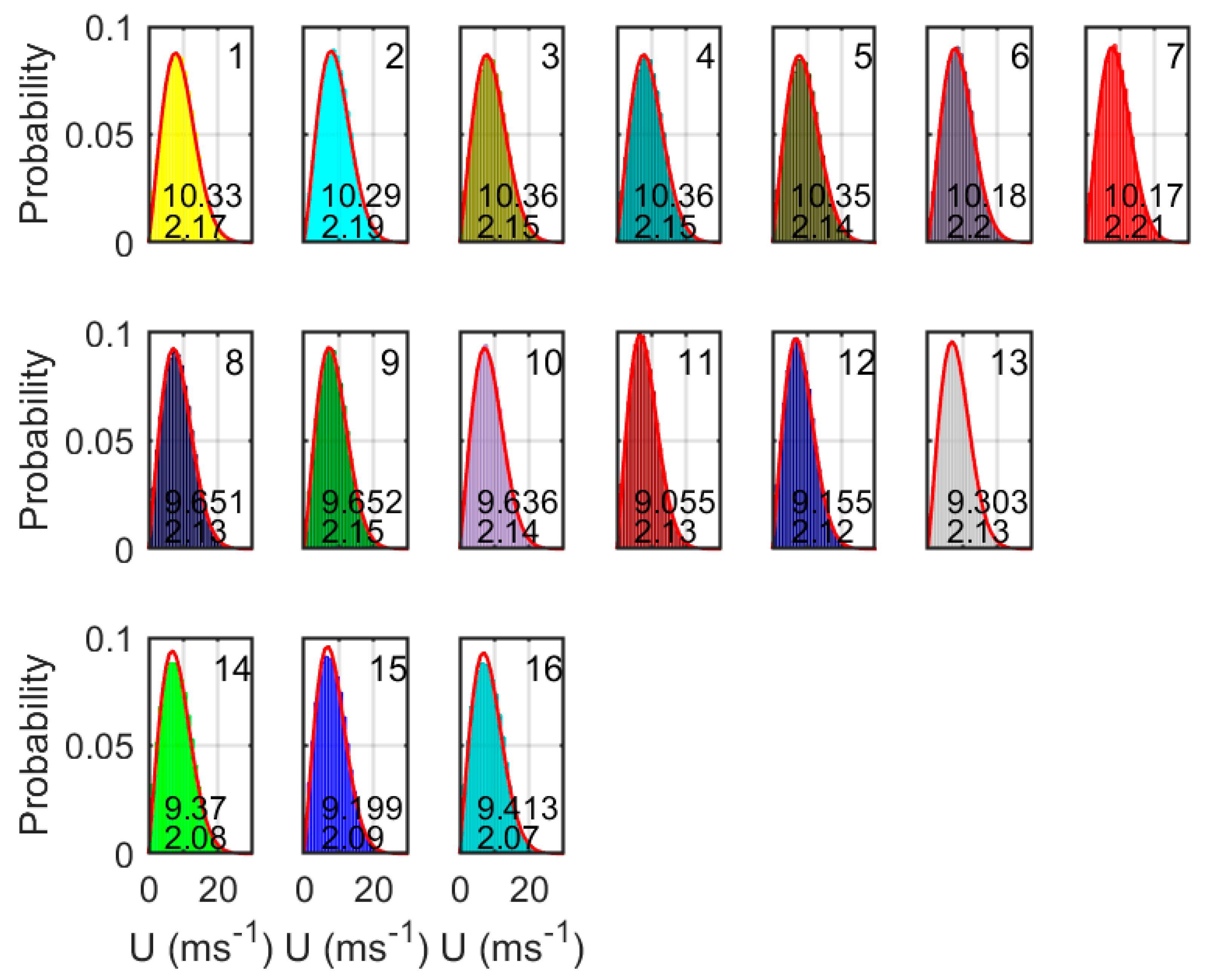
The marginal probability density function of once hourly wind speeds in LA are generally well described by the two-parameter Weibull distribution (Figure 7, Table S1). The LA all show similar Weibull shape parameters (k) of 2.07–2.21, which are typical for offshore conditions [73] with slightly less peaked distributions (lower k) in the southern LA. The scale factors are highest in the northern LA and lower by about 0.7 ms−1 in the southern LA. The scale factors for the mid LA vary the most from 9.06 to 9.66 ms−1. Despite the relatively good fit of the hourly data to a two-parameter Weibull distribution U50 estimates derived by extrapolation of the Gumbel distribution parameters from the Weibull parameters tend to be negatively biased relative to those from the other methods (Figure 5).
Visualization of the two-parameter GEV (Gumbel) fits to annual maximum wind speeds where the parameters are derived using MLE methods indicates the fits are insufficiently peaked (Figure 8). This may be partly because some LA (notably 8,9,14–16) show evidence of being bimodal (Figure 8), indicating a mixed wind climate and that the Umax values derive from two distinct sources (e.g., TC and CL in the southern LA, Figure 4). The 3-parameter GEV is visually a superior fit to the annual maxima (Figure 8), however, the 95% confidence interval on the shape parameter in most of the fits includes zero. The exceptions are for LA 11–13 which have negative shape parameters which means they are type 3 Fisher–Tippett distributions. LA 7&8 are also type 3 Fisher–Tippett distributions, but the confidence intervals cross zero. The remaining LA all have positive shape parameters (Type I) with confidence intervals that cross zero. Although Figure 8 offers evidence that a 3-paramater GEV is a better representation of the sample of annual maximum wind speeds at most LA, as shown in Figure 5 the 50-year RP wind speed estimates from the two parameter GEV (Gumbel) and three parameter GEV fits do not differ greatly.
The three parameter GEV method estimates the highest values for U50 at the majority of LA, with similar values to U50 from GG and GML except for LA 11–13. For the north LA and LA 9–10 the range of estimates for U50 are within the 95% confidence intervals from GML. U40 from the ERA dataset is slightly higher than most estimates for LA 1–10 (excluding LA 6). For LA 11–16 U40 is lower than the estimates of U50 (excluding LA 14). Estimates for LA 11–13 have a smaller range of confidence intervals and have the lowest values of U40 and the lowest values of U50 estimated from all methods. Note that the nearest land areas to these LA have the lowest return period (5–7 years) for hurricane wind speeds (33 ms−1) (https://www.nhc.noaa.gov/climo/#returns. Date of access 20 November 2020). This is consistent with the description of extreme winds over the LA described in the paper, namely that the south LA experience Umax that are typically lower than the other LA but can be impacted by TC bringing hurricane wind speeds.

3.4. Wave Heights

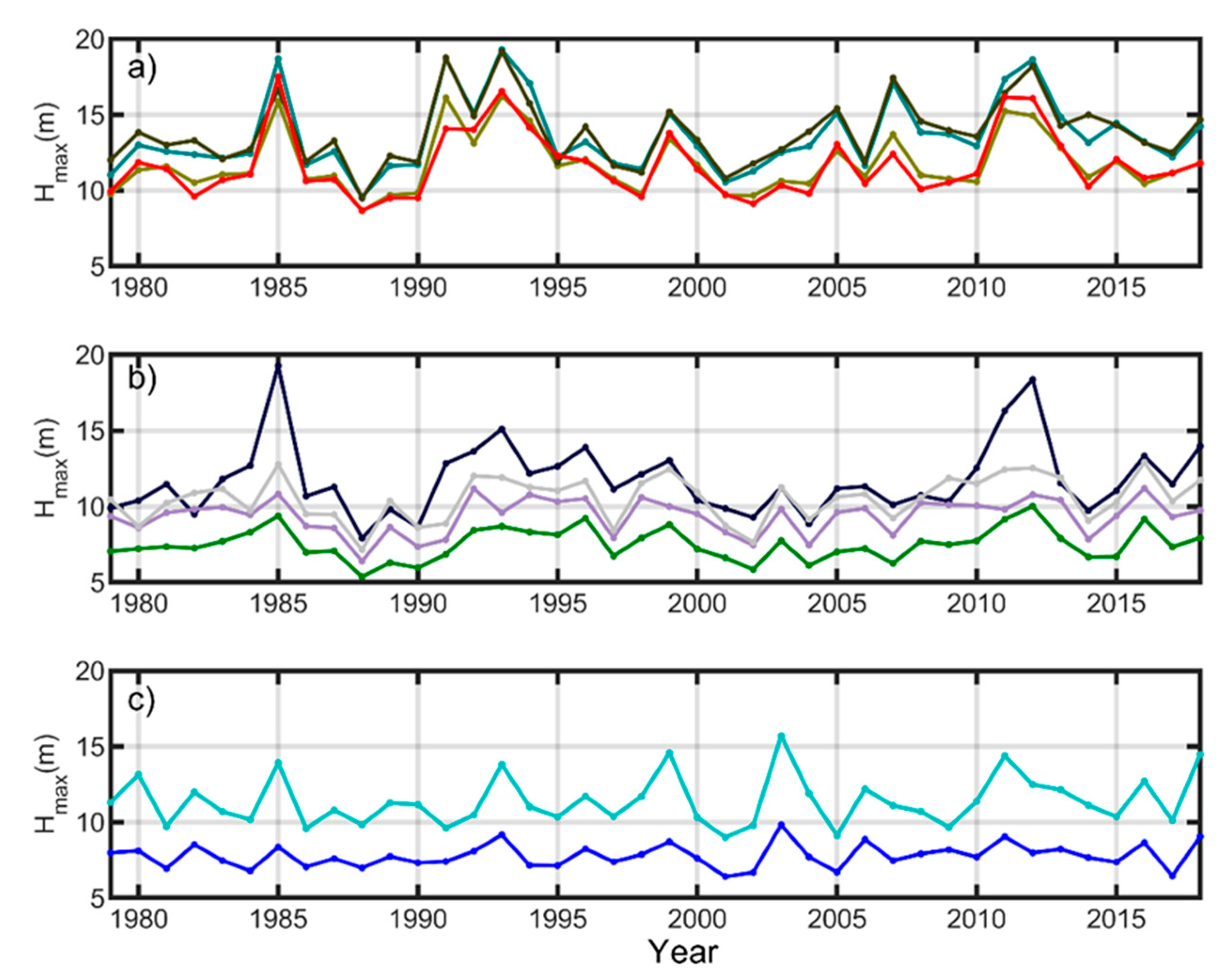
As with Umax, there is substantial year to year variability and a marked north to south gradient in annual maximum Hmax with maximum values of almost 19 m in the northern LA while in the south LA the maximum values are generally below 15 m, and in LA 15 no annual maximum Hmax exceeds 10 m (Figure 9). There is more spatial variability in Hmax than in the annual maximum values for wind speed, particularly in the mid-LA groups. For example, LA 8 exhibits substantially higher Hmax values in most years than the other LA in that group. Annual maximum Hs (not shown) exhibit similar spatial variability but lower absolute values (annual maxima range from 2–11 m). There is substantial co-occurrence in time of maximum annual wind speeds and Hmax at all of the LA (Table 4) which implies that in many years cyclones that are responsible for intense wind speeds are also responsible for generating the largest waves. In most LA approximately half of years exhibit the highest values of both Umax and Hmax occur within a 6 h time window (Table 4).
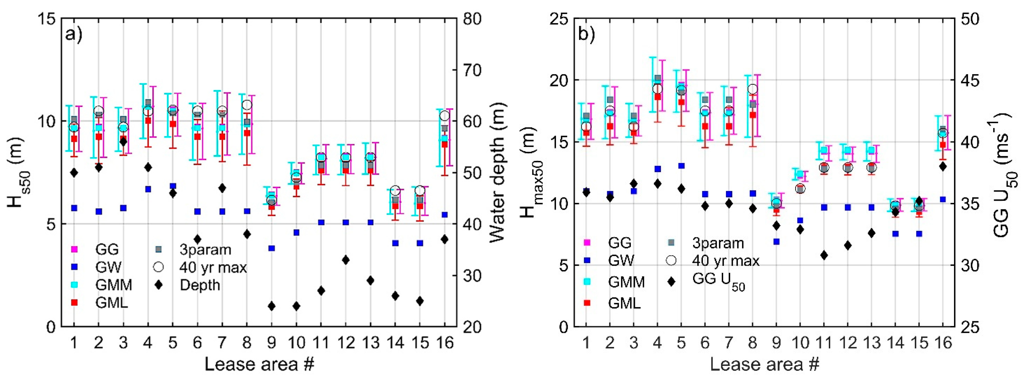
A range of marginal distributions has been applied to Hs including log-normal and Weibull distribution [74], and there is evidence that a three-parameter Weibull distribution is necessary to describe wave data [75]. Past research has employed a two-parameter Gumbel distribution for extreme Hs [76], and in analysis of the ERA5 wave data it appears to generate very similar values to those from the three-parameter GEV (Figure 10). Fifty-year return period significant wave height and maximum wave height (Hs50 and Hmax50, respectively) from the different distribution fits are generally consistent (Figure 10). The lack of agreement with estimates derived using the extrapolation from a two-parameter Weibull fit may reflect a relatively poor fit of the 3-hourly wave data to this parent distribution. The r2 values for the GG fits to the samples of annual maximum Hmax and Hs are greater than 0.93 at every site. All Hs50 values expect from those using GW lie within the bootstrapped 95% confidence intervals on the GG, GML and GMM estimates (Figure 10). In all LA the confidence intervals on one or more of Hs50 estimates include the maximum Hs reported in the 40 years of ERA5 reanalysis output (Figure 10). Excluding the GW method, as with the extreme wind speeds, the bootstrapped 95% confidence intervals on the 50-year return period wave properties are wider than the range between estimates from the different GEV and/or parameter fitting methods. This indicates that resampling with replacement the 40-year record to generate many simulated samples yields larger variability in derived Hs50 and Hmax50 than arise from application of the different distributional forms.
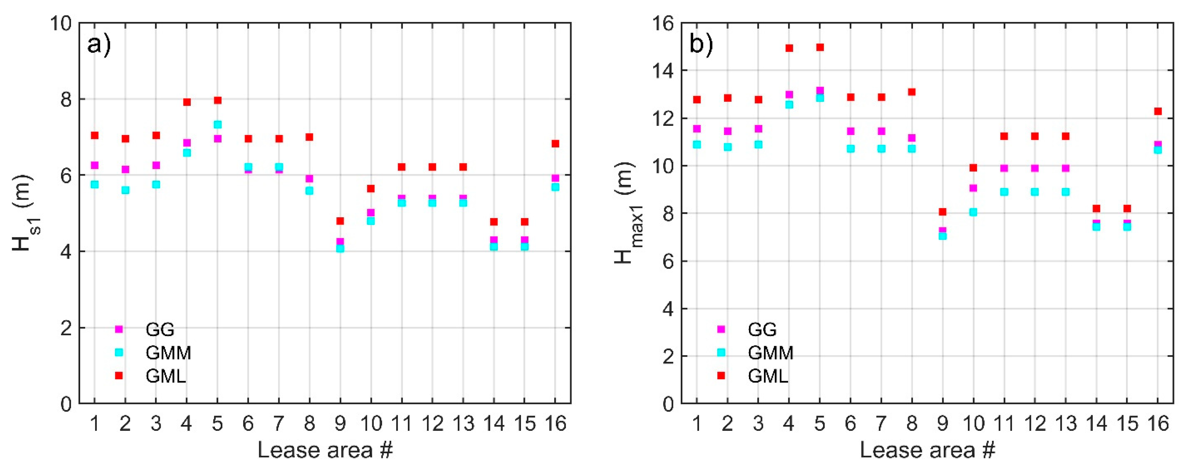
The lowest Hs50 are just below 6 m at LA 9 and LA 14,15 (same grid cell) derived using the GML method with slightly higher values estimated by GG or GMM. The 3 parameter GEV estimates give the highest estimates. However, as is the case for U50, the confidence intervals on the shape parameter for Hs50 cross zero for all LA except LA 9 and 10 which are negative. Most LA have slightly negative shape factors for Hs50 that are indistinguishable from zero. Only LA 5 and LA 11–13 have positive shape factors (with confidence intervals that include zero). The values of both Hs50 and Hmax50 are strongly associated with water depth and also to U50. The coefficient of determinations for Hs50 and Hmax50 (from GG) with linear fits of water depth are both 0.66.
Estimated values of Hs50 are consistent with a study based on hindcast data for the period 1978–2008 for most of the US Atlantic east coast that indicated values of 5 m in the coastal zone increasing to 10 m in deeper water [77]. The values for 50-year return period value of Hs are highest in the north LA where they range between 9 and 11 m. These values are higher those derived in an analysis of five buoys in the Gulf of Maine (to the north of the current LA) that indicated extreme Hs with a 50-year return period of 4.7 to 9.8 m [64]. The Hs50 estimates for the northern LA are also above those reported around the coast of Spain that ranged from 4.5 to 8.2 m [78] and for most of Danish waters that have offshore wind farms [79]. Model results indicate Hs50 > 9 m in the more open waters of the North Sea west of Denmark, where U50 at 100 m height are modelled to exceed 40 ms−1.
The spatial variability in Hmax50 across LA is similar to Hs50 (Figure 10). The largest values are just over 20 m from the GG method and the 3 parameter GEV for LA 4 and above 9.8 m for every LA using that method. To contextualize the extreme wave height estimates it is worthy of note that the IEA 15 MW offshore reference wind turbine indicates a height of 15 m above mean sea level for the transition piece [80]. Application of the GG method yields linear fits have an r2 value above 0.95 for all LA except 10–13 where r2 = 0.84 for LA 10 and 0.87 for LA 11–13. Although the Weibull fits are slightly less peaked for Hmax50 than they are for Hs50, the two-parameter Weibull distribution is generally a poor fit to the Hmax time series data, and thus extrapolation of the Gumbel distribution parameters yields Hmax50 that are substantially negatively biased relative to those from the other methods (Figure 10). The GML two parameter plot is a good fit to the more peaked distributions of Hmax50 for LA 9–15 and less so for the northern LA. Consistent with analyses of wave data from Ireland [59], the shape parameter in the three-parameter GEV fits to samples of annual maximum Hmax vary around zero. The shape parameter from the 3 parameter GEV distribution is mostly positive (for LA 1–4, 6–8 and 16) except LA 5,9 and 14,15 although for all of those LA, the 95% confidence intervals on the shape parameter include zero. For LA 10–13 the shape factor is negative and the confidence intervals do not cross zero implying the three-parameter GEV fit to annual maximum Hmax is superior to the two parameter Gumbel.
One year return period values for Hmax and Hs are also used in the design process and so were computed (Table 4 and Figure 11). The IEC standards note that expected ratios of the extreme wave height Hmax with a given return period (50-years or one year) are 1.9–2.0 times the significant wave height Hs with the same return period in deep water. Data from the ERA5 reanalysis indicate that for all 16 LA that ratio for the 50-year return periods are 1.5–1.9. For the one-year return period, the ratios range from 1.7–1.9 for all methods used (Table 4).

4. Discussion

The ERA5 dataset provides a nearly homogeneous data record for analyzing extreme wind speeds and waves in offshore areas where in situ data are sparse. In addition to the relatively high spatial and temporal resolution, ERA5 includes wind speeds for 100 m height which is representative of the hub-height of wind turbines currently being deployed offshore. Hence, ERA5 output is used here to develop first estimates of extreme wind speeds and wave conditions in the 16 lease areas (LA) selected by the Bureau of Ocean Energy Management for the development of offshore wind energy along the U.S. east coast.
The annual maxima wind speeds at 100 m a.s.l. tend to be higher in the northern LA (south of the U.S. states of Massachusetts and Rhode Island) than those off the coast of New York, New Jersey, Delaware, and Maryland (the mid-LA), possibly because these are closer to the coastline (Table 2). The southern LA off the coast of Virginia and North Carolina have lower mean annual maximum wind speeds but also experience occasional very high annual maxima that are associated with tropical cyclones. The highest annual maximum wind speed at 100 m a.s.l. over the 40-year time period from any ERA5 grid cell that contains an offshore LA is 38.1 ms−1, and it impacted the northern LA. Using approximations to account for spectral truncation of the ERA5 model and temporal averaging of ~12–20 min versus 10 min in the IEC standards this equates to a wind speed of 43.4 ms−1. Tropical cyclones are observed to impact the LA during July to November, and are more frequently the cause of annual wind maxima in the southern LA than either Alberta Clippers or Colorado Lows. Extratropical cyclones associated with AC and CL are more frequently associated with annual wind maxima at the northern and mid LA and are more frequently experienced in the cold season.
A number of different methods are available to estimate extreme wind speeds. While most rely on fitting distributions (two- or three-parameter GEV) to the annual maxima with estimation of the distribution parameters from a graphical approach, method-of-moments or maximum likelihood estimation, it is also possible to derive the Gumbel parameters from Weibull distribution parameters derived by fitting the parent distribution of hourly wind speeds. Although this Gumbel-Weibull method gives the lowest estimates for U50 it may be expedient where the time series of wind speeds that are available for analysis are highly fractured and/or of insufficient duration to generate a robust sample of annual maxima. For most LA, U50 values estimated by the different methods lie within the 95% confidence intervals generated on the Gumbel Method of Moments, Gumbel Maximum Likelihood and/or Gumbel-graphical methods. All of the U50 estimates are at least 2 ms−1 below the Uref wind speeds derived as specified in the IEC standard as five times the mean annual wind speed, and at most of the LA this difference exceeds 5 ms−1, indicating Uref is highly conservative of U50.
It is important to note that we have computed and present independent exceedance values of wind and waves at offshore LA in that univariate probability distributions are fitted independently to each parameter. We have focused our analyses on understanding the causes of the intense wind speeds spatial variability in extreme values and uncertainties on the long return period estimates that arise due to the precise data period used (via the bootstrapping) and the method used to fit the GEV distributions. Naturally, all structural reliability assessments require joint distributions [81]. In that context it is worthy of note that analyses presented herein suggest a relatively high frequency of co-occurrence (within a 6 h time window) of low frequency, high magnitude values of wind and wave parameters.

5. Concluding Remarks

U50 values derived from ERA5 output at heights characteristics of wind turbine hub-heights range from 30 to 40 ms−1. Lease area 16 has the highest estimated U50 value of 39.7 ms−1 which derives from the 3-parameter GEV. Extreme wind speeds in the southern LA that are impacted by tropical cyclones are more difficult to characterize and Uref is much less likely to be conservative [22]. After applying a correction factor to account for missing variance of 1.14, the U50 values for many of the LA appear to indicate that wind turbine class II (with a reference wind speed of 42.5 ms−1) may be adequate. However, it is possible that corrections for spectral smoothing from Europe may not be appropriate to the flow conditions along the U.S. east coast and/or that the ERA5 reanalysis exhibit stronger spectral smoothing than the numerical modelling on which these approximations were derived.
For wave height characterization, the maximum wave height and significant wave height show similar behavior. Consistent with the higher wind speeds in the northern LA both tend to be slightly higher in the northern LA. The highest annual maximum wave height in the ERA5 dataset is over 19 m while the highest Hmax50 estimate is over 20 m. Hs50 lies between 9–11 m for most of the northern LA. For both these metrics, wave characteristics at LA 8 and 16 are similar to the northern LA. The lowest values for Hs50 are in LA 9, 14, and 15 where Hmax50 is around 10 m and Hs50 is around 6 m. As with extreme winds, any of the methods used give estimates which lie within the 95% confidence intervals, except the Weibull method which does not appear to be suitable for extreme wave characteristics.

Supplementary Materials

The following are available online at https://www.mdpi.com/1996-1073/14/4/1053/s1, Table S1: Mean maximum wind speed, Weibull shape and scale parameter, mean wind speed and standard deviation for each LA, Table S2: Maximum estimated U50 and 40 year observed maxi-mum wind speed at each site (ms−1).

Author Contributions

R.J.B. and S.C.P. jointly developed the concept and analysis strategy, ran the analysis and generated the figures. K.E.D. and E.J.R. contributed to initial research. F.L.L. ran the storm track code and generated the associated analysis and figure. R.J.B. and S.C.P. wrote the manuscript with input from F.L.L., E.J.R., and K.E.D. All authors have read and agreed to the published version of the manuscript.

Funding

This work was supported by grants from the U.S. Department of Energy (DoE) Office of Science (DE-SC0016438 and DE-SC0016605). Additional support derives from the U.S. Department of Energy’s Office of Energy Efficiency and Renewable Energy (EERE) under the Wind Energy Technologies Office Award number DE-EE0008390 and the New York State Energy Research and Development Authority (NYSERDA) via the National Offshore Wind Research and Development (NOWR&D) consortium (award 147505). NYSERDA has not reviewed the information contained herein, and the opinions expressed in this report do not necessarily reflect those of NYSERDA or the State of New York or the U.S. Department of Energy. The research used computing resources from the National Science Foundation: Extreme Science and Engineering Discovery Environment (XSEDE) (allocation award to SCP is TG-ATM170024). Funding for student participation was provided by Engaged Cornell.

Institutional Review Board Statement

Not applicable.

Informed Consent Statement

Not applicable.

Data Availability Statement

Copernicus Climate Change Service (C3S) (2017): ERA5: Fifth generation of ECMWF atmospheric reanalyses of the global climate. Copernicus Climate Change Service Climate Data Store (CDS), date of access 26 August 2020. https://cds.climate.copernicus.eu/cdsapp#!/home Bathymetry data were downloaded from GEBCO Compilation Group (2020) GEBCO 2020 Grid (doi:10.5285/a29c5465-b138-234d-e053-6c86abc040b9).

Acknowledgments

Thanks to Gunner Christian Larsen of the Danish Technical University for provision of useful information.

Conflicts of Interest

The authors declare no conflict of interest.

References

  1. WindEurope. Wind Energy in Europe Trends and Statistics 2019. 2020, p. 24. Available online: https://windeurope.org/wp-content/uploads/files/about-wind/statistics/WindEurope-Annual-Statistics-2019.pdf (accessed on 27 February 2020).
  2. Jansen, M.; Staffell, I.; Kitzing, L.; Quoilin, S.; Wiggelinkhuizen, E.; Bulder, B.; Riepin, I.; Müsgens, F. Offshore wind competitiveness in mature markets without subsidy. Nat. Energy 2020, 5, 614–622. [Google Scholar] [CrossRef]
  3. Bosch, J.; Staffell, I.; Hawkes, A.D. Global levelised cost of electricity from offshore wind. Energy 2019, 189, 116357. [Google Scholar] [CrossRef]
  4. WindEurope. Offshore Wind in Europe Key Trends and Statistics; 2020; p. 40. Available online: https://windeurope.org/wp-content/uploads/files/about-wind/statistics/WindEurope-Annual-Offshore-Statistics-2019.pdf (accessed on 27 February 2020).
  5. Musial, W.; Heimiller, D.; Beiter, P.; Scott, G.; Draxl, C. 2016 Offshore Wind Energy Resource Assessment for the United States. Technical Report NREL/TP-5000-66599. 2016; p. 88. Available online: https://www.nrel.gov/docs/fy16osti/66599.pdf (accessed on 16 July 2020).
  6. EIA. Electric Power Annual 2019 October 2020; US Energy Information Administration, 2020; p. 240. Available online: https://www.eia.gov/electricity/annual/pdf/epa.pdf (accessed on 22 November 2020).
  7. DeCastro, M.; Salvador, S.; Gómez-Gesteira, M.; Costoya, X.; Carvalho, D.; Sanz-Larruga, F.; Gimeno, L. Europe, China and the United States: Three different approaches to the development of offshore wind energy. Renew. Sustain. Energy Rev. 2019, 109, 55–70. [Google Scholar] [CrossRef]
  8. BOEM. Coastal Virginia Offshore Wind Project (CVOW). Available online: https://www.boem.gov/renewable-energy/state-activities/coastal-virginia-offshore-wind-project-cvow (accessed on 22 November 2020).
  9. AWEA. US Offshore Wind Energy Status Update OTOBER 2019. 2019. Available online: https://www.awea.org/Awea/media/Resources/Fact%20Sheets/Offshore-Fact-Sheet-Oct-2019.pdf (accessed on 22 July 2020).
  10. BOEM. BOEM Governing Statutes. Available online: https://www.boem.gov/about-boem/regulations-guidance/boem-governing-statutes (accessed on 15 October 2020).
  11. BOEM. 2020. Available online: https://www.boem.gov/sites/default/files/documents/renewable-energy/Renewable-Energy-OCS-Fact-Sheet.pdf (accessed on 22 July 2020).
  12. EIA. Electricity: Detailed State Data. 2020. Available online: https://www.eia.gov/electricity/data/state/ (accessed on 20 July 2020).
  13. Mills, A.D.; Millstein, D.; Jeong, S.; Lavin, L.; Wiser, R.; Bolinger, M. Estimating the value of offshore wind along the United States’ eastern coast. Environ. Res. Lett. 2018, 13, 094013. [Google Scholar] [CrossRef]
  14. BOEM. Outer Continental Shelf Renewable Energy Leases Map Book; 2019; p. 19. Available online: https://www.boem.gov/sites/default/files/renewable-energy-program/Mapping-and-Data/Renewable_Energy_Leases_Map_Book_March_2019.pdf (accessed on 22 July 2020).
  15. Barthelmie, R.J.; Pryor, S.C.; Frandsen, S.T. Climatological and meteorological aspects of predicting offshore wind energy. In Offshore Wind Energy; Twidell, J., Gaudiosi, G., Eds.; Multi-Science Publishing Co. Ltd.: Esses, UK, 2009; p. 425. ISBN 978-0906522639. [Google Scholar]
  16. Archer, C.L.; Colle, B.A.; Delle Monache, L.; Dvorak, M.J.; Lundquist, J.; Bailey, B.H.; Beaucage, P.; Churchfield, M.J.; Fitch, A.C.; Kosovic, B. Meteorology for coastal/offshore wind energy in the United States: Recommendations and research needs for the next 10 years. Bull. Am. Meteorol. Soc. 2014, 95, 515–519. [Google Scholar] [CrossRef]
  17. Ahsbahs, T.; Maclaurin, G.; Draxl, C.; Jackson, C.; Monaldo, F.; Badger, M. US East Coast synthetic aperture radar wind atlas for offshore wind energy. Wind Energy Sci. 2020, 5, 1191–1210. [Google Scholar] [CrossRef]
  18. Dvorak, M.J.; Corcoran, B.A.; Ten Hoeve, J.E.; McIntyre, N.G.; Jacobson, M.Z. US East Coast offshore wind energy resources and their relationship to peak-time electricity demand. Wind Energy 2013, 16, 977–997. [Google Scholar] [CrossRef]
  19. James, E.P.; Benjamin, S.G.; Marquis, M. Offshore wind speed estimates from a high-resolution rapidly updating numerical weather prediction model forecast dataset. Wind Energy 2018, 21, 264–284. [Google Scholar] [CrossRef]
  20. International Electrotechnical Commission. International Standard, IEC61400 Wind Turbines Wind Energy Generation Systems–Part 1: Design Requirements, Edition 4.0 2019-02; IEC, FDIS: Geneva, Switzerland, 2019; p. 172. [Google Scholar]
  21. International Electrotechnical Commission. International Standard, IEC61400 Wind Turbines Part 3-1: Design Requirements for Fixed Offshore Wind Turbines, Edition 1.0 2019-04; IEC, FDIS: Geneva, Switzerland, 2019; p. 314. [Google Scholar]
  22. Pryor, S.C.; Barthelmie, R.J. A global assessment of extreme wind speeds for wind energy applications. Nat. Energy 2021. Available online: https://www.nature.com/articles/s41560-020-00773-7 (accessed on 6 January 2021). [CrossRef]
  23. Wu, X.; Hu, Y.; Li, Y.; Yang, J.; Duan, L.; Wang, T.; Adcock, T.; Jiang, Z.; Gao, Z.; Lin, Z. Foundations of offshore wind turbines: A review. Renew. Sustain. Energy Rev. 2019, 104, 379–393. [Google Scholar] [CrossRef] [Green Version]
  24. Paulsen, B.T.; de Sonneville, B.; van der Meulen, M.; Jacobsen, N.G. Probability of wave slamming and the magnitude of slamming loads on offshore wind turbine foundations. Coast. Eng. 2019, 143, 76–95. [Google Scholar] [CrossRef]
  25. Holthuijsen, L.H.; Powell, M.D.; Pietrzak, J.D. Wind and waves in extreme hurricanes. J. Geophys. Res. Ocean. 2012, 117. [Google Scholar] [CrossRef] [Green Version]
  26. Rose, S.; Jaramillo, P.; Small, M.J.; Apt, J. Quantifying the hurricane catastrophe risk to offshore wind power. Risk Anal. 2013, 33, 2126–2141. [Google Scholar] [CrossRef]
  27. Rose, S.; Jaramillo, P.; Small, M.; Grossmann, D.; Apt, J. Quantifying the hurricane risk to offshore wind turbines. Proc. Natl. Acad. Sci. USA 2012. Available online: www.pnas.org/cgi/doi/10.1073/pnas.1111769109 (accessed on 20 November 2020). [CrossRef] [PubMed] [Green Version]
  28. Hallowell, S.T.; Myers, A.T.; Arwade, S.R.; Pang, W.; Rawal, P.; Hines, E.M.; Hajjar, J.F.; Qiao, C.; Valamanesh, V.; Wei, K. Hurricane risk assessment of offshore wind turbines. Renew. Energy 2018, 125, 234–249. [Google Scholar] [CrossRef]
  29. Landsea, C.W.; Franklin, J.L. Atlantic Hurricane Database Uncertainty and Presentation of a New Database Format. Mon. Weather Rev. 2013, 141, 3576–3592. [Google Scholar] [CrossRef]
  30. Jagger, T.H.; Elsner, J.B. Climatology Models for Extreme Hurricane Winds near the United States. J. Clim. 2006, 19, 3220. [Google Scholar] [CrossRef]
  31. Miller, J.E. Cyclogenesis in the Atlantic coastal region of the United States. J. Meteorol. 1946, 3, 31–44. [Google Scholar] [CrossRef]
  32. Marciano, C.G.; Lackmann, G.M.; Robinson, W.A. Changes in U.S. East Coast Cyclone Dynamics with Climate Change. J. Clim. 2015, 28, 468–484. [Google Scholar] [CrossRef]
  33. Gramcianinov, C.B.; Campos, R.M.; de Camargo, R.; Hodges, K.I.; Guedes Soares, C.; da Silva Dias, P.L. Analysis of Atlantic extratropical storm tracks characteristics in 41 years of ERA5 and CFSR/CFSv2 databases. Ocean Eng. 2020, 216, 108111. [Google Scholar] [CrossRef]
  34. Colle, B.A.; Booth, J.F.; Chang, E.K.M. A Review of Historical and Future Changes of Extratropical Cyclones and Associated Impacts Along the US East Coast. Curr. Clim. Chang. Rep. 2015, 1, 125–143. [Google Scholar] [CrossRef] [PubMed] [Green Version]
  35. Hersbach, H.; Bell, B.; Berrisford, P.; Hirahara, S.; Horányi, A.; Muñoz-Sabater, J.; Nicolas, J.; Peubey, C.; Radu, R.; Schepers, D.; et al. The ERA5 global reanalysis. Q. J. R. Meteorol. Soc. 2020, 146, 1999–2049. [Google Scholar] [CrossRef]
  36. Gelaro, R.; McCarty, W.; Suárez, M.J.; Todling, R.; Molod, A.; Takacs, L.; Randles, C.A.; Darmenov, A.; Bosilovich, M.G.; Reichle, R.; et al. The Modern-Era Retrospective Analysis for Research and Applications, Version 2 (MERRA-2). J. Clim. 2017, 30, 5419–5454. [Google Scholar] [CrossRef] [PubMed]
  37. Pryor, S.C.; Barthelmie, R.J.; Bukovsky, M.S.; Leung, L.R.; Sakaguchi, K. Climate change impacts on wind power generation. Nat. Rev. Earth Environ. 2020. [Google Scholar] [CrossRef]
  38. Henneman, K.; Guilleroy, A. ERA5: Data Documentation. Available online: https://confluence.ecmwf.int/display/CKB/ERA5%3A+data+documentation#ERA5:datadocumentation-Spatialgrid (accessed on 15 October 2020).
  39. Larsén, X.G.; Ott, S.; Badger, J.; Hahmann, A.N.; Mann, J. Recipes for correcting the impact of effective mesoscale resolution on the estimation of extreme winds. J. Appl. Meteorol. Climatol. 2012, 51, 521–533. [Google Scholar] [CrossRef]
  40. Larsen, X.G.; Mann, J. The effects of disjunct sampling and averaging time on maximum mean wind speeds. J. Wind Eng. Ind. Aerodyn. 2006, 94, 581–602. [Google Scholar] [CrossRef]
  41. Olauson, J. ERA5: The new champion of wind power modelling? Renew. Energy 2018, 126, 322–331. [Google Scholar] [CrossRef] [Green Version]
  42. Kalverla, P.C.; Duncan, J.B., Jr.; Steeneveld, G.J.; Holtslag, A.A.M. Low-level jets over the North Sea based on ERA5 and observations: Together they do better. Wind Energy Sci. 2019, 4, 193–209. [Google Scholar] [CrossRef] [Green Version]
  43. Jourdier, B. Evaluation of ERA5, MERRA-2, COSMO-REA6, NEWA and AROME to simulate wind power production over France. Adv. Sci. Res. 2020, 17, 63–77. [Google Scholar] [CrossRef]
  44. Pryor, S.C.; Letson, F.W.; Barthelmie, R.J. Variability in wind energy generation across the contiguous USA. J. Appl. Meteorol. Climatol. 2020, 59, 2021–2039. [Google Scholar] [CrossRef]
  45. Knoop, S.; Ramakrishnan, P.; Wijnant, I. Dutch Offshore Wind Atlas Validation against Cabauw Meteomast Wind Measurements. Energies 2020, 13, 6558. [Google Scholar] [CrossRef]
  46. Onea, F.; Ruiz, A.; Rusu, E. An Evaluation of the Wind Energy Resources along the Spanish Continental Nearshore. Energies 2020, 13, 3986. [Google Scholar] [CrossRef]
  47. Kumar, V.S.; Asok, A.B.; George, J.; Amrutha, M.M. Regional Study of Changes in Wind Power in the Indian Shelf Seas over the Last 40 Years. Energies 2020, 13, 2295. [Google Scholar] [CrossRef]
  48. Lindvall, J.; Svensson, G.; Caballero, R. The impact of changes in parameterizations of surface drag and vertical diffusion on the large-scale circulaton in the Community Atmosphere Model (CAM5). Clim. Dyn. 2017, 48, 3741–3758. [Google Scholar] [CrossRef] [Green Version]
  49. Muhammed Naseef, T.; Sanil Kumar, V. Climatology and trends of the Indian Ocean surface waves based on 39-year long ERA5 reanalysis data. Int. J. Climatol. 2020, 40, 979–1006. [Google Scholar] [CrossRef]
  50. Bruno, M.F.; Molfetta, M.G.; Totaro, V.; Mossa, M. Performance Assessment of ERA5 Wave Data in a Swell Dominated Region. J. Mar. Sci. Eng. 2020, 8, 214. [Google Scholar] [CrossRef] [Green Version]
  51. Hallgren, C.; Arnqvist, J.; Ivanell, S.; Körnich, H.; Vakkari, V.; Sahlée, E. Looking for an Offshore Low-Level Jet Champion among Recent Reanalyses: A Tight Race over the Baltic Sea. Energies 2020, 13, 3670. [Google Scholar] [CrossRef]
  52. Pryor, S.C.; Barthelmie, R.J.; Clausen, N.; Drews, M.; MacKellar, N.; Kjellström, E. Analyses of possible changes in intense and extreme wind speeds over northern Europe under climate change scenarios. Clim. Dyn. 2012, 38, 189–208. [Google Scholar] [CrossRef]
  53. Gomes, L.; Vickery, B.J. Extreme wind speeds in mixed wind climates. J. Wind Eng. Ind. Aerodyn. 1978, 2, 331–344. [Google Scholar] [CrossRef]
  54. Palutikof, J.P.; Brabson, B.B.; Lister, D.H.; Adcock, S.T. A review of methods to calculate extreme wind speeds. Meteorol. Appl. 1999, 6, 119–132. [Google Scholar] [CrossRef]
  55. Pryor, S.C.; Schoof, J.T.; Barthelmie, R.J. Empirical downscaling of wind speed probability distributions. J. Geophys. Res. 2005, 110. [Google Scholar] [CrossRef]
  56. Pryor, S.C.; Schoof, J.T. Importance of the SRES in projections of climate change impacts on near-surface wind regimes. Meteorol. Z. 2010, 19, 267–274. [Google Scholar] [CrossRef]
  57. Larsén, X.G.; Kruger, A. Application of the spectral correction method to reanalysis data in south Africa. J. Wind Eng. Ind. Aerodyn. 2014, 133, 110–122. [Google Scholar] [CrossRef]
  58. Pryor, S.C.; Barthelmie, R.J.; Schoof, J.T. The impact of non-stationarities in the climate system on the definition of ‘a normal wind year’: A case study from the Baltic. Int. J. Climatol. 2005, 25, 735–752. [Google Scholar] [CrossRef] [Green Version]
  59. Wilks, D.S. Statistical Methods in the Atmospheric Sciences, 3rd ed.; International Geophysics Series; Academic Press: San Diego, CA, USA, 2011; p. 676. [Google Scholar]
  60. Rueda, A.; Camus, P.; Mendez, F.J.; Tomas, A.; Luceno, A. An extreme value model for maximum wave heights based on weather types. J. Geophys. Res. Ocean. 2016, 121, 1262–1273. [Google Scholar] [CrossRef] [Green Version]
  61. Cook, N.J.; Harris, R.I.; Whiting, R. Extreme wind speeds in mixed climates revisited. J. Wind Eng. Ind. Aerodyn. 2003, 91, 403–422. [Google Scholar] [CrossRef]
  62. Ishihara, T.; Yamaguchi, A. Prediction of the extreme wind speed in the mixed climate region by using Monte Carlo simulation and measure-correlate-predict method. Wind Energy 2014, 2015, 171–186. [Google Scholar] [CrossRef]
  63. Mackay, E.; Johanning, L. Long-term distributions of individual wave and crest heights. Ocean Eng. 2018, 165, 164–183. [Google Scholar] [CrossRef]
  64. Vanem, E. Non-stationary extreme value models to account for trends and shifts in the extreme wave climate due to climate change. Appl. Ocean Res. 2015, 52, 201–211. [Google Scholar] [CrossRef]
  65. Viselli, A.M.; Forristall, G.; Pearce, B.R.; Dagher, H.J. Estimation of extreme wave and wind design parameters for offshore wind turbines in the Gulf of Maine using a POT method. Ocean Eng. 2015, 104, 649–658. [Google Scholar] [CrossRef] [Green Version]
  66. Hiles, C.E.; Robertson, B.; Buckham, B.J. Extreme wave statistical methods and implications for coastal analyses. Estuar. Coast. Shelf Sci. 2019, 223, 50–60. [Google Scholar] [CrossRef]
  67. Hodges, K.I.; Lee, R.W.; Bengtsson, L. A Comparison of Extratropical Cyclones in Recent Reanalyses ERA-Interim, NASA MERRA, NCEP CFSR, and JRA-25. J. Clim. 2011, 24, 4888–4906. [Google Scholar] [CrossRef]
  68. Letson, F.; Barthelmie, R.J.; Hodges, K.I.; Pryor, S.C. Windstorms in the Northeastern United States. Nat. Hazards Earth Syst. Sci. 2020. In Review. [Google Scholar]
  69. Bender, M.A.; Ross, R.J.; Tuleya, R.E.; Kurihara, Y. Improvements in tropical cyclone track and intensity forecasts using the GFDL initialization system. Mon. Weather Rev. 1993, 121, 2046–2061. [Google Scholar] [CrossRef] [Green Version]
  70. Wu, C.-C.; Emanuel, K.A. Potential vorticity diagnostics of hurricane movement. Part 1: A case study of Hurricane Bob (1991). Mon. Weather Rev. 1995, 123, 69–92. [Google Scholar] [CrossRef]
  71. Galarneau, T.J., Jr.; Davis, C.A.; Shapiro, M.A. Intensification of Hurricane Sandy (2012) through extratropical warm core seclusion. Mon. Weather Rev. 2013, 141, 4296–4321. [Google Scholar] [CrossRef]
  72. Cook, N.J. Confidence limits for extreme wind speeds in mixed climates. J. Wind Eng. Ind. Aerodyn. 2004, 92, 41–51. [Google Scholar] [CrossRef]
  73. Barthelmie, R.J.; Badger, J.; Pryor, S.C.; Hasager, C.B.; Christiansen, M.B.; Jørgensen, B.H. Wind speed gradients in the coastal offshore environment: Issues pertaining to design and development of large offshore wind farms. Wind Eng. 2007, 31, 369–382. [Google Scholar] [CrossRef]
  74. Barthelmie, R.J.; Pryor, S.C. Can satellite sampling of offshore wind speeds realistically represent wind speed distributions? J. Appl. Meteorol. 2003, 42, 83–94. [Google Scholar] [CrossRef]
  75. Ferreira, J.; Soares, C.G. Modelling bivariate distributions of significant wave height and mean wave period. Appl. Ocean Res. 2002, 24, 31–45. [Google Scholar] [CrossRef]
  76. Guedes Soares, C.; Henriques, A. Statistical uncertainty in long-term distributions of significant wave height. J. Offshore Mech. Arct. Eng. 1996, 118, 284–291. [Google Scholar] [CrossRef]
  77. Baarholm, G.S.; Haver, S.; Økland, O.D. Combining contours of significant wave height and peak period with platform response distributions for predicting design response. Mar. Struct. 2010, 23, 147–163. [Google Scholar] [CrossRef]
  78. Rohmer, J.; Louisor, J.; Le Cozannet, G.; Thao, S.; Naveau, N.; Bertin, X. Attribution of Extreme Wave Height Records along the North Atlantic Coasts Using Hindcast Data: Feasibility and Limitations. J. Coast. Res. 2020, 95, 1268–1272. [Google Scholar] [CrossRef]
  79. Menéndez, M.; Méndez, F.J.; Izaguirre, C.; Luceño, A.; Losada, I.J. The influence of seasonality on estimating return values of significant wave height. Coast. Eng. 2009, 56, 211–219. [Google Scholar] [CrossRef]
  80. Larsén, X.G.; Bolanos, R.; Du, J.; Kelly, M.C.; Kofoed-Hansen, H.; Larsen, S.E.; Karagali, I.; Badger, M.; Hahmann, A.N.; Imberger, M. Extreme Winds and Waves for Offshore Turbines: Coupling Atmosphere and Wave Modeling for Design and Operation in Coastal Zones; Final Report for ForskEL Project PSO-12020 X-WiWa; DTU Wind Energy E-0154: Roskilde, Denmark, 2007; p. 114. ISBN 978-87-93549-22-7. [Google Scholar]
  81. Gaertner, E.; Rinker, J.; Sethuraman, L.; Zahle, F.; Anderson, B.; Barter, G.E.; Abbas, N.J.; Meng, F.; Bortolotti, P.; Skrzypinski, W. IEA Wind TCP Task 37: Definition of the IEA 15-Megawatt Offshore Reference Wind Turbine; National Renewable Energy Lab.(NREL): Golden, CO, USA, 2020. Available online: https://www.nrel.gov/docs/fy20osti/76773.pdf (accessed on 20 November 2020).
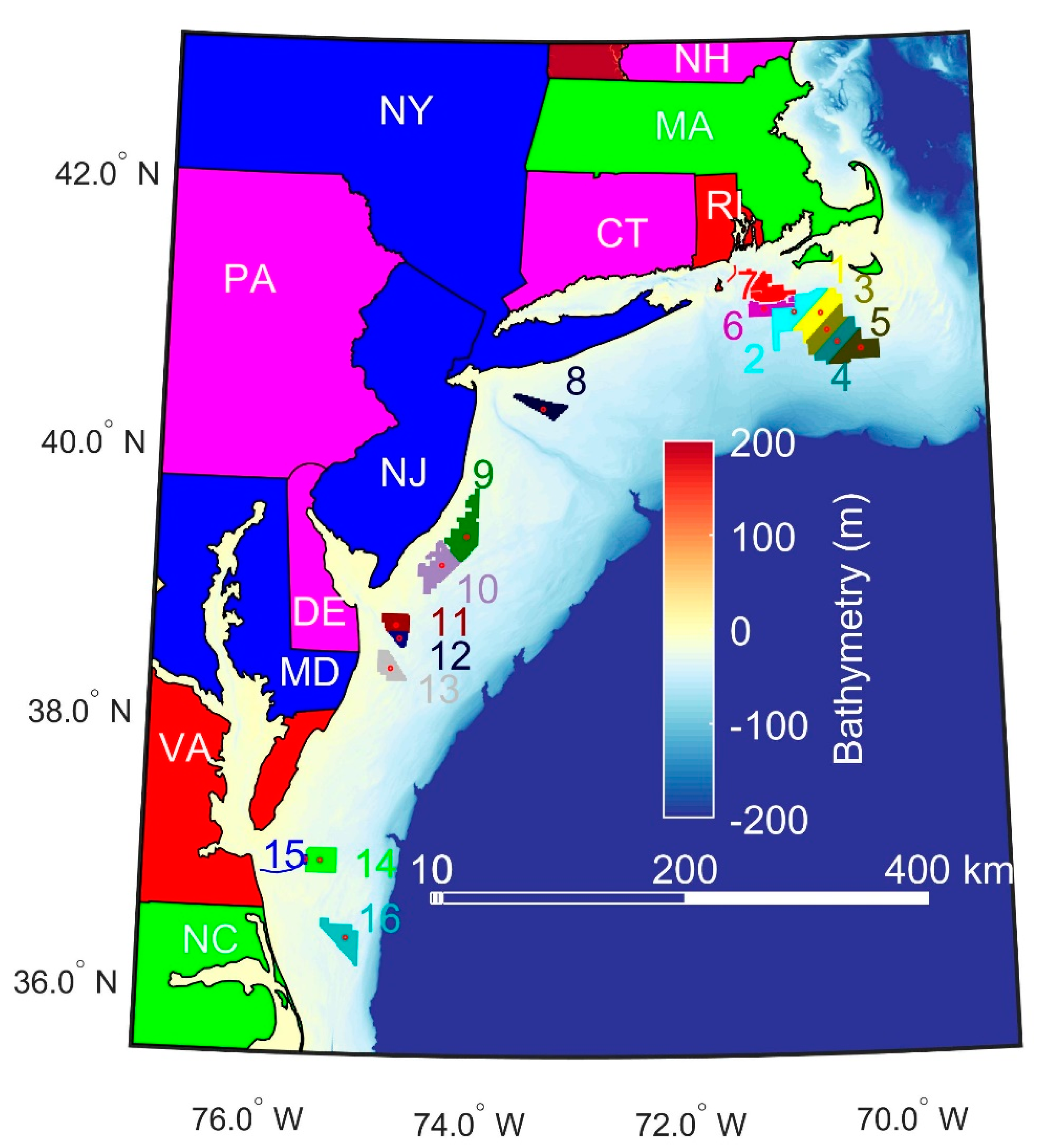
Figure 1. Map of the U.S. eastern seaboard showing bathymetry, states with potential for offshore wind (labelled using the two letter abbreviations given in Table 1 and colored according to the offshore wind energy potential expressed as installed capacity in GW) and locations of the 16 active LA (August 2020). States filled in magenta (CT, DE, NH, PA) have <10 GW offshore wind energy potential, states filled in red (RI, VA) have gross potential of 10–100 GW, states filled in blue (MD, ME, NJ, NY) 100–300 GW and states filled in green (MA, NC) > 300 GW [5]. ME which is north of NH is not shown on the map.
Energies 14 01053 g001
Figure 2. Time series of annual maximum wind speeds for the LA shown in Figure 1. (a) northern group of LA (1–7) off the coast of MA/RI, (b) mid LA 8–13 off the coasts of NY, NJ, DE and MD and (c) south LA 14–16 off the coast of VA and NC. The color coding for the LA is shown in Figure 1.
Energies 14 01053 g002
Figure 3. Mean wind roses for hourly output (1979–2018) at 100 m height from ERA5 for the three groups of LA (see Table 2; NORTH shows LA 1–7, MID shows LA 8–13 and SOUTH shows LA 14–16). The colored areas show the frequency by direction (in 10° bins) of wind speeds in the classes shown in the legend (in ms−1). The frequency (in %) is given below the radial axis (from 0–5%). The magenta symbols show the annual maximum wind speeds (Umax) where the wind speed value is given (in ms−1) above the radial axis (from 20–40 ms−1).
Energies 14 01053 g003
Figure 4. Histograms of the number of annual maximum wind events for each LA cluster by calendar month (a) North (LA 1–7), (c) Mid (LA 8–13), or (e) South (LA 14–16) associated with Tropical Cyclones (TC) (blue), Alberta Clippers (AC) (red), Colorado Lows (CL) (yellow) and ‘other’ (grey). Storm tracks that traversed the northern (b), mid (d) and southern (f) LA and resulted in all of the annual maximum wind speeds are shown in the right-hand panels and the shade of grey used encodes the value of the maximum wind speed in the LA (darkest denoting wind speeds in excess of 33 ms−1). The cyclone origins are designated according to the geographic location in which the cyclone is first identified. The area from which AC originate is defined as 85 to 115° W, 30 to 40° N and is shown in red, the area from which CL originate is defined as 85 to 115° W, 40 to 75° N and is shown in yellow, TC are identified as being any storm that originate south of 30° N. All other cyclones are classed as ‘other’. LA centroids in each group are shown by red dots.
Energies 14 01053 g004
Figure 5. Comparison of U50 for each LA from the different methods (the colored symbols). The open symbol shows the 40-year maximum wind speed U40 from the ERA5 data (Table S1). The error bars show the maximum and minimum wind speed from the 95th confidence interval estimated using boot-strapping for GML and GG/GMM (the latter are offset in the horizontal to aid clarity).
Energies 14 01053 g005
Figure 6. Gumbel-Graphical plots of the ranked annual maximum wind speeds Umax against the reduced Gumbel variate y (see Equations (7)–(9)) for the 16 LA (shown in the upper right on each panel). The color coding is as in Figure 1 and Figure 2. The north LA are shown in the top row, the mid LA in the central row and the south LA in the bottom row. The LA numbers are indicated in the top right of each panel. The coefficient of determination r2 is given for each site at the bottom of each panel.
Energies 14 01053 g006
Figure 7. Histograms of the hourly wind speed data for each LA. The color coding is as in Figure 1 and Figure 2. The north LA are shown in the top row, the mid LA in the central row and the south LA in the bottom row. The LA numbers are indicated in the top right of each panel. The numbers at the bottom of each panel are the Weibull scale parameter (above) and the Weibull shape parameter (below). The red line is the two parameter Weibull fit to the distributions.
Energies 14 01053 g007
Figure 8. Histograms of the annual maximum wind speed data for each LA. The color coding is as in Figure 1 and Figure 2. The north LA are shown in the top row, the mid LA in the central row and the south LA in the bottom row. The LA numbers are indicated in the top right of each panel. The red line indicates the fit to the Gumbel distribution from the maximum likelihood method. The black line shows the 3 parameter GEV fit (Equation (1)).
Energies 14 01053 g008
Figure 9. Time series of annual maximum wave heights Hmax from ERA5 for the LA shown in Figure 1. The top panel shows results for the northern group of LA (1–7) off the coast of MA/RI, the center panel shows the mid LA 8–13 off the coasts of NY, NJ, DE and MD and the lower panel the south LA 14–16 off the coast of VA and NC. The color coding for the individual LA is shown in Figure 1b. Because the ERA5 grid for wave data is at a lower resolution, some of the LA are in the same ERA5 grid (1&3, 6&7, 11,12 & 13, 14&15) hence these data points overlie each other.
Energies 14 01053 g009
Figure 10. The 50-year return period estimates of (a) Hs and (b) Hmax over the 16 LA from the different distribution fitting approaches. Figure (a) also shows water depth at the central location of each LA and Figure (b) shows the GG U50 wind speed for each LA.
Energies 14 01053 g010
Figure 11. The 1-year return period estimates of (a) Hs and (b) Hmax over the 16 LA from the different distribution fitting approaches.
Energies 14 01053 g011
Table 1. Offshore wind energy potential of U.S. east coast states that have offshore wind lease areas (LA); Connecticut, Delaware, Massachusetts, Maryland, Maine, New Hampshire, New Jersey, New York, North Carolina, Pennsylvania, Rhode Island and Virginia.
StateAbbreviationOffshore Wind Gross Potential (GW) [5]Offshore Wind Electricity Generation Potential (TWh/y) [5]2018 Electricity Generation from Wind GWh/year [12]2018 Total Electricity Generation TWh/year [12] Current Electricity from Onshore Wind [6] (% of Total Generation)Potential Contribution to Electricity from Offshore Wind (% of Current Generation)
ConnecticutCT4.61712.239.40.043.1
DelawareDE9.137.95.26.20.1611.3
MaineME127.5645.92284.311.320.25715.9
MarylandMD130.8603.257043.81.31377.2
MassachusettsMA545.82858.122127.20.810507.7
New HampshireNH2.19.40.417.10.055.0
New JerseyNJ165.5796.222.5750.01061.6
New YorkNY165.6786.13998.3132.53.0593.3
North CarolinaNC807.43661.3549.8134.30.42726.2
PennsylvaniaPA5.724.33566.9215.41.711.3
Rhode IslandRI21.3103.1158.68.41.91227.4
VirginiaVI93.3404.5172.895.50.2423.6
Sum of all 12 states 2078.79947.011,562.0806.11.41234.0
US Total 10,799.944,378.2272,667.04178.07.11062.2
Table 2. Offshore LA for wind developments off the U.S. east coast. Data from https://www.boem.gov/renewable-energy/lease-and-grant-information and https://maps.ngdc.noaa.gov/viewers/bathymetry/ and https://oceancolor.gsfc.nasa.gov/docs/distfromcoast/. Centre latitudes and longitudes are estimated from shapefiles available from BOEM [14]. * in second column denote LA that fall within the same ERA5 grid cell for wind speeds (LA 3 and 4). †, ‡, # and ^ in second column denote LA that fall within the same ERA5 grid cell for waves (LA 1 and 3, 6 and 7, 11–13 and 14 and 15, respectively). The final column shows the mean annual mean wind speed computed from the ERA5 hourly output at 100 m height.
Group LA #LesseeStateArea (km2)IdentifierYear IssuedCenter Latitude (N) Center Longitude (W)Water Depth (m)Distance to Coast (km)Mean Annual Mean Wind Speed (ms−1)
North1 †Vineyard WindMA675.7OCS-A 0501201540.96770.58150359.16
2Bay State WindMA759.2OCS-A 0500201540.97870.84251309.12
3 *,†EquinorMA521.5OCS-A 0520201840.83970.5225653 9.17
4 *Mayflower WindMA515.7OCS-A 0521201840.7570.42651619.17
5Vineyard WindMA535.9OCS-A 0522201840.69670.19646659.17
6 ‡Deepwater Wind New EnglandRI/MA272.3OCS-A 0487201341.11971.07537269.02
7 ‡Deepwater Wind New EnglandRI/MA394.7OCS-A 0486201341.00671.13647319.01
Mid8EquinorNY321.3OCS-A 0512201740.27473.31538458.55
9Atlantic Shores Offshore WindNJ742.3OCS-A 0499201639.32174.04624318.55
10Ocean WindNJ649.7OCS-A 0498201639.10674.27924328.54
11 #Garden State Offshore Energy IDE283.8OCS-A 0482201238.65874.70427318.02
12 #SkipjackDE106.6OCS-A 0519201838.56174.67133388.11
13 #US WindMD322.7OCS-A 0490201438.33774.75029288.24
South14 ^Virginia Electric and Power CompanyVA456.7OCS-A 0483201336.90775.36126528.30
15 ^Virginia, Dept Mines, Min. Energy (Research)VA8.6OCS-A 0497201536.91175.49525428.15
16Avangrid RenewablesNC495.6OCS-A 0508201736.34275.10837588.34
Table 3. Method employed here to compute extreme wind speeds.
MethodDescriptionDescriptionReferences
Uref U r e f = 5 U a v e (5)Method used in IEC standards to derive a reference 50-year return period wind speed at hub-height[20]
Gumbel-graphical
(GG)
y G u m b e l = l n ( l n [ m 0.44 N + 0.12 ] ) ( 6 )
U m a x ^ =   β y G u m b e l + μ (7)
Samples of annual maximum wind speed (Umax) are ranked and plotted against the reduced variate yGumbel (where m is the rank order position and N is the total sample size) and are subject to linear fitting using the least squares method to derive the slope and intercept (β and μ). In the absence of a mixed climate for extreme wind speeds [52,53], this relationship is linear. [54]
Gumbel-Weibull
(GW)
F ( U ) = 1 e x p [ ( U c ) k ] (8)
β = 1 / [ k c ( ( l n ( n i n d ) ) 1 1 k ) ] (9)
μ = c ( l n ( n i n d ) ) 1 / k (10)
n i n d = n ( 1 r 1 1 + r 1 )   ( 11 )
Wind speed (U) time series typically fit the two-parameter Weibull distribution [55,56] with scale parameter c and shape parameter k (Equation (8)) derived here using maximum likelihood methods. The resulting Weibull distribution parameters are linked to the Gumbel parameters using Equations (9) and (10). Note: nind is the number of independent observations (i.e., effective sample size approximated here using the lag-1 autocorrelation (r1) as where n’ is the sample size). While this method does not require multiple decades of data to obtain a good fit to the Weibull distribution, the fitting of the tail of the distribution is vulnerable to under-sampling of intense wind speeds.[56]
Gumbel Method of Moments
(GMM)
β = 6 π σ (12)
μ = U ¯ γ β (13)
γ = Euler’s constant (0.577216)
The mean ( U ¯ ) and standard deviation (σ) of the samples of annual maximum wind speed (Umax) are used to derive the Gumbel distribution parameters (μ and β) following Equations (12) and (13). This method is fully analytical and uncertainty for the values of UT calculated using this method can be found using the addition of the third and fourth moments.[57]
Gumbel Maximum Likelihood (GML) Approach is implemented using fitdist in Matlab. Maximum likelihood estimation methods (with iteration) are used to derive μ and β from the samples of annual maximum wind speed (Umax). This is a more computationally demanding but is a non-parametric approach. [58]
Three parameter GEV with MLApproach is implemented using fitdist in Matlab.Maximum likelihood estimation methods (with iteration) are used to derive the 3 parameters in Equation (1) from samples of Umax. [51]
Table 4. One-year return periods for Hmax and Hs (m) for the different LA determined by three different methods. LA that are within a common ERA5 grid cell for wave output are clustered in the same row. Also shown is the co-occurrence of annual maximum Hmax and Umax sampled in three different ways; in the first analysis co-occurrence was specified as the percentage of the 40 years wherein the maximum absolute wave height occurred within 1.5 days of the maximum wind speed (headed; ±1.5 day), or a ±3 h time window of the maximum wind speed (headed; ±3 h), and the percentage of the top 3 events in each year co-occurring within a time window of ±1.5 days of the maximum wind speed (headed; Top 3 ± 1.5 day). Note because of the higher resolution of the wind output the results for two LA may derive a common wave grid cell but different wind grid cells. Hence multiple results are reported for those LA.
LAHsHmaxCo-Occurrence of Maximum Hmax and Umax
Method⇒GGGMMGMLGGGMMGML±1.5 day±3 hTop 3 ± 1.5 day
1&36.265.757.0411.5510.8812.7858,5853,5354,55
26.155.616.9511.4410.7812.85655856
46.856.587.9212.9912.5514.94484553
56.967.327.9713.1612.8514.97403848
6&76.146.216.9511.4410.7112.8665,6560,6054,55
85.905.597.0011.1510.7113.10403844
94.254.074.797.267.048.06484848
105.014.805.649.058.049.92383343
11,12,135.395.276.219.898.8911.2340,48,5333,40,4543,44,49
14&154.304.134.777.577.438.2050,5050,4852,54
165.925.686.8310.8710.6612.27635556
Publisher’s Note: MDPI stays neutral with regard to jurisdictional claims in published maps and institutional affiliations.