Article

Fractal Characterization of Complex Hydraulic Fractures in Oil Shale via Topology

1
College of Architecture and Environment, Sichuan University, Chengdu 610065, China
2
Institute of New Energy and Low-Carbon Technology, Sichuan University, Chengdu 610207, China
3
State Key Laboratory of Shale Oil and Gas Enrichment Mechanisms and Effective Development, Research Institute of Petroleum Exploration and Development of SINOPEC, Beijing 100038, China
*
Author to whom correspondence should be addressed.
Energies 2021, 14(4), 1123; https://doi.org/10.3390/en14041123
Submission received: 30 January 2021 / Revised: 13 February 2021 / Accepted: 18 February 2021 / Published: 20 February 2021
(This article belongs to the Special Issue Oil and Gas Markets: Current Challenges and Future Perspectives)

Abstract

:
The formation of complex fracture networks through the fracturing technology is a crucial operation used to improve the production capacity of tight gas/oil. In this study, physical simulation experiments of hydraulic fracturing were conducted with a true triaxial test system on cubic shale oil samples from the Yanchang Formation, China. The fractures were scanned by CT both before and after the experiments and then reconstructed in 3D. The complexity of fracture networks was investigated quantitatively by the fractal theory with topology. Finally, the effect of the horizontal stress ratio, fluid viscosity, and natural fractures on the complexity of the fracture networks was discussed. The results indicate that the method based on fractal theory and topology can effectively characterize the complexity of the fracture network. The change rates of the fractal dimension (K) are 0.45–3.64%, and the fractal dimensions (DNH) of the 3D fracture network after fracturing are 1.9522–2.1837, the number of connections per branch after fracturing (CB) are 1.57–2.0. The change rate of the fractal dimension and the horizontal stress ratio are negatively correlated. However, the change rate of the fractal dimension first increases and then decreases under increasing fluid viscosities, and a transition occurs at a fluid viscosity of 5.0 mPa·s. Whether under different horizontal stress ratios or fluid viscosities, the complexity of the fracture networks after fracturing can be divided into four levels according to DNH and CB. Complex fracture networks are more easily formed under a lower horizontal stress ratio and a relatively low fluid viscosity. A fracturing fluid viscosity that is too low or too high limits the formation of a fracture network.

Graphical Abstract

1. Introduction

Shale oil is an unconventional petroleum resource and has great potential for exploration and development [1,2]. The global shale oil geological resources add up to 936.835 billion tons, with 61.847 billion tons of technically recoverable resources. In addition, the shale oil reserve in China is abundant, with 4.393 billion tons of technically recoverable resources, ranking third among all the countries worldwide [3]. Due to the ultralow permeability of shale oil reservoirs, hydraulic fracturing is conducted to promote the break the rock and form complex fracture networks, thereby increasing the fracture conductivity and the production of unconventional gas/oil [4,5,6,7].
The conductivity of fracture networks after fracturing can be characterized by the complexity of the fractures [8], and they have a positive correlation. Therefore, the quantitative characterization of the complexity of fracture networks after fracturing can be used to obtain an index of reservoir reconstruction efficiency. Tracers [9,10], split rock samples [11,12], and fluorescent methods [13] are used to characterize fracture networks in the laboratory. However, these methods can damage the rocks, causing secondary cracks to form when these methods are used to characterize a fracture network, and it is difficult to characterize a 3D fracture network with these methods. Acoustic emission [14,15] and CT techniques are nondestructive ways of characterizing fracture networks. Due to the high clay content and abundant natural fractures in shale samples, acoustic emission energy is relatively weak during fracture propagation [16]. Moreover, the acoustic emission results are composed of events, and it is difficult to combine these events to accurately describe a fracture surface [17]. Generally, acoustic emission results can be verified by other methods, such as CT. The main fracture directions predicted via CT scanning have been consistent with the results of acoustic emission monitoring. Thus, the feasibility of acoustic emission has been demonstrated by CT [18,19].
The CT scanning method has been widely used in rock damage experiments [20,21,22]. Some researchers have obtained a relatively high-accuracy spatial geometry of the fractures and porosity in samples via the CT scanning technology [23,24,25]. In research on the initiation, propagation and closure of fractures [26,27,28,29], the morphology and internal structure of fractures have been observed by microscopy and CT scanning. These abovementioned scholars reconstructed only 2D fractures and did not carry out 3D fracture reconstruction and visualization. Two-dimensional fractures reflect only the fracture geometry along a certain plane and cannot truly represent the morphology and distribution of fractures in space. Some scholars [30,31] reconstructed and visualized 3D fractures in different rock types. Jiang et al. [32] and Liu et al. [33] investigated the effects of in situ stress and fracturing fluid on the propagation and distribution characteristics of hydraulic fractures based on the 3D reconstruction technology. Even though the 3D reconstruction of fracture networks was carried out in these studies, reconstruction has been performed mainly qualitatively. The quantitative characterization of fracture complexity can accurately describe reservoir reconstruction efficiency [34]. Therefore, we need to introduce a quantitative characterization method to investigate the 3D fracture network complexity.
In previous studies, there are many ways to characterize the complexity of fractures, such as fracture density [35], topology [36], anisotropic parameters based on wave velocity [37], and fractal dimensions [38]. Among them, the fractal theory can quantitatively describe the distribution characteristics of fractures under the same fracture density. Williams et al. [39,40] described the fractal characteristics of porous media and the fractal phenomenon in the process of porous media transmission. Sahimi et al. [41,42] believed that the fractal theory is a very effective method for calculating complex fracture networks. Chilingarian [43] used a statistically significant self-similar fractal method to calculate the fractal dimension of natural fracture distribution. Some domestic scholars have also carried out many meaningful studies based on fractal reservoirs. In China, Xie [44] systematically applied the fractal theory to the rock field. Many scholars [45,46,47,48] have begun to study the fractal characteristics of rock pore structures obtained from mercury penetration, CT, and low-pressure N2 adsorption. Simultaneously, the fractal theory has been used to characterize fracture networks. Based on SEM results, Li et al. [49] evaluated the relationship between fractal dimension, rock composition, and stress state. Based on CT scanning, some scholars [50,51,52] characterized the fracture networks of coal rocks by the fractal theory and discussed the effect of loading on its evolution. Zhao et al. [53] found that the trend of the strength parameter decreased with the increase in the fractal dimension of reconstructed fractures. Liu et al. [54] characterized the growth and distribution patterns of fractures in media by combining the fractal theory and CT images.
However, the fractal dimension cannot describe the connectivity of fracture networks. Topology is an area of mathematics that deals with the abstraction and generalization of spatial relationships such as connectivity and continuity [55,56,57]. A description of the fracture network connection can be conducted by means of topology to avoid the defects of fractal theory [36]. Since topology cannot characterize the distribution and quantity number of fractures, it is also inaccurate to describe the complexity of fracture networks using only topology. Therefore, it is necessary to consider both fractal dimension and topology to characterize the complexity of fracture networks. In this study, the 3D fractal characterization of a complex fracture network after the hydraulic fracturing of an oil shale was investigated based on topology.
In this study, we quantitatively characterized the complexity of fracture networks before and after hydraulic fracturing by the fractal theory and topology. To investigate the effect of the horizontal stress ratio, fluid viscosity, and natural fractures on the complexity of fracture networks in oil shale, hydraulic fracturing physical simulation experiments and 3D fracture reconstruction were carried out. We focused on discussing the fractal dimension change rate (K) and the number of connections per fracture branch (CB) before and after fracturing under different horizontal stress ratios and fluid viscosities.

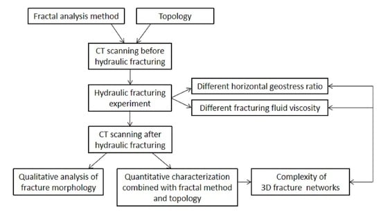
2. Materials and Methods

2.1. Sample Preparation

Shale oil samples were taken from the Triassic Yanchang formation in Tongchuan city, Shaanxi Province, China. Chang 7 covers an area of approximately 100 × 103 km2, with a burial depth range from 600 to 2900 m and thickness range from 70 to 130 m [58]. The shale outcrop is shown in Figure 1a. The XRD (X-ray diffraction) test results of shale rock samples are shown in Table 1, which illustrate the mineral composition of oil shale. The collected Chang 7 shale has a tensile strength of 4.76 MPa, a Young’s modulus of 3.61 GPa, and a Poisson ratio of 0.3336. The collected shale was processed into standard 100 × 100 × 100 mm cubic samples by cutting, core drilling, and grinding to ensure that the opposite faces were parallel. A simulated wellbore with a depth of 50 mm and a diameter of 12 mm was drilled in the center of each sample. A high-strength steel pipe with a length of 50 mm, an outer diameter of 8 mm, and an inner diameter of 4 mm was used to simulate the sleeve. Then, the wellbore was sealed by a high-strength adhesive glue, as shown in Figure 1b.

2.2. Experimental Scheme

The shale hydraulic fracturing experiments were mainly performed to consider the influence of the horizontal stress ratio and fluid viscosity on the complexity and morphology of the fracture networks after shale fracturing. The wellbore direction was designed to be perpendicular to the bedding planes. According to the in situ stress data in the Triassic Yanchang Formation, Ordos Basin, the maximum vertical principal stress σ 1 is approximately 40 MPa, and the maximum horizontal principal stress σ 2 and minimum principal stress σ 3 are 25.8–31.5 MPa and 22.5–25.8 MPa, respectively. The specific experimental parameters are shown in Table 2. In addition, tests H1 to H4 were conducted to investigate the effect of different horizontal stress conditions on the resulting fracture networks under a fluid viscosity of 17.1 mPa·s. Tests F1 to F4, and H2 were conducted to investigate the effect of different fluid viscosity conditions on the resulting fracture networks under a horizontal stress ratio of 1.353. The hydraulic fracturing liquid is a solution of guar gum and clear water.

2.3. Experimental Apparatus and Procedure

The large-scale true triaxial physical model test system was used to carry out hydraulic fracturing simulation experiments. The industrial CT, in the Key Laboratory of Deep Underground Science and Engineering (Sichuan University), Ministry of Education, was used to characterize the fracture networks before and after fracturing. A scanning voltage of 250 kV and a scanning current of 200 μA were selected to ensure that the resolution was less than 80 μm. For each sample, the experimental procedures were as follows:
  • All the samples were scanned before fracturing so that the further development of the natural fractures could be discussed.
  • After sealing the wellbore, a sample was placed in the true triaxial hydraulic fracturing experimental apparatus. To avoid damage to the samples as the confining pressure was applied, the stresses in the three directions are first loaded to σ 3 , two are then further loaded to σ 2 , and one is finally further loaded to σ 1 .
  • Before fracturing, a pressure of 0.5 MPa was applied to the wellbore to check whether the sealed sample would leak. A hydraulic pump was used to load the sample to failure with a flow rate of 0.06 mL/s.
  • The shale samples were also scanned after fracturing, and the 3D fracture networks were reconstructed to study the complexity of the fracture network.

2.4. Reconstruction of 3D Fractures

The 3D morphology of each fracture network was reconstructed by means of the software Mimics (http://biomedical.materialise.com/mimics (accessed on 17 February 2021), Materialise company, Belgium) based on a set of 2D images. To accurately extract the fractures, it was necessary to identify the threshold value of the shale components. The fracture, shale matrix, and mineral composition can be represented by different gray values in the CT images [32].
A section line was used to determine the threshold value of the fractures, shale matrix, and high-density minerals. Natural fractures, hydraulic fractures, and high-density minerals were observed along the section line, as shown in Figure 2a. The corresponding gray value curve clearly shows two peaks and two troughs in Figure 2b. High-density minerals have large gray values, while the gray values of fractures are relatively small. Moreover, the amplitude of the gray values of the natural fractures were significantly larger than those of the hydraulic fractures, which also indicates that natural fractures are easier to observe. The larger the fracture is, the smaller the corresponding gray values. Based on this principle, the fractures observed in the CT slices scanned before and after fracturing can be segmented, and then 3D fracture networks can be reconstructed according to the regional growth, morphological expansion, and corrosion technology.
Figure 3 depicts the 3D reconstructed fractures of sample H3 and shows a picture of the sample taken after the hydraulic fracturing experiment. In the reconstructed model, the natural fractures are represented by red, the hydraulic fractures are represented by blue, and the wellbore is represented by white. The 3D reconstructed fractures closely match the fractures on the surface of the samples, and the fractures that cannot be observed on the surface of the samples are reflected in the reconstructed model. The reconstruction results can be used to visually observe the morphology of natural fractures and hydraulic fractures inside the shale sample.

3. Experimental Results and Discussion

3.1. Fractal Method and Network Topology

3.1.1. Fractal Calculation Method

For digital images of 3D fractures, the fractal dimension can be calculated by the cubic covering method [47]. The digital image of a 3D fracture (Figure 4a) consists of a series of pixels in sequence. Each pixel has a corresponding color, and a 3D digital image of size m × n × h pixels can be regarded as a matrix of size m × n × h. The space is divided into cubes of different sizes (Figure 4b).
Through image preprocessing and binarization, a 3D fracture image is obtained. The voxel value is 0 or 1, respectively, and the value of 1 represents the fracture. The entire 3D fracture space is traversed to obtain the total number of cubes Nk under different cube lengths δk. For each value of δk, the corresponding Nk can be calculated, and a series of data pairs (δk, Nk) can be obtained. Equation (1) can be obtained by linearly fitting the data points (lnNk, lnδk ) in the scale-independent region by the method of least squares, and the slope is the fractal dimension D of the 3D fracture:
ln N k = D ( ln δ k ) + b

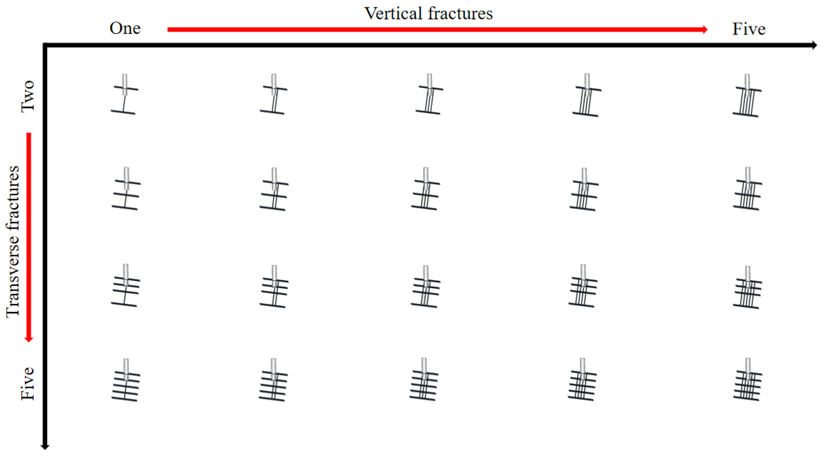
3.1.2. Network Topology

In the two-dimensional fracture network, the fracture is composed of a series of lines, nodes, and branches. Each fracture in the plane has its own fracture trace and two terminal nodes. In addition, if the fracture crosses other fractures, there will be more nodes. According to the research of Manzocchi [59], three types of nodes (I-nodes; X-nodes; Y-nodes) can be recognized, as shown in Figure 5a. In the 3D space, any fracture system will consist of a number of finite planes, and also contain three types of nodes, as shown in Figure 5b.
The number of different node types can be used to calculate the average number of connection points of the branch, a topological parameter that can characterize the connectivity of the fracture network. Each branch will have two nodes, with an I-node contributing to one branch, a Y-node to three branches and an X-node to four branches [36]. Hence, we can derive the number of branches (NB) where:
N B = 1 2 ( N I + 3 N Y + 4 N X )
X-nodes and Y-nodes are the connection points of branches. Each Y-node belongs to three branches, and each X-node belongs to four branches, since an average number of connections per branch (CB) can be derived, where:
C B = ( 3 N Y + 4 N X ) / N B
C B = ( 6 N Y + 8 N X ) / ( N I + 3 N Y + 4 N X )
According to Equation (4), when the fracture network is dominated by I-nodes, the value of CB tends to 0. When the fracture network is dominated by Y-nodes and X-nodes, the value of CB tends to 2, and the corresponding fracture network has greater connectivity.

3.1.3. Fractal Character and Topology of Typical Fractures

In the characterized reconstruction effect of fracture networks after hydraulic fracturing, the connectivity of fractures must be considered. To illustrate that the fractal dimension cannot accurately characterize the complexity of fracture networks, the connectivity calculation of multiple fracture plane combination models (Figure 6) is carried out. Figure 7 is the relationship between the fractal dimensions (D) and average number of connections per branch (CB) of different fracture plane combination models.
According to Figure 7, models A and B have almost the same fractal dimension, and the distribution of fracture networks is also pretty similar. However, the CB value of model B is greater than that of model A, which means that model B has better connectivity. Therefore, when the fracture networks have the same fractal dimensions, it is necessary to utilize the connectivity to comprehensively evaluate the complexity of fracture networks.

3.1.4. Fractal Character and Topology of Fracture Network after Fracturing

Based on the fractal method, the fractal dimension of the fractures in the samples before and after the hydraulic fracturing experiments can be calculated for different horizontal stress ratios and different fluid viscosities. The calculation results of the fractal dimensions of all the 3D reconstructed fractures before and after the hydraulic fracturing experiments are shown in Figure 8. The change rate K of the fractal dimension of the fractures in a sample before and after the fracturing experiment is defined by the following Equation (5).
K = ( D N H D N ) / D N × 100 %
where DN is the fractal dimension before the fracturing experiment and DNH is the fractal dimension after the fracturing experiment.
Table 3 shows the fractal dimensions of 3D reconstructed fractures before and after fracturing, and the number of connections per branch of each fracture network after fracturing. The fractal dimensions of the final 3D fracture network after the fracturing experiments (DNH) are 1.9522–2.1837. However, the fractal dimensions of just the natural fractures (DN) are 1.9434–2.1473, which are smaller than the fractal dimensions of the corresponding final fracture networks after the fracturing experiments. The change rate of the fractal dimension (K) is 0.45%–3.64%, indicating that the complexity of the fracture network increased due to fracturing. The number of connections per branch (CB) are 1.57–2.0, which indicates that the fracture networks have a different connectivity after fracturing. When both K and CB are maximum, the reconstruction efficiency of the fracture network after fracturing is the best. However, it is generally impossible that both of them achieve the maximum value at the same time.

3.2. Effect of the Horizontal Stress Ratio on the Complexity of Fracture Networks

Samples H1, H2, H3, and H4 were tested at horizontal stress ratios of 1.000, 1.353, 1.529, and 1.647, and the fractal dimensions of the fracture networks after fracturing were 2.1194, 2.1289, 2.0326, and 1.9522. In addition, the number of connections per branch after fracturing were 1.68, 1.57, 2.00, and 1.85, respectively. Figure 9 shows the fractal dimensions of the fracture networks and the change rate of the fractal dimensions at different horizontal stress ratios before and after fracturing. The change rate of the fractal dimension ranges from 0.45% to 2.58% under different horizontal stress ratios. There is always a negative correlation between the fractal dimension change rate and the horizontal stress ratio. For a horizontal stress ratio less than 1.529, the change rate of the fractal dimension decreases slowly with the increase in the horizontal stress ratio. Once the horizontal stress ratio exceeds 1.529, the rate of change in the fractal dimension decreases sharply. This result implies that when the horizontal stress ratio increases, the growth and complexity of the fracture network gradually decreases.
Figure 10 shows the distribution of fractal dimension (DNH) and the number of connections per branch (CB) of fractures under different horizontal stress ratios after fracturing. DNH is 1.9522–2.1289 and CB is 1.57–2.00, and fracture networks after fracturing have different complexities which can be divided into four levels. The samples with a fracture network complexity in the first to fourth levels are respectively H1, H2, H3, and H4, and the fracture network at the first level is the most complex. When a fracture network has both relatively large DNH and CB, that is, its coordinates are located in the upper right corner of the coordinate axis, the fracture network is more complicated. Therefore, the complexity of the fracture network of samples H1 and H2 is greater than that of sample H3. In addition, DNH and CB of the fracture network of sample H3 are larger compared with that of sample H4, which means that the complexity of the fracture network of samples H3 is greater. The results show that it is more conducive to the formation of complex fracture networks at a low horizontal stress ratio.
When the horizontal stress ratio is 1.000, the change rate of the fractal dimension is the largest, which means that the fractures formed during the fracturing experiment are the most developed. For a lower horizontal stress ratio, deflection easily occurs, so the fracturing fluid tends to permeate and propagate along the natural fractures to form complex hydraulic fractures, as in shown Figure 8a. The fracture network complexity of sample H1 after fracturing is at the first level, and has a large DNH and a small CB (Figure 10). Under this condition, the number of fractures are the most, the connectivity of fractures is relatively good, and the fracture network is the most complicated.
For the horizontal stress ratio of 1.353, compared to the results for a horizontal stress ratio of 1.000, the change rate of the fractal dimension is smaller, and the complexity of the fractures formed during the fracturing experiment is reduced. Natural microfractures also exist in the location where the hydraulic fracture develops in sample H2, which promotes the formation of a single fracture. The formation of a single hydraulic fracture in Figure 8b is beneficial in terms of the communication with the natural fractures to form a complex fracture morphology. However, apart from the formation of the main hydraulic fracture, there are no additional fractures that extend along the natural fractures and bedding planes. The fracture network complexity of sample H2 after fracturing is at the second level, and has the largest DNH and smallest CB. At this time, there are many fractures, the connectivity of fractures is the worst, and the fracture network is relatively complicated.
When the horizontal stress ratio increases to 1.529, the change rate of the fractal dimension also decreases. The fracture network complexity of sample H3 after fracturing is at the third level, and has the relatively small DNH and largest CB. There are relatively more fractures, the best fracture connectivity, and the simple fracture network at this horizontal stress ratio. When the horizontal stress ratio increased to 1.647, hydraulic fractures were less likely to form and extend in sample H4 during the fracturing experiment. The fracture network complexity of sample H4 after fracturing is at the fourth level, and has the smallest DNH and a large CB. In addition, there are relatively few fractures, excellent fracture connectivity, and the simplest fracture network.

3.3. Effect of Fluid Viscosity on the Fractal Dimension and Complexity of Fracture Networks

Samples F1, F2, F3, H2, and F4 were tested at fluid viscosities of 1.3, 3.2, 5.0, 17.1, and 31.6 mPa·s, and the fractal dimensions of fracture networks after fracturing were 2.1795, 2.1837, 2.1271, 2.1289, and 2.0810. In addition, the number of connections per branch after fracturing were 1.70, 1.72, 1.81, 1.57, and 1.62, respectively. Figure 11 shows the relationship between the fractal dimension, the change rate of the fractal dimension, and the fluid viscosity. The change rate of the fractal dimension varies from 1.50% to 3.64% under the different fluid viscosities tested. There is a transition in the change rate of the fractal dimension of the fracture networks before and after fracturing. The fluid viscosity of 5.0 mPa·s separates the change rate of the fractal dimension into two parts. The change rate of the fractal dimension at the fluid viscosity of 5.0 mPa·s is the maximum value. For a fluid viscosity less than 5.0 mPa·s, the change rate of the fractal dimension increases with the fluid viscosity. However, when the fluid viscosity is over 5.0 mPa·s and less than 17.1 mPa·s, the rate of change in the fractal dimension slowly decreases. In addition, due to the differences in the natural fracture distribution, the change rate of the fractal dimension at the fluid viscosity of 31.6 mPa·s is greater than that at the fluid viscosity of 17.1 mPa·s. The results show that a fracturing fluid with a low viscosity is favorable for the generation of an effective fracture network, but a fracturing fluid viscosity that is too low or too high will limit the formation of a fracture network.
The distribution of fractal dimension (DNH) under different fluid viscosities is 2.0810~2.1837, and the number of connections per branch (CB) is from 1.57 to 1.81, as shown in Figure 12. Similarly, the complexities of fracture networks after fracturing can be divided into four levels. The samples with the first level of fracture network complexity are F1 and F2, the second to fourth levels are respectively F3, H2, and F4. Compared with sample F1, sample F2 has both larger DNH and CB, which indicates that the fracture network of sample F2 is more developed after fracturing. It also shows that that too low fluid viscosity (1.3 mPa·s) is not conducive to complex fracture network formation. The fracture networks of samples F3 and H2 have roughly the same fractal dimensions, but the CB of the fracture network of F3 is significantly larger than that of H2. Therefore, compared with sample H2, the fracture morphology of sample F2 is more complicated. By the similar method, it is easy to get that the fracture network of F3 is more than that of F4. The results show that the high viscosity fluid is not conducive to the formation of complex fracture networks.
The change rate of the fractal dimension at the viscosity of 1.3 mPa·s is smaller than that at a viscosity of 3.2 mPa·s, which implies that too low of a viscosity prevents the formation of a larger fracture network. The influence of the flow rate and viscosity of the fracturing fluid on the morphology of hydraulic fractures can be expressed as the product of the parameter q·u, whose unit is N·m [24]. Therefore, too low of a fracturing fluid viscosity, considering the same flow rate, leads to a pressure rate which is insufficient to induce the propagation of hydraulic fractures. Similarly, the change rate of the fractal dimension at a viscosity of 3.2 mPa·s is smaller than that at a viscosity of 5.0 mPa·s. After fracturing, the fracture network complexity of samples F1 and F2 is at the first level, with extremely large DNH and CB. These two samples have the most fractures, excellent fractures connectivity, and the most developed fracture network.
When the fluid viscosity increases from 5.0 to 17.1 mPa·s, the fractal dimension and the change rate of the fractal dimension both decrease gradually. The high-viscosity fracturing fluid reduces the propagation of fractures and induces the formation of a single hydraulic fracture (Figure 8g). The low-viscosity fracturing fluid can increase the fluid loss to these fractures and expand the fluid flow channel. Simultaneously, the low-viscosity fracturing fluid more easily enters the natural fractures and bedding planes, promoting the formation of more complex fracture networks. The fracture network complexity of sample F3 after fracturing is at the second level, with extremely large DNH and CB. There are many fractures in sample F3, the best fracture connectivity and the relatively complicated fracture network.
When the fluid viscosity increases to 17.1 mPa·s, the change rate of the fractal dimension decreases to the lowest. The fracture network complexity of sample H2 is at the third level, with larger DNH and smallest CB. In addition, the sample has many fractures, which are the worst fracture connectivity and relatively simple fracture network.
The natural fracture distribution of sample F4 is concentrated at the bottom of the sample, and the hydraulic fractures extend from the top to the bottom, which leads to a large variation in fractal dimension, as shown in Figure 8h. Therefore, the change rate of the fractal dimension with a viscosity of 31.6 mPa·s is greater than that with a viscosity of 17.1 mPa·s. The fracture network complexity of sample F4 after fracturing is at the fourth level, and has the smallest DNH and relatively small CB. At this time, these are the least fractures with a relatively good fracture connectivity, and the fracture network is the simplest.

4. Conclusions

Based on true triaxial hydraulic fracturing experiments and 3D reconstruction/visualization techniques, this study quantitatively investigates the complexity of fracture networks before and after hydraulic fracturing in shale. The influences of the horizontal stress ratio, fluid viscosity, and natural fractures on the fracture morphology and propagation are also discussed. The following conclusions are drawn:
  • According to the results of fracture plane combination models, the fractal dimension cannot accurately characterize the complexity of fracture networks. The method based on the fractal theory and topology can more effectively characterize the complexity of the fracture network.
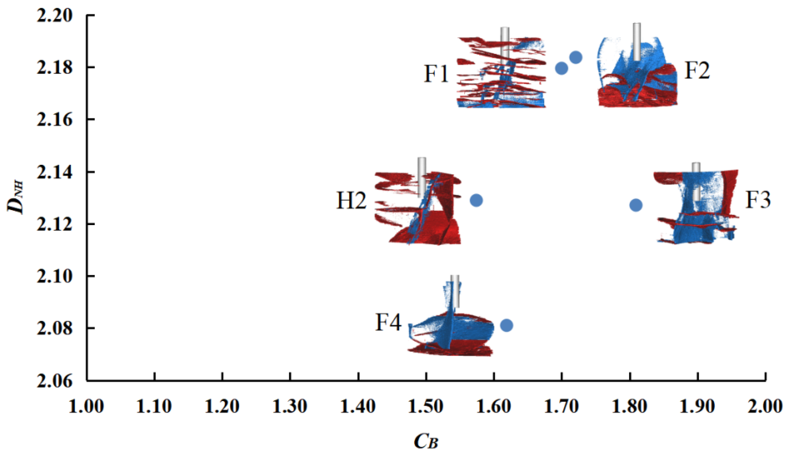
  • Different horizontal stress ratios change the fractal dimension of the fracture network at a rate of 0.45–2.58%, in which a greater horizontal stress ratio tends to correspond to a lower change rate, and vice versa. Under different horizontal stress ratios, DNH is 1.9522–2.1289 and CB is 1.57–2.00, and the complexities of fracture networks after fracturing can be divided into four levels. The result shows that complex fracture networks are more easily formed under a lower horizontal stress ratio.
  • Under different fluid viscosities, the fractal dimensions of fracture networks have a change rate of 1.50–3.64%, where a transition emerges at the fluid viscosity of 5.0 mPa·s. After fracturing, DNH is 2.0810–2.1837 and CB is 1.57 to 1.81. Similarly, the complexities of fracture networks after fracturing can be divided into four levels. A complex fracture network tends to be stimulated under the conditions of a low fluid viscosity: The fluid viscosity must not be too low or too high.

Author Contributions

In this study, Q.H. is in charge of the research of formal analysis and writing; B.H. carried out the works of conceptualization and formal analysis; F.L. provided funding for the research; A.S. participated in project administration; J.C. provided research resources; L.X. supevised the whole research; W.N. is in charge of the works of Investigation. All authors have read and agreed to the published version of the manuscript.

Funding

This research was funded by the National Natural Science Foundation of China [no. 11872258] and the Department of Science and Technology of Sichuan Province [no. 2019YFH0121].

Conflicts of Interest

The authors declare no conflict of interest.

References

  1. Liu, J.; Xie, L.; Yao, Y.; Gan, Q.; Zhao, P.; Du, L. Preliminary Study of Influence Factors and Estimation Model of the Enhanced Gas Recovery Stimulated by Carbon Dioxide Utilization in Shale. ACS Sustain. Chem. Eng. 2019, 7, 20114–20125. [Google Scholar] [CrossRef]
  2. Zhao, W.; Hu, S.; Hou, L.; Yang, T.; Li, X.; Guo, B.; Yang, Z. Types and resource potential of continental shale oil in China and its boundary with tight oil. Pet. Explor. Dev. 2020, 47, 1–11. [Google Scholar] [CrossRef]
  3. Advanced Resources International, Inc. EIA/ARI World Shale Gas and Shale Oil Resource Assessment; Advanced Resources International, Inc.: Arlington, MA, USA, 2013. [Google Scholar]
  4. Java Javadpour, F.; McClure, M.; Naraghi, M. Slip-corrected liquid permeability and its effect on hydraulic fracturing and fluid loss in shale. Fuel 2015, 160, 549–559. [Google Scholar] [CrossRef]
  5. Zhou, T.; Zhang, S.; Yang, L.; Ma, X.; Zou, Y.; Lin, H. Experimental investigation on fracture surface strength softening induced by fracturing fluid imbibition and its impacts on flow conductivity in shale reservoirs. J. Nat. Gas Sci. Eng. 2016, 36, 893–905. [Google Scholar] [CrossRef]
  6. Liu, J.; Xie, L.; Elsworth, D.; Gan, Q. CO2/CH4 Competitive Adsorption in Shale: Implications for Enhancement in Gas Production and Reduction in Carbon Emissions. Environ. Sci. Technol. 2019, 53, 9328–9336. [Google Scholar] [CrossRef]
  7. Liu, L.; Zhu, W.; Wei, C.; Elsworth, D.; Wang, J. Microcrack-based geomechanical modeling of rock-gas interaction during supercritical CO2 fracturing. J. Pet. Sci. Eng. 2018, 164, 91–102. [Google Scholar] [CrossRef]
  8. Zu Zuloaga-Molero, P.; Yu, W.; Xu, Y.; Sepehrnoori, K.; Li, B. Simulation Study of CO2-EOR in Tight Oil Reservoirs with Complex Fracture Geometries. Sci. Rep. 2016, 6, 33445. [Google Scholar] [CrossRef]
  9. Zhou, J.; Jin, Y.; Chen, M. Experimental investigation of hydraulic fracturing in random naturally fractured blocks. Int. J. Rock Mech. Min. Sci. 2010, 47, 1193–1199. [Google Scholar] [CrossRef]
  10. Zhou, J.; Chen, M.; Jin, Y.; Zhang, G.-Q. Analysis of fracture propagation behavior and fracture geometry using a tri-axial fracturing system in naturally fractured reservoirs. Int. J. Rock Mech. Min. Sci. 2008, 45, 1143–1152. [Google Scholar] [CrossRef]
  11. Yao, F.; Chen, M.; Wu, X.D.; Zhang, G. Physical simulation of hydraulic fracture propagation in naturally fractured formations. Oil Drill. Prod. Technol. 2008, 30, 83–86. [Google Scholar] [CrossRef] [Green Version]
  12. Meng, Q.M.; Zhang, S.C.; Guo, X.M.; Chen, X.H.; Zhang, Y. A primary investigation on propagation mechanism for hydraulic fracture in glutenite formation. J. Oil Gas Technol. 2010, 32, 119–123. [Google Scholar]
  13. Chen, Y.; Nagaya, Y.; Ishida, T. Observations of Fractures Induced by Hydraulic Fracturing in Anisotropic Granite. Rock Mech. Rock Eng. 2015, 48, 1455–1461. [Google Scholar] [CrossRef]
  14. Maxwell, S.C.; Urbancic, T.I.; Steinsberger, N.; Zinno, R. Microseismic imaging of hydraulic fracture complexity in the Barnett Shale. In Proceedings of the Spe Technical Conference & Exhibition, San Antonio, TX, USA, 29 September–2 October 2002. [Google Scholar]
  15. Bunger, A.P.; Kear, J.; Dyskin, A.V.; Pasternak, E. Sustained acoustic emissions following tensile crack propagation in a crystalline rock. Int. J. Fract. 2015, 193, 87–98. [Google Scholar] [CrossRef]
  16. Chen, L.-H.; Chen, W.-C.; Chen, Y.-C.; Benyamin, L.; Li, A.-J. Investigation of Hydraulic Fracture Propagation Using a Post-Peak Control System Coupled with Acoustic Emission. Rock Mech. Rock Eng. 2014, 48, 1233–1248. [Google Scholar] [CrossRef]
  17. Li, D.; Kuang, K.S.C.; Koh, C.G. Fatigue crack sizing in rail steel using crack closure-induced acoustic emission waves. Meas. Sci. Technol. 2017, 28, 065601. [Google Scholar] [CrossRef]
  18. Heng, S.; Yang, C.H.; Zeng, Y.J.; Guo, Y.T.; Hou, Z.K. Experimental study on hydraulic fracture geometry of shale. Chin. J. Geotech. Eng. 2014, 36, 1243–1251. [Google Scholar] [CrossRef]
  19. Ma, X.; Li, N.; Yin, C.; Li, Y.; Zou, Y.; Wu, S.; He, F.; Wang, X.; Zhou, T. Hydraulic fracture propagation geometry and acoustic emission interpretation: A case study of Silurian Longmaxi Formation shale in Sichuan Basin, SW China. Pet. Explor. Dev. 2017, 44, 1030–1037. [Google Scholar] [CrossRef]
  20. Zhang, S.C.; Gou, T.K.; Zhou, T.; Zou, Y.S.; Mu, S. Fracture propagation mechanism experiment of hydraulic fracturing in natural shale. Acta Pet. Sin. 2014, 35, 496–503. [Google Scholar] [CrossRef]
  21. Bohloli, B.; De Pater, C. Experimental study on hydraulic fracturing of soft rocks: Influence of fluid rheology and confining stress. J. Pet. Sci. Eng. 2006, 53, 1–12. [Google Scholar] [CrossRef]
  22. Dong, Y.; Pater, C.J. Observation and modeling of the hydraulic fracture tip in sand. In Proceedings of the 42nd US Rock Mechanics Symposium (USRMS), San Francisco, CA, USA, 29 June–2 July 2008. [Google Scholar]
  23. Sun, Z.Y.; Huang, Z.W.; Liu, C.Y.; Wu, C. Experimental research on hydraulic fracture initiation and propagation by CT scanning. In Proceedings of the Field Exploration & Development Conference, Chengdu, China, 23–25 September 2020. [Google Scholar]
  24. Guo, T.; Zhang, S.; Qu, Z.; Zhou, T.; Xiao, Y.; Gao, J. Experimental study of hydraulic fracturing for shale by stimulated reservoir volume. Fuel 2014, 128, 373–380. [Google Scholar] [CrossRef]
  25. Karpyn, Z.; Alajmi, A.; Radaelli, F.; Halleck, P.; Grader, A. X-ray CT and hydraulic evidence for a relationship between fracture conductivity and adjacent matrix porosity. Eng. Geol. 2009, 103, 139–145. [Google Scholar] [CrossRef]
  26. Zhang, X.; Lu, Y.; Tang, J.; Zhou, Z.; Liao, Y. Experimental study on fracture initiation and propagation in shale using supercritical carbon dioxide fracturing. Fuel 2017, 190, 370–378. [Google Scholar] [CrossRef]
  27. He, J.; Lin, C.; Li, X.; Zhang, Y.; Chen, Y. Initiation, propagation, closure and morphology of hydraulic fractures in sandstone cores. Fuel 2017, 208, 65–70. [Google Scholar] [CrossRef]
  28. Li, Z.; Jia, C.; Yang, C.; Zeng, Y.; ShuaI, H.; Wang, L.; Hou, Z. Propagation of hydraulic fissures and bedding planes in hydraulic fracturing of shale. Chin. J. Rock. Mech. Eng. 2015, 34, 12–20. [Google Scholar] [CrossRef]
  29. Mohmadi, M.; Wan, R.G. Strength and post-peak response of Colorado shale at high pressure and temperature. Int. J. Rock Mech. Min. Sci. 2016, 84, 34–46. [Google Scholar] [CrossRef]
  30. Jia, L.; Chen, M.; Sun, L.; Sun, Z.; Zhang, W.; Zhu, Q.; Sun, Z.; Jin, Y. Experimental study on propagation of hydraulic fracture in volcanic rocks using industrial CT technology. Pet. Explor. Dev. 2013, 40, 405–408. [Google Scholar] [CrossRef]
  31. Raynaud, S.; Fabre, D.; Mazerolle, F.; Geraud, Y.; Latiere, H. Analysis of the internal structure of rocks and characterization of mechanical deformation by a non-destructive method: X-ray tomodensitometry. Tectonophysics 1989, 159, 149–159. [Google Scholar] [CrossRef]
  32. Jiang, C.; Niu, B.; Yin, G.; Zhang, D.; Yu, T.; Wang, P. CT-based 3D reconstruction of the geometry and propagation of hydraulic fracturing in shale. J. Pet. Sci. Eng. 2019, 179, 899–911. [Google Scholar] [CrossRef]
  33. Liu, P.; Ju, Y.; Gao, F.; Ranjith, P.G.; Zhang, Q. CT Identification and Fractal Characterization of 3-D Propagation and Distribution of Hydrofracturing Cracks in Low-Permeability Heterogeneous Rocks. J. Geophys. Res. Solid Earth 2018, 123, 2156–2173. [Google Scholar] [CrossRef]
  34. Zhao, X.; Rui, Z.; Liao, X.; Zhang, R. The qualitative and quantitative fracture evaluation methodology in shale gas reservoir. J. Nat. Gas Sci. Eng. 2015, 27, 486–495. [Google Scholar] [CrossRef]
  35. Tang, C. Progress in Fracture Characterization and Prediction. Sci. Technol. Rev. 2013, 31, 74–79. [Google Scholar]
  36. Sanderson, D.J.; Nixon, C.W. The use of topology in fracture network characterization. J. Struct. Geol. 2015, 72, 55–66. [Google Scholar] [CrossRef]
  37. Cardona, R.; Jenner, E.; Davis, T.L. Fracture network characterization from P- and S-wave data at Weyburn field, Canada. SEG Tech. Program. Expand. Abstr. 2003, 2003, 370–373. [Google Scholar]
  38. Feng, J.; Yu, J.Y. Determination fractal dimension of soil macropore using computed Tomography. J. Irrig. Drain. 2005, 24, 26–28. [Google Scholar]
  39. Williams, J.K.; Dawe, R.A. Fractals? An overview of potential applications to transport in porous media. Transp. Porous Media 1986, 1, 201–209. [Google Scholar] [CrossRef]
  40. Adle, P.M. Transport Processes in Porous Media; Springer: Dordrecht, The Netherlands, 1993. [Google Scholar]
  41. Sahimi, M.; Yortsos, Y.C. Applications of fractal geometry to porous media: A review. Fluid Dyn. 1992, 27, 824–833. [Google Scholar]
  42. Sahimi, M. Flow phenomena in rocks: From continuum models to fractals, percolation, cellular automata, and simulated annealing. Rev. Mod. Phys. 1993, 65, 1393–1534. [Google Scholar] [CrossRef]
  43. Chilingarian, G.V.; Mazzullo, J. Carbonate Reservoir Characterization: A Geologic- Engineering Analysis, Part II: A Geologic-Engineering Analysis; Elsevier: Amsterdam, The Netherlands, 1992. [Google Scholar]
  44. Xie, H.P. Fractal Geometry and Its Application to Rock and Soil Materials. Chin. J. Geotech. Eng. 1992, 2016, 14–24. [Google Scholar]
  45. Fu, X.; Qin, Y.; Zhang, W.; Wei, C.; Zhou, R. Fractal classification and natural classification of coal pore structure based on migration of coal bed methane. Chin. Sci. Bull. 2005, 50, 66–71. [Google Scholar] [CrossRef]
  46. Peng, R.; Yang, Y.; Ju, Y.; Mao, L.; Yang, Y. Computation of fractal dimension of rock pores based on gray CT images. Chin. Sci. Bull. 2011, 56, 3346–3357. [Google Scholar] [CrossRef] [Green Version]
  47. Cao, T.T.; Song, Z.G.; Wang, S.B.; Xia, J. Characterization of pore structure and fractal dimension of Paleozoic shales from the northeastern Sichuan Basin, China. J. Nat. Gas Sci. Eng. 2016, 35, 882–895. [Google Scholar] [CrossRef]
  48. Wu, M.; Liu, J.; Lv, X.; Shi, D.; Zhu, Z. A study on homogenization equations of fractal porous media. J. Geophys. Eng. 2018, 15, 2388–2398. [Google Scholar] [CrossRef] [Green Version]
  49. Li, T.J.; Wang, Y.H.; Zhang, M.Y.; Lee, K.K.; Tsi, Y.; Tham, L.G. Fractal properties of crack in rock and mechanism of rock-burst. Chin. J. Rock Mech. Eng. 2000, 19, 6–10. [Google Scholar] [CrossRef]
  50. Li, G.; Zhang, R.; Xu, X.L.; Zhang, Y.F. CT image reconstruction of coal rock three-dimensional fractures and body fractal dimension under triaxial compression test. Rock Soil Mech. 2015, 36, 1633–1642. [Google Scholar] [CrossRef]
  51. Ma, T.; Ma, D.; Yang, Y. Fractal Characteristics of Coal and Sandstone Failure under Different Unloading Confining Pressure Tests. Adv. Mater. Sci. Eng. 2020, 2020, 1–11. [Google Scholar] [CrossRef] [Green Version]
  52. Ju, Y.; Xi, C.; Zhang, Y.; Mao, L.; Gao, F.; Xie, H. Laboratory in Situ CT Observation of the Evolution of 3D Fracture Networks in Coal Subjected to Confining Pressures and Axial Compressive Loads: A Novel Approach. Rock Mech. Rock Eng. 2018, 51, 3361–3375. [Google Scholar] [CrossRef]
  53. Zhao, X.P.; Pei, J.L.; Dai, F.; JIN, W.C.; Li, Y.C. Fractal description of cracks in rock mass. J. Sichuan Univ. 2014, 46, 95–100. [Google Scholar]
  54. Liu, P.; Ju, Y.; Ranjith, P.G.; Zheng, Z.; Chen, J. Experimental investigation of the effects of heterogeneity and geostress difference on the 3D growth and distribution of hydrofracturing cracks in unconventional reservoir rocks. J. Nat. Gas Sci. Eng. 2016, 35, 541–554. [Google Scholar] [CrossRef]
  55. Ravasz, E.; Barabási, A.-L. Hierarchical organization in complex networks. Phys. Rev. E 2003, 67, 026112. [Google Scholar] [CrossRef] [PubMed] [Green Version]
  56. Boccaletti, S.; Latora, V.; Moreno, Y.; Chavez, M.; Hwang, D. Complex networks: Structure and dynamics. Phys. Rep. 2006, 424, 175–308. [Google Scholar] [CrossRef]
  57. Latora, V.; Marchiori, M. Is the Boston subway a small-world network? Phys. A Stat. Mech. Its Appl. 2002, 314, 109–113. [Google Scholar] [CrossRef] [Green Version]
  58. Guo, Q.; Chen, X.; Liuzhuang, X.; Yang, Z.; Zheng, M.; Chen, N.; Mi, J. Evaluation method for resource potential of shale oil in the Triassic Yanchang Formation of the Ordos Basin, China. Energy Explor. Exploit. 2020, 38, 841–866. [Google Scholar] [CrossRef] [Green Version]
  59. Manzocchi, T. The connectivity of two-dimensional networks of spatially correlated fractures. Water Resour. Res. 2002, 38, 1. [Google Scholar] [CrossRef]
Figure 1. Photograph of shale outcrop (a) and schematic of the wellbore sealing (b).
Energies 14 01123 g001
Figure 2. The section line and gray value curve of sample H3. (a) The section line of sample H5 (794th layer slice). (b) The gray value curve of the 794th layer slice.
Energies 14 01123 g002
Figure 3. Three-dimensional (3D) reconstructed fractures and experimental photograph of sample H5.
Energies 14 01123 g003
Figure 4. Digital image of a fracture (a) and schematic of the cubic covering method to calculate the fractal dimension (b).
Energies 14 01123 g004
Figure 5. Fracture networks in two-dimensional (a) and 3D with three types of nodes: I-nodes; Y-nodes; X-nodes (b).
Energies 14 01123 g005
Figure 6. Twenty groups of typical fracture networks.
Energies 14 01123 g006
Figure 7. Relationship between the average number of connections per branch (CB) and the fractal dimension (D) of typical fracture networks.
Energies 14 01123 g007
Figure 8. Fractal calculation results for all the samples. (a) Before and after the fracturing experiment. (b) Fractal calculation of sample H2 before and after the fracturing experiment. (c) Fractal calculation of sample H3 before and after the fracturing experiment. (d) Fractal calculation of sample H4 before and after the fracturing experiment. (e) Fractal calculation of sample F1 before and after the fracturing experiment. (f) Fractal calculation of sample F2 before and after the fracturing experiment. (g) Fractal calculation of sample F3 before and after the fracturing experiment. (h) Fractal calculation of sample F4 before and after the fracturing experiment.
Energies 14 01123 g008aEnergies 14 01123 g008b
Figure 9. Relationship between fractal dimension, fractal change K, and horizontal stress ratio.
Energies 14 01123 g009
Figure 10. Distribution of fractal dimension (DNH) and topological parameters (CB) of fractures under different horizontal stress ratios.
Energies 14 01123 g010
Figure 11. Relationship between the fractal dimension, fractal change K, and fluid viscosity.
Energies 14 01123 g011
Figure 12. Distribution of fractal dimension (DNH) and topological parameters (CB) of fractures under different fluid viscosities.
Energies 14 01123 g012
Table 1. Shale mineral composition measured by XRD.
Test NumberMineral Content (%)
QuartzPotash FeldsparPlagio-ClaseDolomitePyriteClay MineralsParank-EriteSiderite
A18.6131.426.451.770.6421.6813.496.94
B20.1031.125.5300.6319.7516.536.34
C20.9132.934.4900.6920.7013.296.99
Table 2. Experimental parameters.
Sample NumberTriaxial Stress (Mpa)
123)
Horizontal Stress Ratio
23)
Fluid Viscosity
(Mpa·S)
Pumping Rate
(Ml/S)
H140/24.3/24.31.00017.10.06
H240/33/24.31.35317.10.06
H340/37.2/24.31.52917.10.06
H440/40/24.31.64717.10.06
F140/33/24.31.3531.30.06
F240/33/24.31.3533.20.06
F340/33/24.31.3535.00.06
F440/33/24.31.35331.60.06
Table 3. The fractal dimensions and topological parameters of 3D fractures.
Sample NumberDNDNHKNumber of NodesCB
IYX
H12.06612.11942.58%9951.68
H22.08722.12892.00%10741.57
H31.99902.03261.68%0142.00
H41.94341.95220.45%2061.85
F12.14732.17951.50%9961.70
F22.14372.18371.87%6741.72
F32.05242.12713.64%4651.81
F42.02192.08102.92%4321.62
Publisher’s Note: MDPI stays neutral with regard to jurisdictional claims in published maps and institutional affiliations.

