Effect of Upstream Side Flow of Wind Turbine on Aerodynamic Noise: Simulation Using Open-Loop Vibration in the Rod in Rod-Airfoil Configuration

Abstract

Adaptive and flexible control techniques have recently been examined as methods of controlling flow and reducing the potential noise in vertical axis wind turbines. Two-Dimensional (2D) fluid flow simulation around rod-airfoil is addressed in this study as a simple component of the wind turbine by using Unsteady Reynolds Averaged Navier–Stokes (URANS) equations for prediction of noise using Ffowcs Williams-Hawkings (FW-H) analogy. To control the flow and reduce noise, the active controlling vibration rod method is utilized with a maximum displacement ranging from 0.01 C to 1 C (C: airfoil chord). Acoustic assessment indicates that the leading edge of the blade produces noise, that by applying vibration in cylinder, blade noise in 0.1 C and 1 C decreases by 22 dB and 35 dB, respectively. Applying vibration is aerodynamically helpful since it reduces the fluctuations in the airfoil lift force by approximately 48% and those in the rod by about 46%. Strouhal assessment (frequency) shows that application of control is accompanied by 20% increase. Applying vibration in the rod reduces the flow fluctuations around the blade, thus reduces the wind turbine blade noise. This idea, as a simple example, can be used to study the incoming flow to turbines and their blades that are affected by the upstream flow.

1. Introduction

Loss of fossil energy sources and global warming has led to the little economic acknowledgment of carbon as an international strategy for sustainable development [1]. Therefore, there has been an increase in the demand for green and renewable energies. Among different types of renewable energies, wind has had incredible growth all over the world and plays a significant role in the future economy [2]. As a sustainable energy source, wind energy can be an important factor in increasing energy production in different countries and international politics. With the worldwide spread of wind plants and wind farms, it would be necessary to investigate different aspects of wind energy, especially the environmental aspect, along with finding appropriate ways to increase its efficiency [3]. The aerodynamic noise generated by wind turbines, as one of the main sources of noise pollution, has always seriously challenged engineers, because the generated noise has reduced the quality of life near residential areas.

The effect of noise produced by rotating blades is perceivable also by citizens living in the area [4,5]. So, identifying aspects such as the factors involved in generation or reduction of noise and the appearance are required along with examining the flow structure to meet public interests. This has resulted in a researcher’s attempt to study and understand aerodynamic noise generated by vertical and horizontal axis turbines. Oerlemans et al. [6] conducted an experimental study to predict noise in a three-bladed horizontal axis turbine. The results indicated that beside a minor source at the rotor hub, all noise is practically produced during the downward movement of the blades. Their experiment also showed that the main source of the noise was broadband trailing edge noise. In a numerical investigation around vertical axis turbines, Botha et al. [7] found that increasing the velocity entering the turbine and blades increases the noise generated by the blades. Maizi et al. [8] used Unsteady Reynolds Averaged Navier–Stokes (URANS) and direct numerical simulation (DNS) models to conduct a numerical and Three-Dimensional (3D) study of horizontal axis turbine blades. Among their results, 5 dB aerodynamic noise reduction after varying the shape of blades be stated. Ghasemian and Nejat [9] employed improved delayed detached eddy simulation (IDDES) turbulence (hybrid RANS-large eddy simulation (LES) (k-ω-Shear-Stress Transport (SST)_LES) model to conduct a 3D study of flow inlet velocity into the horizontal axis turbine. The results indicated that increasing the velocity from 7 m/s to 10 m/s increases the aerodynamic noise by 8 dB. Tadmasa and Zangeneh [10] studied the effect of wind speed and blade rotation on the horizontal axis blade noise by using k-ω-SST turbulence model and Ffowcs Williams-Hawkings (FW-H) analogy. The results showed that increase in the rotational speed increases the aerodynamic noise. Cho et al. [11] examined NREL model turbine acoustics by employing a receiver array. They identified the blade tip as the cause of noise. They also found that the maximum recorded noise occurs in stall. Mo and Lee [12] investigated the aerodynamic noise of the blades in a rotating turbine by using LES turbulence model. They modeled the aerodynamic noise of the field by using FW-H analogy for frequencies lower than 500 Hz. They identified the vortices created around the blade as a result of the flow passing the trailing edge of the adjacent blades as the cause of noise generation. Mohammad [13] conducted a Two-Dimensional (2D) study of the effect of the blade cross-section and the rotational speed on noise by using URANS equations. His results indicated that high-velocity rotation entails more noise than normal conditions. He also examined the three double-airfoil acoustic turbine afterwards and achieved noise reduction by increasing the distance between the two airfoils [14].

Noise generated by the turbulent wake and the blade’s trailing edge (airfoil) is an important source of noise in turbomachinery. In case the airfoil is under the influence of a turbulent flow, the noise on the leading edge may be dominant [15]. The type of inlet flow to the turbine blade affects its performance and aerodynamic characteristics, so the turbines used downstream of other bluff bodies are exposed to turbulent flows, and the behavior of the flow around them changes and may also have destructive effects [16]. To adapt such a phenomenon, a combination of rod-airfoil has been employed for investigation of noise and flow turbulence structure, namely, the flow passing the rod at the upstream side penetrates towards the airfoil at the downstream side of the rod. The distance between the rod and the airfoil entails alterations in the flow structure and noise and intensifies the fluctuations. Thus, investigation of rod-airfoil noise and controlling it has recently attracted the researchers’ attention. Munekata et al. [17] examined the effect of altering the distance between the rod and the airfoil on aerodynamic aspects experimentally. They found that von Kármán vortex street does not develop by reducing the distance. Furthermore, the noise resulting from the interaction of the flow with the rod and the airfoil is reduced. Moreover, in another study, they found that increasing the angle of attack reduce the noise generated due to the structure of the diffused wake [18]. Jacob et al. [19] obtained the noise spectrum around the airfoil and experimentally found that the interaction of the object and the flow largely accounts for noise radiation. Li et al. [20] accomplished noise reduction in an experimental study by controlling the rod-airfoil aerodynamic noise by simultaneous application of blowing behind the rod and covering the airfoil leading edge with a thick cover. The Rod-Airfoil combination has also been numerically investigated. For instance, Magagnato et al. [21], Boudet et al. [22], Greschner et al. [23], Agrawal et al. [24], Giret et al. [25], and Jacob et al. [19] measured the rod-airfoil noise with LES model numerical method. Their results had a relatively precise correspondence with experimental data. Casalino et al. [26] and Jacob et al. [19] examined noise using 2D k-ω-SST turbulence model and Caraeni et al. [27], Gerolymos et al. [28], also investigated the rod-airfoil noise by employing Detached eddy simulation (DES) model. Jiang et al. [29] conducted a study on noise and flow fluctuations by altering the distance between the rod and the airfoil. They found that if this distance is twice the rod diameter, the pressure fluctuations significantly decrease. Chen et al. [30] achieved noise reduction in a 3D numerical study by wavy leading edges the airfoil leading edge. Rousoulis et al. [31] conducted a numerical 3D and k-ω-SST turbulence model study by rotating the rod with different frequencies to examine noise. They found that with rod rotation with a frequency higher than the natural shedding frequency, the noise is reduced. They also examined the results of 2D model, which showed that 2D results were also reliable [32]. Abbasi and Suori [33] achieved noise reduction by applying blowing and suction in rods and airfoils with a 2D URANS model. Li et al. [34] used natural rod-base blowing to reduce aerodynamic noise. By changing the diameter of the internal slot, they reduced the noise to 12 dB at best.

Researchers have always tried to suggest wind turbines more to the environmentally-friendly than ever before. It is possible to increase the efficiency of wind turbines by controlling the inlet flow. Furthermore, controlling the inlet flow helps to control the aerodynamic noise generated by the flow. There have been great efforts in the aerodynamic noise of vertical-centered wind turbines, but largely it is considered that the turbine is not located downstream of a bluff body; so, the noise from the blade trailing edge being known as the dominant noise source. However, if the blade is located downstream of a bluff body, the aeroacoustic condition is affected, so in this study, the rod-airfoil configuration is used to apply this phenomenon. A review of the literature indicates that employing the vibrating rod active control method has not been investigated so far for controlling the flow and noise. In fact, other researchers have not used this configuration as a simple component of a wind turbine to study the flow around the blade. Hence, the present study investigates the effect of the control method on Rod-Airfoil noise by applying FW-H equations. In addition, the details of the 2D flow structure have been addressed with the k-ω-SST turbulence model to achieve a deeper understanding of the process of improving the flow and aerodynamic coefficients.

2. Material and Methods

Simulation of the results was achieved using a two-equation URANS turbulence model. The equations governing the turbulence model must be explained and solved. Moreover, FW-H equations have been utilized to predict the noise generated by the incompressible flow, and the equations of this analogy need to be explained and solved like the turbulence model. Reliable results are predictable with an appropriate solution domain and boundary conditions and the grid must not have radical alterations.

2.1. Governing Equations

2.1.1. k-ω-SST model

Turbulence model of k-ω-SST [35] is a type of hybrid model and includes both k–ω and k–ε standard model. This model improves the external flow boundary layer computation. It should be noted that in the next equations, Einstein’s summation rules are employed. In this notation, the indices repeating twice in a term are summed over the range of the index. In this model, continuity [36,37,38,39] and momentum equations are stated as:

$$\frac{\partial }{\partial x_i}\left(u_i\right)=0$$

(1)

$$\rho \frac{\partial u_i}{\partial t}+\rho \frac{\partial }{\partial x_j}\left(u_i{u}_j\right)=-\frac{\partial P^{″}}{\partial x_i}+\frac{\partial }{\partial x_i}\left[{\mu }_{eff}\left(\frac{\partial u_i}{\partial x_j}+\frac{\partial u_j}{\partial x_i}\right)\right]+S_M$$

(2)

S_M denotes the sum of body forces, ${\mu }_{eff}$ is the effective viscosity, and $P^{”}$ is defined as:

$$P^{″}=P+\frac{2}{3}\rho k$$

(3)

where ${\mu }_{eff}= \mu + {\mu }_t$. It is assumed in this model that µ_t depends on the flow kinetic energy and energy loss according to the following relation.

$${\mu }_t=\rho \frac{k}{\omega }$$

(4)

This model does not have complicated nonlinear equilibrium functions in the k-ε model. $k$ and $\omega$ are directly obtained from the differential equations of turbulent kinetic energy transfer and turbulent frequency transfer (Equations (5) and (7)) [40,41]:

$$\rho \underset{\left(\mathrm{I}\right)}{\frac{\partial k}{\partial t}}+\underset{\left(\mathrm{II}\right)}{\rho \frac{\partial }{\partial x_i}(u_{i}k)}=\underset{\left(\mathrm{III}\right)}{\frac{\partial }{\partial x_i}\left[\left(\mu +\frac{{\mu }_t}{{\sigma }_k}\right)\frac{\partial k}{\partial x_i}\right]}+\underset{\left(\mathrm{IV}\right)}{P_k}-\underset{\left(\mathrm{V}\right)}{{\beta }^{\prime }\rho k\omega }$$

(5)

where

$$P_k=(2{\mu }_t\frac{\partial U_i}{\partial x_j}\cdot \frac{\partial U_i}{\partial x_j})$$

(6)

$$\begin{array}{l}\underset{\left(\mathrm{I}\right)}{\rho \frac{\partial \omega }{\partial t}}+\underset{\left(\mathrm{II}\right)}{\rho \frac{\partial }{\partial x_i}\left(U_i\omega \right)}=\underset{\left(\mathrm{III}\right)}{\frac{\partial }{\partial x_i}\left(\left(\mu +\frac{{\mu }_t}{{\sigma }_{\omega ,1}}\right)\frac{\partial \omega }{\partial x_i}\right)}+\underset{\left(\mathrm{IV}\right)}{\gamma \left(2\rho \frac{\partial U_i}{\partial x_j}\cdot \frac{\partial U_i}{\partial x_j}\right)}-\underset{\left(\mathrm{V}\right)}{\beta \rho {\omega }^2}\\ +\underset{\left(\mathrm{VI}\right)}{2\frac{\rho }{{\sigma }_{\omega ,2}\omega }\frac{\partial k}{\partial x_k}\frac{\partial \omega }{\partial x_k}}\end{array}$$

(7)

Here the general description for each of the terms in Equations (5) are the usual terms for accumulation, convection, diffusion, production, and dissipation of ω. Last term (VI) is called a ”cross-diffusion” term, an additional source term which has a role in the transition of the modeling from ε to ω [40]. γ, ${\sigma }_k$ and ${\beta }^{\prime }$ are constants.

Here parameters can be defined as (

Table 1. Description of the terms used in Equation (6) [40].

(I)	Transient term	Accumulation of k (rate of change of k)
(II)	Convective transport	Transport of k by convection
(III)	Diffusive transport	Turbulent diffusion transport of k
(IV)	Production term	Rate of production of k
(V)	Dissipation	Rate of dissipation of k

) [40]:

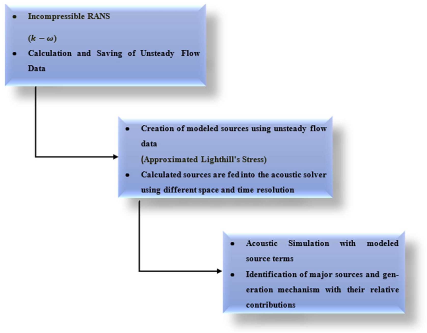
2.1.2. Acoustic Analogy

In 1950′s, Lighthill [42] extracted an accurate form of the heterogeneous wave equation based on Navier-Stokes and continuity equations. However, the extracted equation is limited since it estimates the sound waves only at unbounded domains and is incapable of considering reflection effects, absorption wave failure and extended wave dispersion over solid boundaries. Later, Curle [43] developed Lighthill’s model to include the presence of a solid object. Williams and Hawkings [44] improved the previous theories (Lighthill [42] and Curle [43]).

To analyze the noise generated by the flow, FW-H equation (Equation (8)) is used in addition to solving Navier-Stokes equations. This analogy includes all sound sources (monopole, dipole, and quadrupole) which is shown in Equation (8). This equation is basically a heterogeneous wave equation and is derived from the continuity equation and Navier-Stokes equations. Equation (9) is Lighthill stress tensor.

$$\begin{array}{l}\frac{1}{c_0^2}\frac{{\partial }^2{P}^{\prime }}{\partial t^2}-{\nabla }^2{P}^{\prime }=\underset{Quadrupole}{\frac{{\partial }^2}{\partial x_i\partial x_j}\left[T_{ij}H(f)\right]}-\underset{Dipole}{\frac{\partial }{\partial x_i}\left[\left[P_{ij}{n}_j+\rho u_i(u_n-v_n)\right]\delta (f)\right]}\\ +\underset{Monopole}{\frac{\partial }{\partial t}\left[\left[{\rho }_0{v}_n+\rho (u_n-v_n)\right]\delta (f)\right]}\end{array}$$

(8)

$$T_{ij}=\rho u_i{u}_j-{\tau }_{ij}+{\delta }_i{}_j\left[(p-p_{{}_0})-C_0{}^2(\rho -{\rho }_{{}_0})\right]$$

(9)

where $c_0$ denotes the speed of sound in a far field.$H\left(f\right)$ is Heaviside function and $\delta \left(f\right)$ denotes the Dirac Delta function.$u_n$ and $v_n$ are the fluid velocity in the direction normal to the integration surface and the surface velocity in the direction normal to the integration surface, respectively. Furthermore,${\tau }_{ij}$,${\delta }_{ij}$,$\rho$ and $P^{\prime }$ are respectively the viscous stress, Kronecker delta, the density and the sound pressure in the far field in $P^{\prime }=p-p_0$. In FW-H equation, $f=0$ indicates the source surface (cylinder and splitter plate), $f>0$ is unbounded space, $n_i$ represents the vertical unit vector towards outside the area, and $P_{ij}$ is the compressive stress tensor, which is defined as Equation (10) for a Stokes flow.

$$P_{ij}=p{\delta }_{ij}-\mu \left[\frac{\partial u_i}{\partial x_j}+\frac{\partial u_j}{\partial u_i}-\frac{2}{3}\frac{\partial u_k}{\partial x_k}{\delta }_{ij}\right]$$

(10)

The first term of the right of Equation (8) refers to quadrupole sources that is caused by unsteady shear stresses, and these are outside the source surface and have the least contribution in each period of sound generation, so it can be neglected. The quadrupole term is the distribution of the volume of sources defined by the Heaviside function $H\left(f\right)$. The second term, known as the dipole or loading source, is related to the forces applied to the surface of the body. The last term of the right of Equation (8) is for monopole sound source, also known as the thickness noise, caused by fluid displacement by the body surface in the flow field. In Equation (8), $\delta \left(f\right)$ represents the mono-and dipole sources. To solve the FW-H equation, the free-space Green’s function is utilized to compute the sound pressure at the receiver location x. Acoustic pressure is defined by Equation (11), where the $Q$, $L$, and $T$ components represent the quadrupole, loading (dipole), and thickness (monopole), respectively. These parameters are described in Equations (12)–(14), respectively [44,45]. Since quadrupole sources have not an effective role in noise generation, they are ignored.

$$P^{\prime }(\overrightarrow{x},t)=P_Q^{\prime }(\overrightarrow{x},t)+P_T^{\prime }(\overrightarrow{x},t)+P_L^{\prime }(\overrightarrow{x},t)$$

(11)

$$P_Q^{\prime }(\overrightarrow{x},t)=\frac{1}{4\pi }\left(\left(\frac{{\partial }^2}{\partial x_i\partial x_j}\right){{\displaystyle \underset{V}{\int }\left[\frac{T_{ij}}{\left(r\left(1-M_r\right)\right)}\right]}}_{ret}dV\right)$$

(12)

$$P_T^{\prime }(\overrightarrow{x},t)=\frac{1}{4\pi }\left(\left(\frac{\partial }{\partial t}\right){{\displaystyle {\int }_S\left[\frac{{\rho }_0{n}_i\left(\left(1-\frac{\rho }{{\rho }_0}\right)v_i+\frac{\rho u_i}{{\rho }_0}\right)}{\left(r\left(1-M\right)\right)}\right]}}_{ret}dS\right)$$

(13)

$$P_L^{\prime }(\overrightarrow{x},t)=\frac{1}{4\pi }\left(\left(-\frac{\partial }{\partial x_i}\right){{\displaystyle \underset{S}{\int }\left[\frac{P_{ij}{n}_i+\rho u_i\left(u_{i_n}-u_{j_n}\right)}{\left(r\left(1-M\right)\right)}\right]}}_{ret}dS\right)$$

(14)

Here the subscript ($r_{et}$) means for the retarded time, and M is local Mach number.

The radiated sound, based on unsteady force on the body in the calculations, is written as [46]:

$$P\prime (x,t)=-\frac{1}{4\pi }\frac{\partial }{\partial x_i}\left[\frac{F_i}{r}\right]=\frac{1}{4\pi c_0}\frac{x_i}{r^2}\left[\frac{\partial F_i}{\partial t}\right]$$

(15)

where $r$ is the observer distance from the sound source and $\frac{\partial F_i}{\partial t}$ is the time gradient of unsteady force on the body.

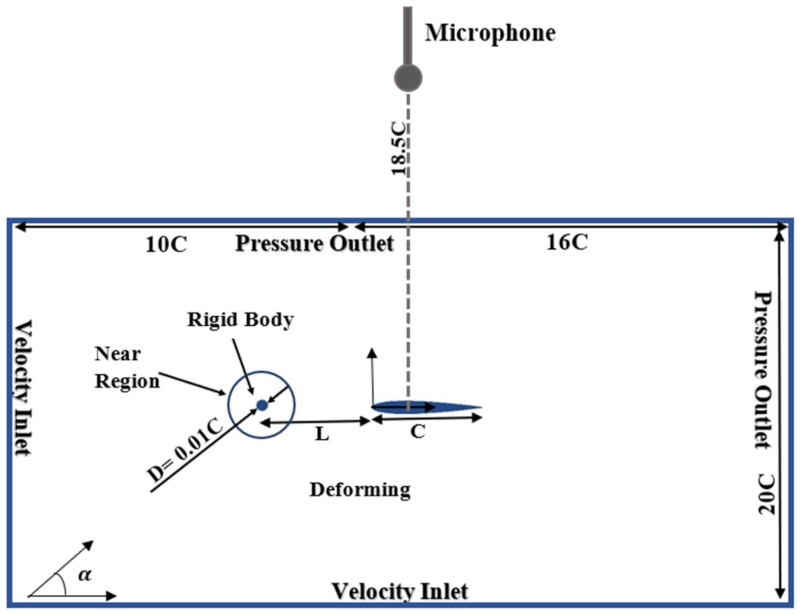
2.2. Geometric Model

In the present study, the geometric model is adopted from the experimental model proposed by Jacob et al. [19]. Thus, an airfoil is of NACA 0012 type with a 0.1 m (C = 0.1 m) chord is located at the downstream side of a rod at a distance equal to the airfoil cord (L = 1 C) with a diameter of 0.1 times the airfoil chord (D = 0.1 C). The Reynolds number is 48,000 based on the rod diameter, and 480,000 based on the airfoil chord, and the Mach number is 0.2. Furthermore, between the rod and the airfoil in the vertical direction ($y$), there is a $y$ = 2 mm shift between the rod axis and the airfoil chord. The x-axis is parallel to the flow, and the y-axis is perpendicular to the flow in downward and upward directions. The origin of coordinates is also located at the leading edge of the airfoil. A literature review shows that the rectangular domain with the intended dimensions is suitable for solving this problem (Figure 1) [30,31]. To measure the aerodynamic noise of the flow, a microphone is embedded at the top and center of the airfoil at a distance of 18.5 C. Figure 1 illustrates a schematic of computational domain along with the boundary conditions.

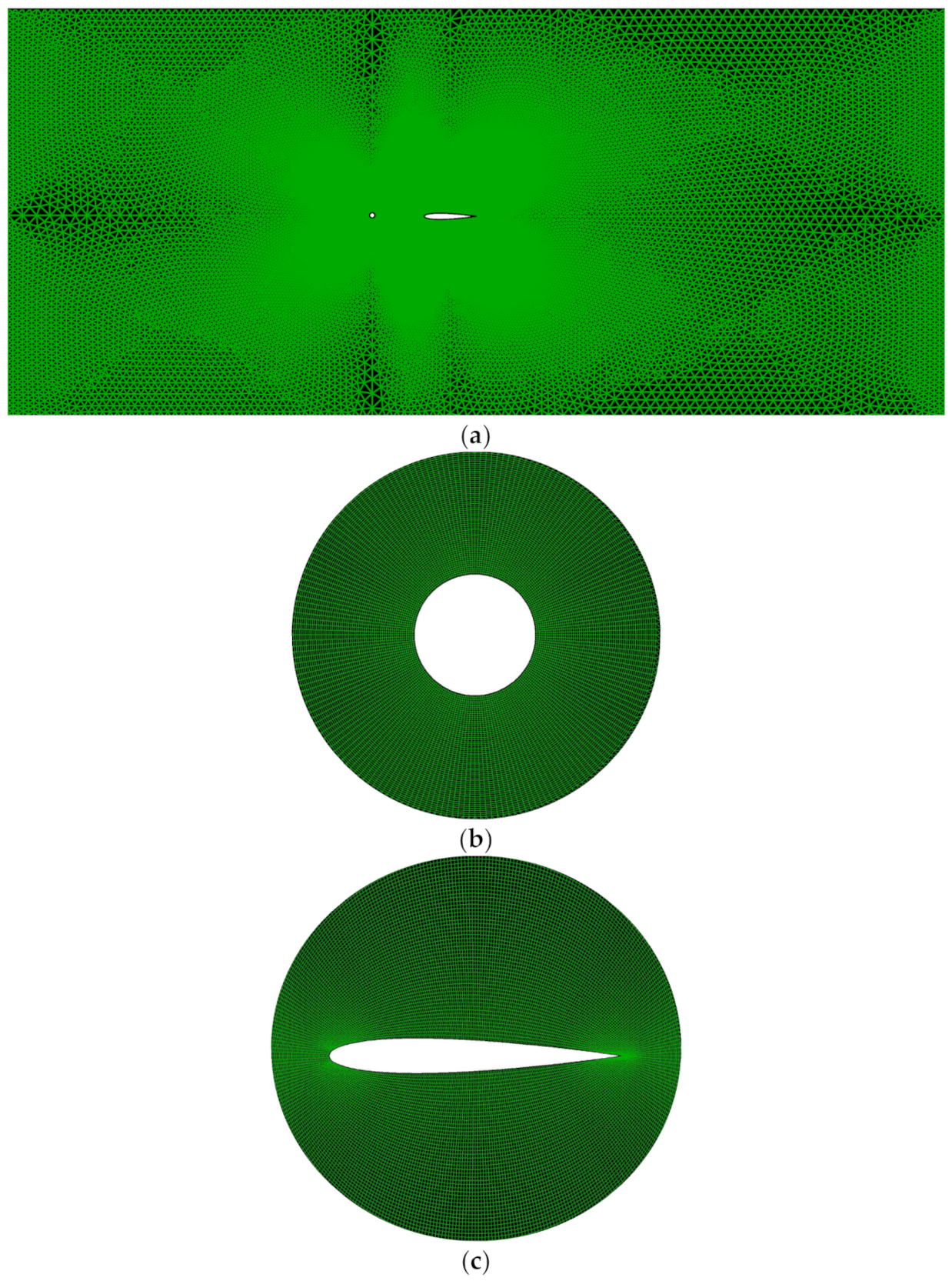
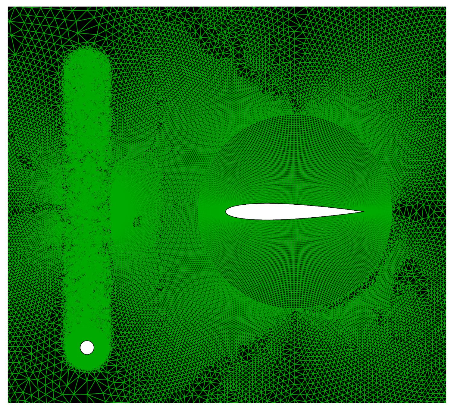
2.3. Meshing Process

Considering the fact that this paper aims at investigation of the noise generated through the transient fluid flow, a precise estimation of flow turbulence is of high importance. To accurately estimate extreme velocity gradients, a precise meshing is deemed necessary and vital especially near the wall. Given that the rod has vibrational movements in the vertical direction to the flow, meshing of the calculation field is depicted as triangles in Figure 2a. The unstructured mesh has a lower computational cost than structured mesh. However, they have almost the same accuracy. Moreover, since the recorded noise is generated from variations of pressure on a solid surface, the meshing around the rod and the airfoil must be finer, and to avoid sudden variations in mesh density, the meshing of the field around the rod and the airfoil is quadrilaterals as in Figure Figure 2b,c. The circumference of rod and airfoil is discretized by 200 and 300 nodes, respectively. To assess the quality of generated mesh, a validation study is presented in

Table 2. Properties of the Computational Grid.

Case	${\mathit{y}}_{\mathit{m}\mathit{e}\mathit{a}\mathit{n}}^{+}$
-	Rod	Airfoil
Coarse mesh	29.787	38.475
Medium-sized mesh	12.474	14.35
Fine mesh	3.212	3.894
Rousoulis et al. [29]	$y^{+}<3$

. In the three examined density levels, $y^{+}$ is investigated to determine the best mesh for simulation because it plays an important role in estimating the flow behavior in the boundary layer. $y^{+}$denotes the non-dimensionalized distance of the grid points from the wall and defined as $y^{+}=\raisebox{1ex}{$u_{\tau }y$}\!\left/ \!\raisebox{-1ex}{$v$}\right.$ ($u_{\tau }$: friction velocity and y: distance from the wall).

2.4. Solver Settings

ANSYS-Fluent commercial software has been used for the numerical analysis of the flow. URANS have been used for solving the governing equations. Two-equation turbulence models are the simplest forms of turbulence models. Two-equation turbulence models allow the determination of both the turbulent velocity and length scales by solving two separate transfer equations [47]. The k-ω-SST turbulence model has been used to accurately estimate viscosity eddies. Stability, economy, and appropriate precision for a wide range of turbulent flows explain its popularity in the simulation of turbulent heat transfer and flow in the industry [10,31,40,45,48,49,50,51]. To provide for a comparison of the present numerical solution results with the empirical research conducted by Jacob et al. [19], all the applied dimensions, parameters, and boundary conditions have been considered exactly according to the conditions of the empirical research. A constant flow at the speed of 72 m/s has been assumed at the inlet boundary. For solution, simple pressure-velocity coupling with Least Squares Cell-Based Gradient discretization was used. Furthermore, second-order spatial discretization approach was used for pressure and momentum. Moreover, first-order spatial was employed for turbulent kinetic energy and dissipation rate. For the unsteady simulation process, a time step of 0.0001 s is used and the total simulation time is 0.8 s with 50 inner iterations at each time interval. After reaching the aerodynamic force and convergence diagram to an iterative pattern and ensuring its stability (0.35 s) (Figure 3), the FW-H analogy is coupled with a flow solution, and the data are extracted at the end of the analysis (0.8 s). The convergence condition in every governing equation is for residuals to reach 10⁻⁵. Moving mesh is implemented for the rigid body (rod) and near region, whereas the outer of near region is kept stationary (deforming region) (Figure 1). As previously mentioned, FW-H solution has been used in this study in order to extract the noise pressure level and the aerodynamic noise. Moreover, a frequency resolution, equal to the sampling frequency (i.e., 10 kHz), is employed for the FW-H results. Since the literature review has shown that 2D models are also reliable, this model is used in this study to extract noise and to simulate flow structure [26,31,33,45,52]. The numerical procedure outlined above for predicting the generation and propagation of aeolian tone noise is summarized in Figure 4 [53].

3. Results and Discussion

First, the results’ becoming independent of the grid is addressed. Then validation of acoustics and aerodynamic parameters is made to examine the validity of the current study. Eventually, acoustic control and flow disturbances are addressed by using the rod vibration.

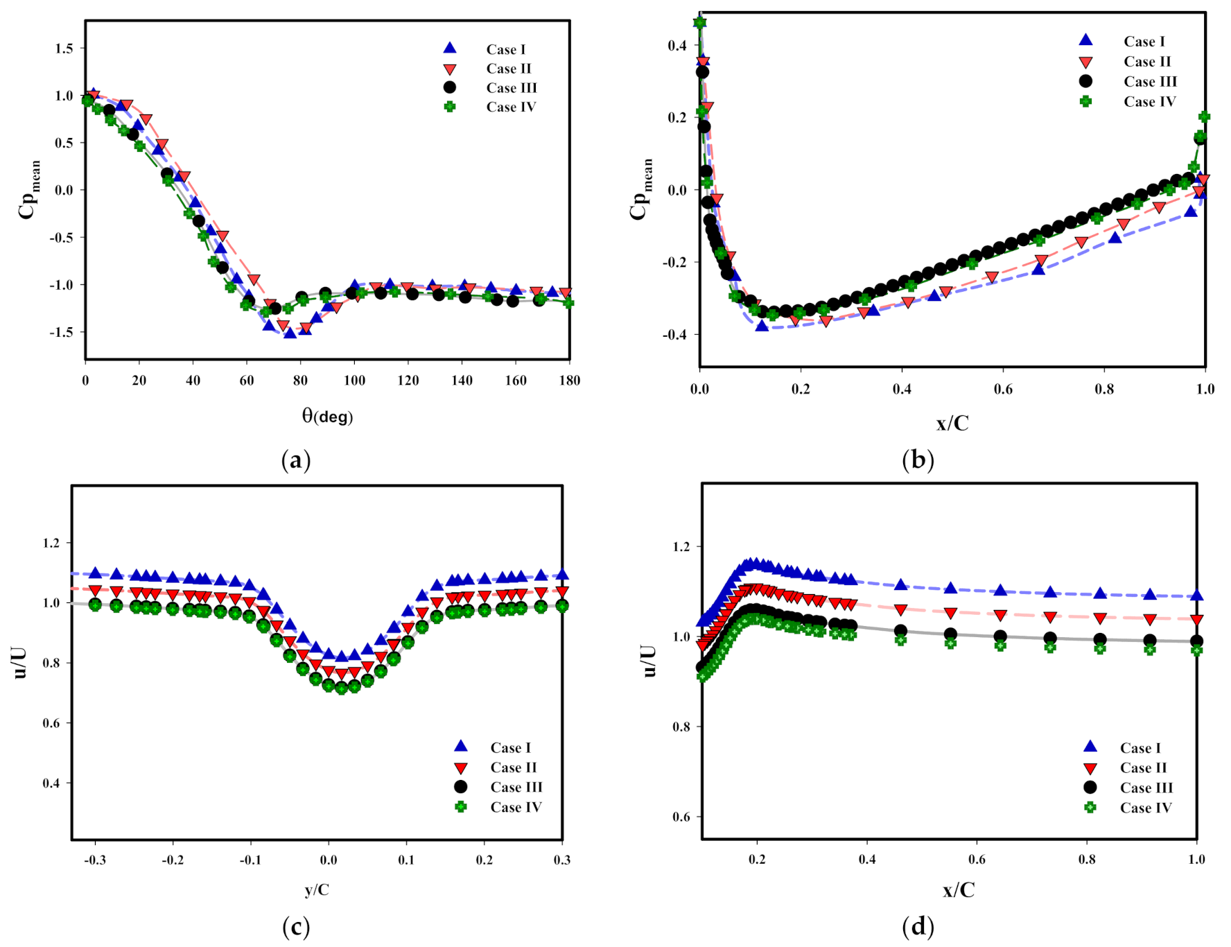
3.1. Examination of Independence from the Grid

To make sure of the conducted meshing and the number of calculation cells considered, dependence from the grid is made for the results of the numerical analysis. To this aim, the meshing of the measurement zone has been performed in multiple cases around the Rod-Airfoil, the sound pressure level (SPL), and the peak amplitude Strouhal number, and the mean pressure parameter around the rod and airfoil and mean velocity parameter are obtained as the most important results. Meshing has been carried out with different numbers of computational cells. In

Table 3. Examining independency of the problem results from the grid.

Case	Elements	Number of Cells	Body	SPL	St
I (Coarse mesh)	Quadrangular	4800	Rod	32
			Airfoil	40	0.361
	Triangular	36,000
			Rod-Airfoil	40
II (Medium-sized mesh)	Quadrangular	9300	Rod	64
			Airfoil	70	0.274
	Triangular	69,000
			Rod-Airfoil	72
III (Fine mesh)	Quadrangular	14,000	Rod	88
			Airfoil	99	0.2120
	Triangular	95,000
			Rod-Airfoil	99
IV	Quadrangular	20,000	Rod	89
			Airfoil	100	0.2118
	Triangular	125,000
			Rod-Airfoil	100

, the maximum value of SPL (i.e., the peak value of the noise spectrum (NSP) recorded by embedded microphone) is calculated according to the contribution of noise generated by the rod and airfoil in the total of NSP for different numbers of calculation cells. Strouhal number that occurs in the NSP is also recorded. Equation (16) presents the calculation of SPL and Equation (17) demonstrates the calculation of the Strouhal number. In Equation (16), $P_{rms}^{\prime }$ denotes the root mean square of pressure disturbances, and $P_{ref}$ is equal to 2 × 10⁻⁵ (pa). It is evident that following the variations in the meshing of the solution field from case I to case III, the NSP and the peak amplitude Strouhal number show significant changes; however, by increasing the number of cells from case III to case IV, the results do not undergo much change. Maximum SPL recorded from the Rod-Airfoil configuration is equal to the dominant sound source. It is clear that airfoil is the predominant source.

$$SPL(db)=20\log (\frac{P_{rms}^{\prime }}{P_{ref}})$$

(16)

$$St=\frac{fD}{U}$$

(17)

Figure 5 depicts the results of mesh study for the average pressure coefficient around the rod and the airfoil and velocity at x/C = − 0.25 and x/C = + 0.25. Clearly, in case (I) and (II), the pressure coefficient and velocity are of relatively greater value; however, with a finer meshing in case (III), this value is decreased. By increasing the number of trihedral and tetrahedron grids in case (IV), no significant change occurs in the results in comparison with case (III). According to the results of Table 2 and Figure 5, it is clear that the third and fourth cases are slightly different in predicting the results, which can be ignored. On the other hand, fining the mesh lead to increasing the computational cost. Therefore, considering the acoustic and the aerodynamic results and reduce the computational cost, the grid in case (III) is appropriate for the present investigation.

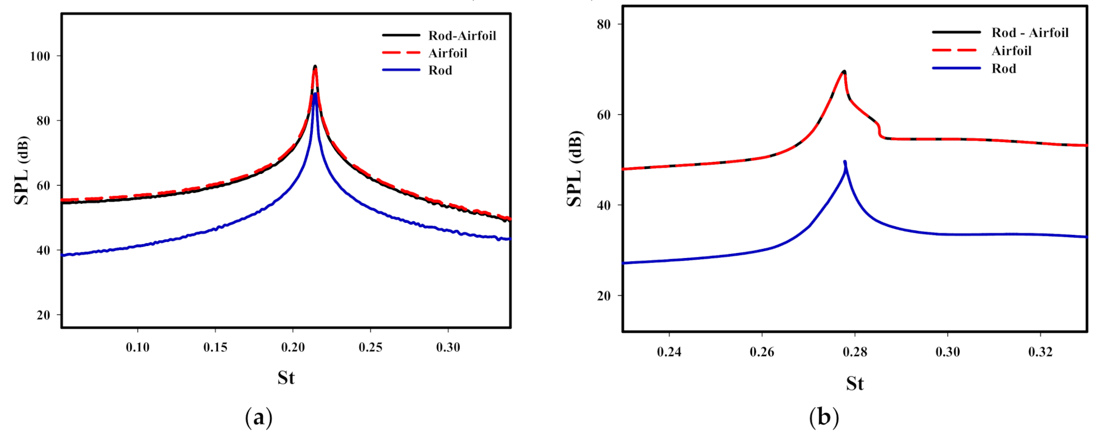
3.2. Validation of Results

Penetration of vortex structures at the airfoil leading edge results in the generation of powerful acoustic sources such as the noise generation mechanism in turbomachinery in a study by Homicz and George [15]. Hence, the leading edge significantly has the most contribution to the generation of noise in comparison with the rod and the trailing edge. Validation of the acoustic results are achieved using the SPL and the Strouhal number (Figure 6) in comparison with experimental results of Jacob et al. [19]. The peak amplitude Strouhal number, equal to 0.2120, is stated as Equation (17) at a frequency of 1526 Hz. The obtained value has a trivial difference with that of the empirical study, which is equal to 0.192. Furthermore, the obtained NSP in the numerical method is 99 dB, the value which is 6.5 dB higher than that in the results of Jacob et al. [19]. The discrepancy is due to the nature of the present modeling. 2D models do not take into account the features of experimental and 3D models, so they make mistakes in correctly estimating the separation position, which leads to more estimates of the amount of lift force and its fluctuations [54,55]. On the other hand, due to the significant contribution of lift in noise production, this leads to a higher estimate of SPLs than experimental and 3D studies. Another feature of 2D models is that it does not take into account the spanwise effect, which leads to a higher estimate of the frequency (St) at NSP, according to what is obtained in Figure 6. The difference in SPL between the present model and the experimental model, in other Strouhal numbers, is due to the URANS method, which does not consider smaller eddies in the near wake region [33,52,56,57]. Although the flow of Rod-Airfoil in high Reynolds numbers is inherently 3D, 2D approaches can still illustrate the key aspects of vortex shedding with significant cost reductions. Furthermore, despite the differences and shortcomings of this model, its prediction capability is high, and the simulated SPL is reasonably consistent with the experimental results.

Evaluation of the average velocity is an important parameter for examining the flow pattern. Consequently, this study attempts to validate this parameter as one of the most important aerodynamic parameters. The average velocity validation has been achieved at two points in the flow: $\frac{X}{C}=-0.25$ and $\frac{X}{C}=+0.25$.$\frac{X}{C}=+0.25$ and $\frac{X}{C}=-0.25$ have been devised as perpendicular to the airfoil and at the rod wake respectively. In Figure 7a, the minimum value of $\frac{u_{mean}}{U_0}·\frac{X}{C}=-0.25$ in the experiential study equals 0.701, and its minimum value in the numerical study is 0.721; the relative error is 1.6%. As shown in Figure 7b, the average velocity difference at $\frac{X}{C}=+0.25$ between the empirical and the numerical methods is 5.9%. It is evident that the present numerical method has a trivial difference with LES, and both patterns are the same as that of the empirical study with very little difference. After reviewing the results and the acceptable validation provided, Computational Fluid Dynamics (CFD) prediction is possible for further sufficiently accurate investigation of the flow pattern for the present study.

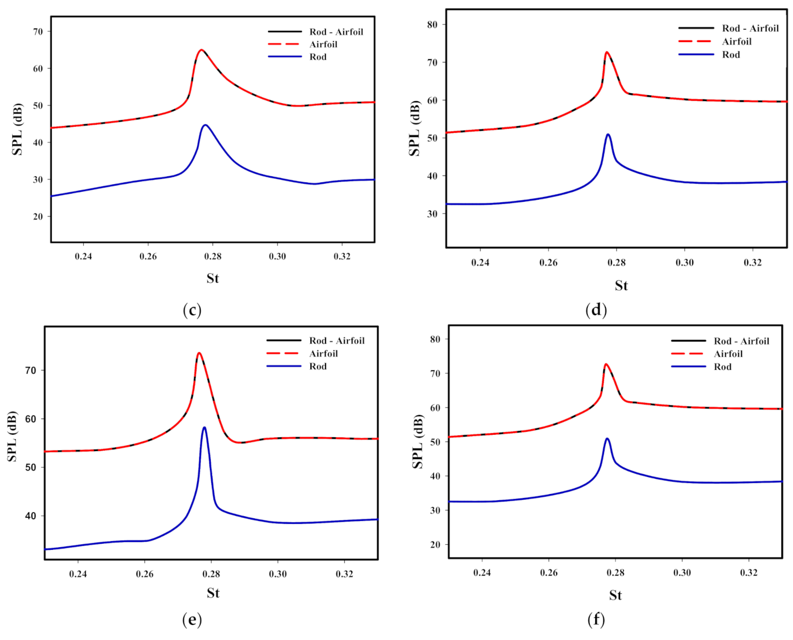
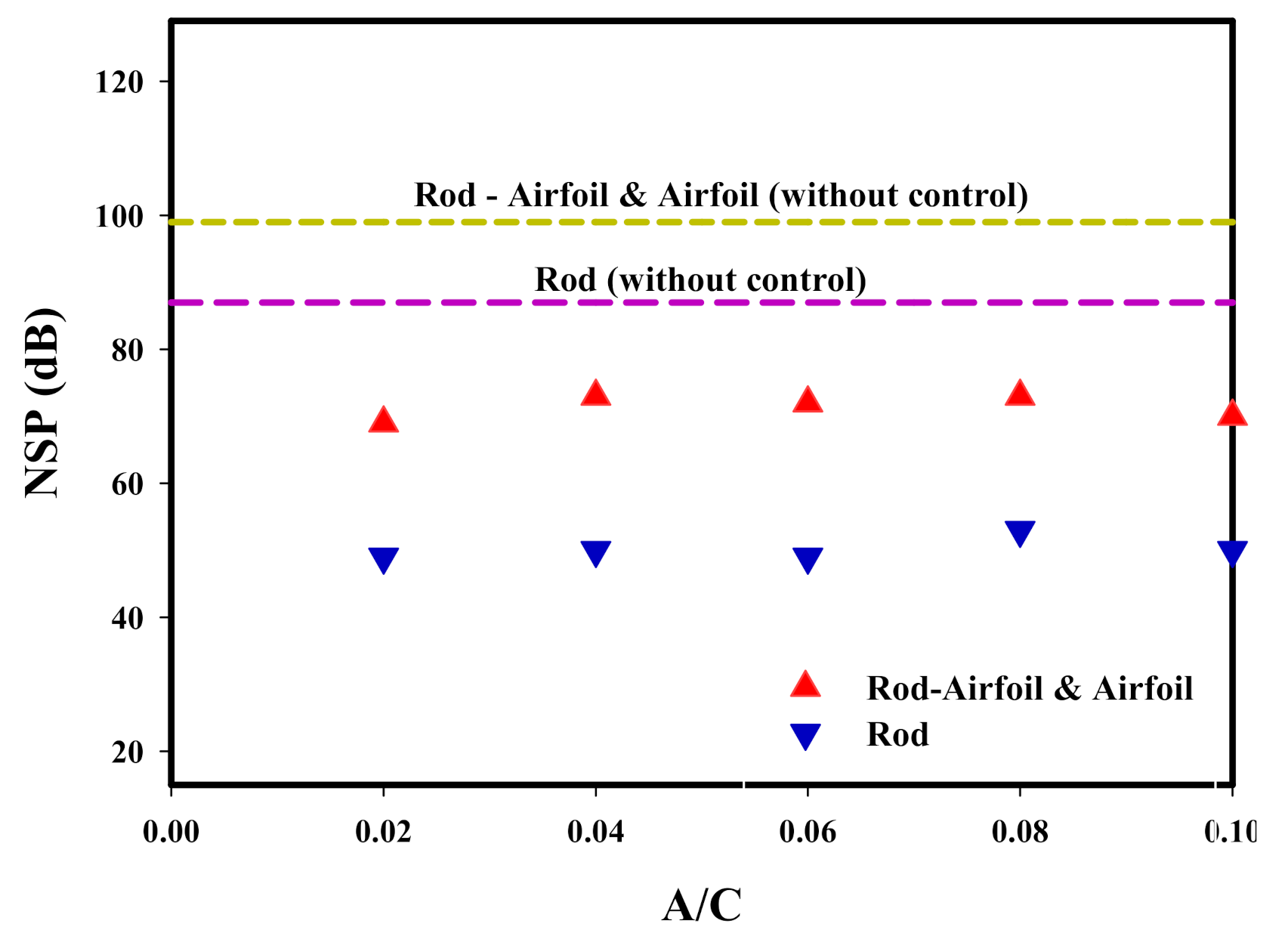
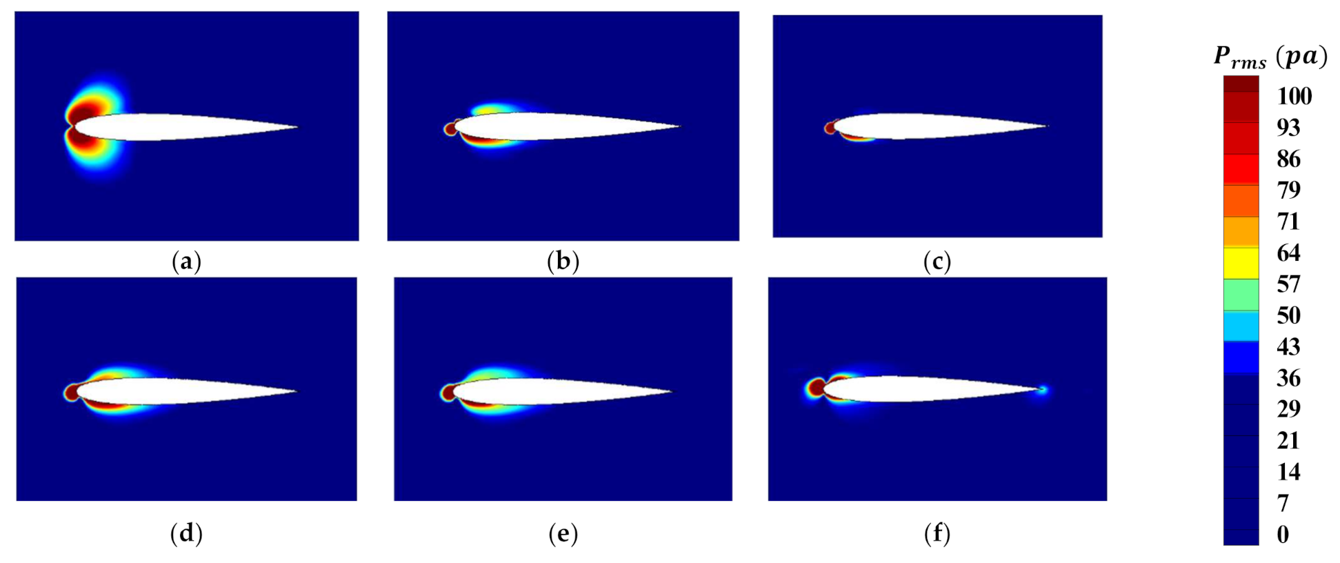
3.3. Applying Control and Study of Its Effect on Aerodynamic Noise

According to Homicz and George study [15], it was found that the leading edge is the most important source of noise generation. Therefore, in the present study, the effect of the open-loop vibrating rod control method is investigated. In other words, the rod will have an open-loop sinusoidal motion perpendicular to the flow whose range varies from 0.02C to 1C. The frequency of harmonic motion is 5 Hz.

The mesh motion is shown in Figure 8 by moving the rod, while A = 1C is considered as the displacement.

In the following, the role of the introduced control method on aeroacoustic characteristics is examined. Figure 9 illustrates the SPL variations by applying vibration to the rod and increasing the amount of rod displacement. As is observed, applying vibration has resulted in a drop in the aerodynamic noise. Since the dominant noise in the Rod-Airfoil combination is due to flow disturbance at the downstream side of the rod on the airfoil leading edge, the rod motion perpendicular to the flow causes the flow at the downstream side of the rod to also distance away from the airfoil leading edge and lead to flow disturbance reduction around the edge. Eventually, the pressure fluctuations at the airfoil attack surface also decrease. Hence, it is expected that noise also decreases with rod motion perpendicular to the flow. The extracted charts demonstrate the dominance of the airfoil noise. Clearly, the recorded airfoil noise equals that of Rod-Airfoil and the rod noise without applying control is 10 dB less than the Rod-Airfoil noise. Applying oscillation to the cylinder in the range of $A\le 0.1C$ generally reduces the SPL, caused by the Rod-Airfoil, airfoil and rod; by about 22 dB (Figure 10). By applying oscillation to the rod, the vortex shedding phenomena are changing which leads to an increase in the peak amplitude Strouhal number (about 20%).

To evaluate the role of aerodynamic forces on a bluff body in noise generation, magnitude of root mean square (rms) sound pressure ($\tilde{P}=\raisebox{1ex}{$P_{rms}^{\prime }$}\!\left/ \!\raisebox{-1ex}{$\rho U_{\infty }^2$}\right.$) are presented due to the lift and drag fluctuations for the 0 C–0.1 C variations range in Figure 11 and Figure 12. These plots show the share of the acoustic pressure of the lift and drag from the total radiated pressure from configuration based on Equation (15), drawn separately to better understand the values. According to Figure 11, it is evident that the sound waves radiates by the lift fluctuations at the direction $\pm {90}^{°}$ from the sound source. It is also shown in Figure 12 that the direction of the sound field waves radiates by the drag fluctuations are $0^{°}$ and ${180}^{°}$. From Figure 11 and Figure 12, it can be seen that the noise emitted by the body is dipolar, which is consistent with Curl’s [36] result. The peaks of the graphs follow their respective forces. The major changes in $\tilde{P}$ are related to changes in aerodynamic forces. It is clear that in all cases, the magnitude of $\tilde{P}$ for the sound source from the drag signal is small than from the lift signal. This is due to the small amplitude of drag fluctuation, as compared to the amplitude of lift fluctuation. It can be found that in the interval ${30}^{°}–{150}^{°}$ and ${210}^{°}–{330}^{°}$, the highest proportion of noise produced is due to lift fluctuations and at angles outside this range, the highest contribution is related to drag fluctuations. This result may indicate that if the microphone approaches $0^{°}$ and ${180}^{°}$ angles, the drag contribution to noise production will increase. Since the noise received from the drag fluctuations is far below the lift, it is expected that a lower SPL will be recorded. Sun et al. [58] have shown that with the microphone approaching angles approaches $0^{°}$ and ${180}^{°}$ the SPL is significantly reduced. Moreover, with respect to Figure 11, where the noise of the rod is less than that of the Rod-Airfoil, the two graphs also show that the rod has less sound pressure fluctuations.

The changes in NSP are examined by applying vibration to the cylinder for intervals greater than 0.1C ($0.1C<A\le 1C$). Figure 13 shows that increasing displacement decreases the NSP. Increasing the displacement reduces the role of the leading edge in noise generation, and along with that, the trailing edge also becomes a factor for noise generation. In A = 1C, the NSP is reduced by nearly 35 dB. The noise level changes in the range of $0.1C<A\le 1C$ are not significant, so it is expected that the change pattern of noise will be repeated by increasing the displacement rate in $1C\le A$. The reason for this behavior is that the rod is far enough away from the chord at $A=0.2C$, and the transient flow of the rod has low effect on the airfoil, so it is expected that increasing the amplitude more than $2C$ has no significant effect on the noise level.

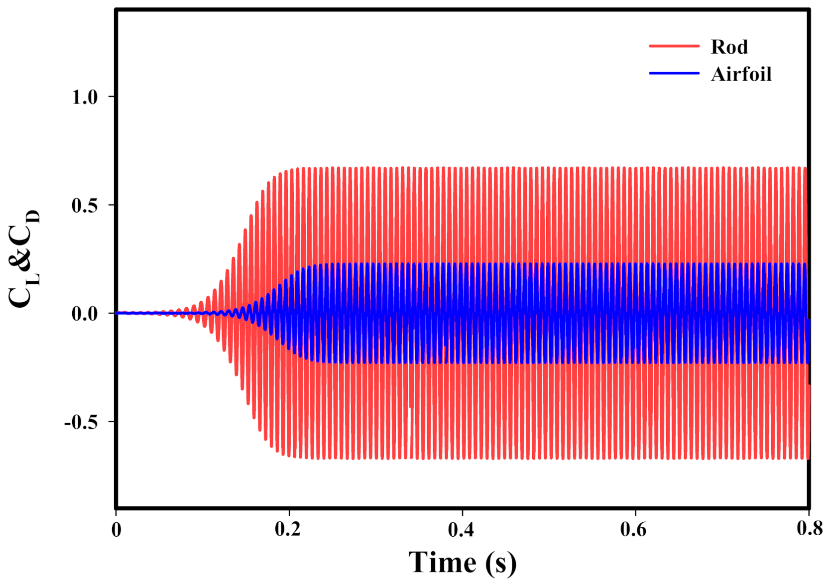
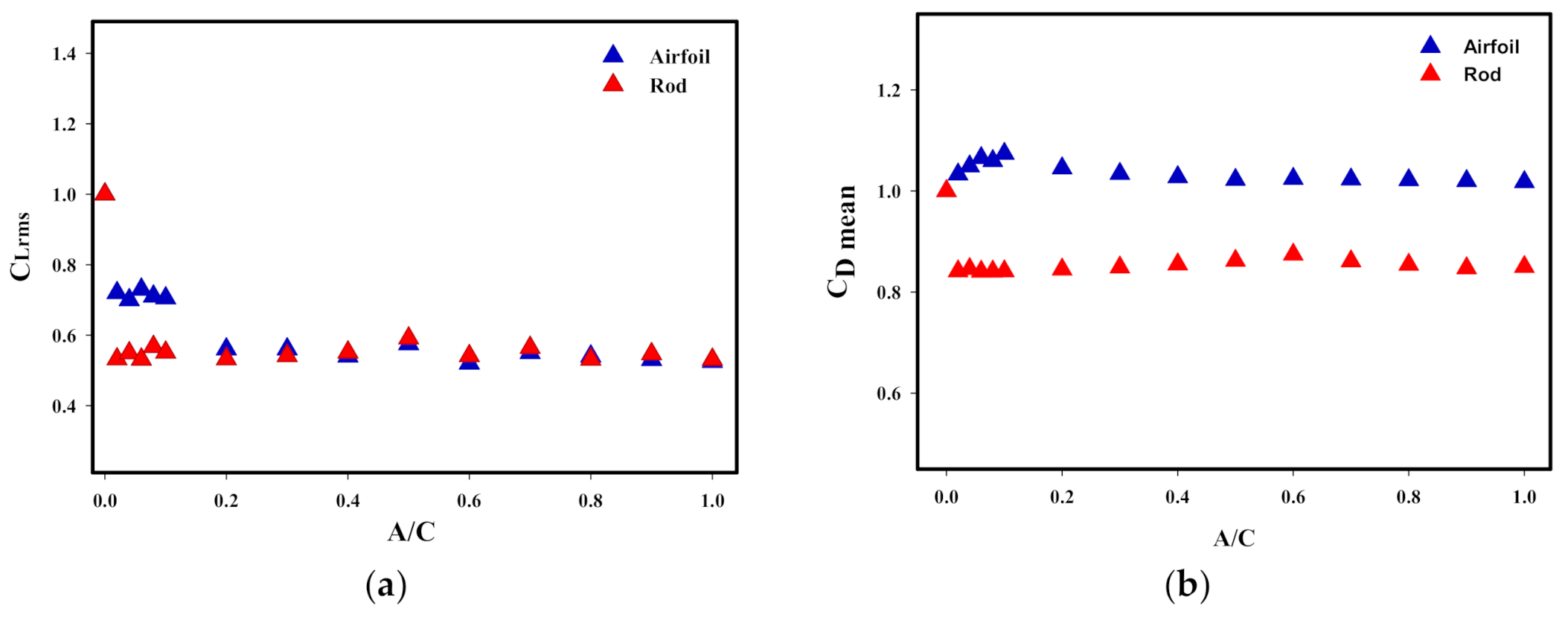
3.4. Effect of Flow Control on Aerodynamic Coefficients

Hereafter, the control method’s effect on dimensionless coefficients of lift and drag will be discussed. Hence, lift and drag coefficient values of the Rod-Airfoil have been produced. The average values are not indicative of the generated sound, But the generated sound field is due to fluctuations of the forces applied to the bluff body. According to the results of Figure 11 and Figure 12, the current position of the microphone, drag has the lowest domain of noise generation. Given the fact that dipole noise is a function of $C_{L_{rms}}$ then variations in $C_{L_{rms}}$ are examined by applying control. Mean drag, known as a structural destructive force, and mean lift have also been investigated. rms and mean values have been reviewed as absolute values according to Equations (18)–(21). The values have been recorded in the figures studied as compared to the case with no control.

$${\mathrm{C}}_{{\mathrm{L}}_{\mathrm{rms}}}=\frac{\left|{\mathrm{C}}_{{\mathrm{L}}_{\mathrm{rms}\mathrm{X}}}\right|}{\left|{\mathrm{C}}_{{\mathrm{L}}_{\mathrm{rms}\mathrm{X}=0}}\right|}$$

(18)

$${\mathrm{C}}_{{\mathrm{D}}_{\mathrm{mean}}}=\frac{\left|{\mathrm{C}}_{{\mathrm{D}}_{\mathrm{mean}\mathrm{X}}}\right|}{\left|{\mathrm{C}}_{{\mathrm{D}}_{\mathrm{mean}\mathrm{X}=0}}\right|}$$

(19)

$${\mathrm{C}}_{\mathrm{L}}{}_{\mathrm{m}\mathrm{e}\mathrm{a}\mathrm{n}}=\frac{\left|{\mathrm{C}}_{{\mathrm{L}}_{\mathrm{mean}\mathrm{X}}}\right|}{\left|{\mathrm{C}}_{{\mathrm{L}}_{\mathrm{mean}\mathrm{X}=0}}\right|}$$

(20)

where ${\mathrm{C}}_{{\mathrm{L}}_{\mathrm{rms}\mathrm{X}=0}}$, ${\mathrm{C}}_{{\mathrm{D}}_{\mathrm{mean}\mathrm{X}=0}}$, and ${\mathrm{C}}_{{\mathrm{L}}_{\mathrm{mean}\mathrm{X}=0}}$ represent the fluctuations of the lift, the mean drag, and lift in the uncontrolled case, respectively. Moreover, ${\mathrm{C}}_{{\mathrm{L}}_{\mathrm{rms}\mathrm{X}}}$, ${\mathrm{C}}_{{\mathrm{D}}_{\mathrm{mean}\mathrm{X}}}$ and ${\mathrm{C}}_{{\mathrm{L}}_{\mathrm{mean}\mathrm{X}}}$ respectively indicate the lift fluctuations, mean drag, and lift for the studied cases ($0.02C<A\le 1C$).

Figure 14a has illustrated the airfoil and the rod lift coefficient fluctuation values. It is observed that $C_L{}_{rms}$ has generally decreased. Since variations in lift coefficient fluctuations are dominant, then it is expected that they will be similar to variations in the sound pressure level. It may be observed in this figure that the minimum recorded value of the lift coefficient fluctuations occurs in the airfoil at $0.2C\le A\le 1C$, which has decreased by about 48% compared to the case with no control. The amount of reduction in the rod’s lift coefficient fluctuations at $\frac{A}{C}=1$ has decreased by about 46% in comparison to the case with no control. Figure 14b illustrates the averaged drag coefficient. The results generally indicate increase in the airfoil’s average drag coefficient after applying control by 7% at $0.02C\le A\le 0.1C$ and 2% at $0.2C\le A\le 1C$, and reduction in the rod’s average drag coefficient by 16%. Moreover, vibration in the rod increases the mean lift coefficient, which is aerodynamically desirable (Figure 14c).

Then, further investigation of flow pattern and the force applied to the system will be made. Since the flow characteristics in 0.2C ≤ A ≤ 1C are similar to 0.02C ≤ A ≤ 0.1C, so the flow characteristics are only examined for the second range. Figure 15 has presented the average static pressure. It is highly important to study static pressure contours because it clearly demonstrates the greatest static pressure variation domains is surrounded the airfoil. Pressure variations around the airfoil lead to variations in drag and lift forces. It is clear from the figure that the harmonic motion of the rod causes the pressure distribution pattern to change, which increases the pressure difference in both sides of the airfoil.

Unsteady pressures which support lift dipole are the most important and the most common factor in the generation of noise [43]. This unsteadiness is mainly created in the vicinity of the solid boundary and its surrounding. Figure 16 has depicted pressure disturbance contour (P_rms). These values are obtained from $P_{rms}=\sqrt{\frac{1}{N}{\displaystyle \sum }_{n=1}^N{\left(P-\overline{P}\right)}^2}$. As is evident in the figure, the highest RMS pressure level occurs at the airfoil leading edge. Nevertheless, this pressure stress significantly helps the noise, for this stress is located adjacent to the solid boundary. Hence, it can support dipole sources, and it is in fact not relevant to the quadrupole shape. The maximum recorded intensity can indicate the source of the noise. it is necessary to mention the emitted noise does not depend only on the amplitude of the pressure fluctuations, i.e., the coherence of the fluctuations and the shape of the close by solid surface may play a role, but pressure fluctuations are predominant It is evident from Figure 16 that the airfoil leading edge is the cause of sound generation and this zone of tension is located adjacent the airfoil due to the motion of the rod. It should be noted that after the application of control, the area of $P_{rms}$ decreases by increasing the amount of rod displacement so that it would decrease by nearly 50% at A/C = 0.1. Considering the previously discussed issues, if the airfoil is not located at the downstream side of a bluff body, its trailing edge noise might be dominant. It is known that at x/C = 0.1, the intensity of $P_{rms}$ is also generated at the edge of the airfoil trailing edge. This indicates that the noise recorded in Figure 10 for A/C = 0.1, in addition to the leading edge, is also due to the trailing edge.

Vorticity contours can perfectly illustrate the boundary layers, the shear layer growth, and the instability of vortices that eventually turn into von Kármán street. The occurrence of this periodic structure is the main cause of the pressure difference, the fluctuations of the forces applied to the system, and the noise generation. Figure 17 show the vorticity contours after applying the control method ($0C\le A\le 0.1C$). Vorticity contours are extracted 0.45 s after the start of the analysis. According to Figure 17, in the case of A = 0C, it is clear that the turbulent flow has been applied to the leading edge, which has caused the leading edge to be dominant in noise generation. Vibration in the rod causes the vortex shedding phenomena to change due to vortex roll-up distance. According to Figure 17 which shows vibration apply in the rod, the created vortexes occur smaller and closer to the back surface of the rod, resulting in a dramatic increase in the St [59] due to what happened in Figure 9. It is clear that the vibration in the rod has caused the downstream vortex of the rod not to penetrate on the leading edge as in an uncontrolled case. So, the fluctuations of the flow near the leading edge are reduced. The flow characteristics are relatively similar in different cases, so the noise reduction is relatively same for different cases. An important point in A = 0.1C is increasing the vortex size created at the trilling edge which increases its role in noise generation. This result can be seen in Figure 16, with increasing pressure fluctuations in the mentioned region. Accordingly, similar results are expected to occur at A = 0.1C, in other words, increasing the role of the trailing edge in increasing noise along with reducing the role of the leading edge.

4. Conclusions

This study demonstrates that the vibrating rod method is capable of reducing the generated noise. This method is potentially used to reduce the noise in vertical-axis wind turbines when they are located downstream of a bluff body. As a general and final conclusion, it may be stated that any factor contributing to control of the airfoil leading edge vortices will result in noise reduction. For example, corrugating the airfoil leading edge and rotating the rod (according to the literature), controlled or deviated vortices. Noise reduction capability is advantageous when these practical programs are truly taken into consideration. Currently, the experimental data on the effect of the vibrating rod on the Rod-Airfoil aeroacoustics are not available; therefore, reliable evaluation of the proposed approach is optimistic for real cases. Moreover, 3D simulation for considering the effects of spanwise with the LES turbulence model can be a useful idea to ensure the results.

In this study, the performance of 2D models was evaluated and the results were sufficiently reliable. However, to better understand and improve these models, our team plans to evaluate Gaussian function and 3D models for more complex configurations in future studies.

References

1. Soltani, M.; Kashkooli, F.M.; Dehghani-Sanij, A.; Kazemi, A.; Bordbar, N.; Farshchi, M.; Elmi, M.; Gharali, K.; Dusseault, M.B. A comprehensive study of geothermal heating and cooling systems. Sustain. Cities Soc. 2019, 44, 793–818. [Google Scholar] [CrossRef]
2. Dehghani-Sanij, A.; Soltani, M.; Raahemifar, K. A new design of wind tower for passive ventilation in buildings to reduce energy consumption in windy regions. Renew. Sustain. Energy Rev. 2015, 42, 182–195. [Google Scholar] [CrossRef] [Green Version]
3. Gharali, K.; Gharaei, E.; Soltani, M.; Raahemifar, K. Reduced frequency effects on combined oscillations, angle of attack and free stream oscillations, for a wind turbine blade element. Renew. Energy 2018, 115, 252–259. [Google Scholar] [CrossRef]
4. Fredianelli, L.; Licitra, G.; Gallo, P.; Palazzuoli, D. The suitable parameters to assess noise impact of a wind farm in a complex terrain: A case-study in Tuscan hills. In Proceedings of the Euronoise Prague, Prague, Czech Republic, 10–14 June 2012. [Google Scholar]
5. Barlas, E.; Zhu, W.J.; Shen, W.Z.; Dag, K.O.; Moriarty, P. Consistent modelling of wind turbine noise propagation from source to receiver. J. Acoust. Soc. Am. 2017, 142, 3297–3310. [Google Scholar] [CrossRef] [PubMed] [Green Version]
6. Oerlemans, S.; Sijtsma, P.; López, B.M. Location and quantification of noise sources on a wind turbine. J. Sound Vib. 2007, 299, 869–883. [Google Scholar] [CrossRef]
7. Botha, J.; Shahroki, A.; Rice, H. An implementation of an aeroacoustic prediction model for broadband noise from a vertical axis wind turbine using a CFD informed methodology. J. Sound Vib. 2017, 410, 389–415. [Google Scholar] [CrossRef] [Green Version]
8. Maizi, M.; Mohamed, M.; Dizene, R.; Mihoubi, M. Noise reduction of a horizontal wind turbine using different blade shapes. Renew. Energy 2018, 117, 242–256. [Google Scholar] [CrossRef]
9. Ghasemian, M.; Nejat, A. Aerodynamic noise prediction of a Horizontal Axis Wind Turbine using Improved Delayed Detached Eddy Simulation and acoustic analogy. Energy Convers. Manag. 2015, 99, 210–220. [Google Scholar] [CrossRef]
10. Tadamasa, A.; Zangeneh, M. Numerical prediction of wind turbine noise. Renew. Energy 2011, 36, 1902–1912. [Google Scholar] [CrossRef]
11. Cho, T.; Kim, C.; Lee, D. Acoustic measurement for 12% scaled model of NREL Phase VI wind turbine by using beamforming. Curr. Appl. Phys. 2010, 10, S320–S325. [Google Scholar] [CrossRef]
12. Mo, J.-O.; Lee, Y.-H. Numerical simulation for prediction of aerodynamic noise characteristics on a HAWT of NREL phase VI. J. Mech. Sci. Technol. 2011, 25, 1341–1349. [Google Scholar] [CrossRef]
13. Mohamed, M. Aero-acoustics noise evaluation of H-rotor Darrieus wind turbines. Energy 2014, 65, 596–604. [Google Scholar] [CrossRef]
14. Mohamed, M. Reduction of the generated aero-acoustics noise of a vertical axis wind turbine using CFD (Computational Fluid Dynamics) techniques. Energy 2016, 96, 531–544. [Google Scholar] [CrossRef]
15. Homicz, G.; George, A. Broadband and discrete frequency radiation from subsonic rotors. J. Sound Vib. 1974, 36, 151–177. [Google Scholar] [CrossRef]
16. Wang, Z.; Wang, Y.; Zhuang, M. Improvement of the aerodynamic performance of vertical axis wind turbines with leading-edge serrations and helical blades using CFD and Taguchi method. Energy Convers. Manag. 2018, 177, 107–121. [Google Scholar] [CrossRef]
17. Munekata, M.; Kawahara, K.; Udo, T.; Yoshikawa, H.; Ohba, H. An experimental study on aerodynamic sound generated from wake interference of circular cylinder and airfoil vane in tandem. J. Therm. Sci. 2006, 15, 342–348. [Google Scholar] [CrossRef]
18. Munekata, M.; Koshiishi, R.; Yoshikawa, H.; Ohba, H. An experimental study on aerodynamic sound generated from wake interaction of circular cylinder and airfoil with attack angle in tandem. J. Therm. Sci. 2008, 17, 212–217. [Google Scholar] [CrossRef]
19. Jacob, M.C.; Boudet, J.; Casalino, D.; Michard, M. A rod-airfoil experiment as a benchmark for broadband noise modeling. Theor. Comput. Fluid Dyn. 2005, 19, 171–196. [Google Scholar] [CrossRef]
20. Khokhlova, T.D.; Wang, Y.-N.; Simon, J.C.; Cunitz, B.W.; Starr, F.; Paun, M.; Crum, L.A.; Bailey, M.R.; Khokhlova, V.A. Ultrasound-guided tissue fractionation by high intensity focused ultrasound in an in vivo porcine liver model. Proc. Natl. Acad. Sci. USA 2014, 111, 8161–8166. [Google Scholar] [CrossRef] [Green Version]
21. Magagnato, F.; Sorgüven, E.; Gabi, M. Far Field Noise Prediction by Large Eddy Simulation and Ffowcs Williams Hawkings Analogy. In Proceedings of the 9th AIAA/CEAS Aeroacoustics Conference and Exhibit, Hilton Head, SC, USA, 12–14 May 2003; p. 3206. [Google Scholar]
22. Boudet, J.; Grosjean, N.; Jacob, M.C. Wake-Airfoil Interaction as Broadband Noise Source: A Large-Eddy Simulation Study. Int. J. Aeroacoust. 2005, 4, 93–115. [Google Scholar] [CrossRef]
23. Greschner, B.; Thiele, F.; Jacob, M.C.; Casalino, D. Prediction of sound generated by a rod–airfoil configuration using EASM DES and the generalised Lighthill/FW-H analogy. Comput. Fluids 2008, 37, 402–413. [Google Scholar] [CrossRef]
24. Agrawal, B.R.; Sharma, A. Aerodynamic Noise Prediction for a Rod-Airfoil Configuration using Large Eddy Simulations. In Proceedings of the 20th AIAA/CEAS Aeroacoustics Conference, Atlanta, GA, USA, 16–20 June 2014; p. 3295. [Google Scholar]
25. Giret, J.-C.; Sengissen, A.; Moreau, S.; Sanjosé, M.; Jouhaud, J.-C. Noise Source Analysis of a Rod–Airfoil Configuration Using Unstructured Large-Eddy Simulation. AIAA J. 2015, 53, 1062–1077. [Google Scholar] [CrossRef]
26. Casalino, D.; Jacob, M.; Roger, M. Prediction of Rod-Airfoil Interaction Noise Using the Ffowcs-Williams-Hawkings Analogy. AIAA J. 2003, 41, 182–191. [Google Scholar] [CrossRef]
27. Caraeni, M.; Dai, Y.; Caraeni, D. Acoustic Investigation of Rod Airfoil Configuration with DES and FWH. In Proceedings of the 37th AIAA Fluid Dynamics Conference and Exhibit, Miami, FL, USA, 25–28 June 2007; p. 4106. [Google Scholar]
28. Gerolymos, G.; Vallet, I. Influence of Temporal Integration and Spatial Discretization on Hybrid RSM-VLES Computations. In Proceedings of the 18th AIAA Computational Fluid Dynamics Conference, Miami, FL, USA, 25–28 June 2007; p. 4094. [Google Scholar]
29. Jiang, Y.; Mao, M.-L.; Deng, X.-G.; Liu, H.-Y. Numerical investigation on body-wake flow interaction over rod-airfoil configuration. J. Fluid Mech. 2015, 779, 1. [Google Scholar] [CrossRef]
30. Chen, W.; Qiao, W.; Tong, F.; Wang, L.; Wang, X. Numerical Investigation of Wavy Leading Edges on Rod–Airfoil Interaction Noise. AIAA J. 2018, 56, 2553–2567. [Google Scholar] [CrossRef]
31. Siozos-Rousoulis, L.; Lacor, C.; Ghorbaniasl, G. A flow control technique for noise reduction of a rod-airfoil configuration. J. Fluids Struct. 2017, 69, 293–307. [Google Scholar] [CrossRef]
32. Siozos-Rousoulis, L.; Ghorbaniasl, G.; Lacor, C. Noise control by a rotating rod in a rod-airfoil configuration. In Proceedings of the 21st AIAA/CEAS Aeroacoustics Conference, Dallas, TX, USA, 22–26 June 2015; p. 2826. [Google Scholar]
33. Abbasi, S.; Souri, M. Reducing Aerodynamic Noise in a Rod-Airfoil Using Suction and Blowing Control Method. Int. J. Appl. Mech. 2020, 12, 2050036. [Google Scholar] [CrossRef]
34. Li, Y.; Chen, Z.; Wang, X. Flow/noise control of a rod-airfoil configuration using “natural rod-base blowing”: Numerical experiments. Eur. J. Mech. Fluids 2020. [Google Scholar] [CrossRef]
35. Menter, F. Zonal Two Equation k-w Turbulence Models for Aerodynamic Flows. In Proceedings of the 23rd Fluid Dynamics, Plasmadynamics, and Lasers Conference, Orlando, FL, USA, 6–9 July 1993; p. 2906. [Google Scholar] [CrossRef]
36. Mehryan, S.A.M.; Kashkooli, F.M.; Soltani, M. Comprehensive study of the impacts of surrounding structures on the aero-dynamic performance and flow characteristics of an outdoor unit of split-type air conditioner. Build. Simul. 2017, 11, 325–337. [Google Scholar] [CrossRef]
37. Soltani, M.; Dehghani-Sanij, A.; Sayadnia, A.; Kashkooli, F.M.; Gharali, K.; Mahbaz, S.; Dusseault, M.B. Investigation of Airflow Patterns in a New Design of Wind Tower with a Wetted Surface. Energies 2018, 11, 1100. [Google Scholar] [CrossRef] [Green Version]
38. Zargar, B.; Kashkooli, F.M.; Soltani, M.; Wright, K.E.; Ijaz, M.K.; Sattar, S.A. Mathematical modeling and simulation of bacterial distribution in an aerobiology chamber using computational fluid dynamics. Am. J. Infect. Control 2016, 44, S127–S137. [Google Scholar] [CrossRef] [PubMed]
39. Kashkooli, F.M.; Sefidgar, M.; Soltani, M.; Anbari, S.; Shahandashti, S.-A.; Zargar, B. Numerical Assessment of an Air Cleaner Device under Different Working Conditions in an Indoor Environment. Sustainability 2021, 13, 369. [Google Scholar] [CrossRef]
40. Mohamed, M.; Ali, A.; Hafiz, A.A. CFD analysis for H-rotor Darrieus turbine as a low speed wind energy converter. Eng. Sci. Technol. Int. J. 2015, 18, 1–13. [Google Scholar] [CrossRef] [Green Version]
41. Zarei, A.; Ashouri, A.; Hashemi, S.; Bushehri, S.F.; Izadpanah, E.; Amini, Y. Experimental and numerical study of hydrodynamic performance of remotely operated vehicle. Ocean Eng. 2020, 212, 107612. [Google Scholar] [CrossRef]
42. Lighthill, M.J. On sound generated aerodynamically I. General theory. Proc. R. Soc. Lond. Ser. A Math. Phys. Sci. 1952, 211, 564–587. [Google Scholar]
43. Curle, N. The influence of solid boundaries upon aerodynamic sound. Proc. R. Soc. Lond. Ser. A Math. Phys. Sci. 1955, 231, 505–514. [Google Scholar] [CrossRef]
44. Williams, J.F.; Hawkings, D.L. Sound generation by turbulence and surfaces in arbitrary motion. Philos. Trans. R. Soc. Lond. Ser. A Math. Phys. Sci. 1969, 264, 321–342. [Google Scholar]
45. Abbasi, S.; Souri, M. On the passive control of aeroacoustics noise behind a square cylinder. J. Braz. Soc. Mech. Sci. Eng. 2021, 43, 1–16. [Google Scholar] [CrossRef]
46. Samion, S.R.L.; Ali, M.S.M.; Abu, A.; Doolan, C.J.; Porteous, R.Z.-Y. Aerodynamic sound from a square cylinder with a downstream wedge. Aerosp. Sci. Technol. 2016, 53, 85–94. [Google Scholar] [CrossRef]
47. Abdilghanie, A.M.; Collins, L.R.; Caughey, D.A. Comparison of Turbulence Modeling Strategies for Indoor Flows. J. Fluids Eng. 2009, 131, 051402. [Google Scholar] [CrossRef]
48. Arnold, B.; Lutz, T.; Kramer, E. Design of a boundary-layer suction system for turbulent trailing-edge noise reduction of wind turbines. Renew. Energy 2018, 123, 249–262. [Google Scholar] [CrossRef]
49. Chong, W.-T.; Muzammil, W.K.; Wong, K.-H.; Wang, C.-T.; Gwani, M.; Chu, Y.-J.; Poh, S.-C. Cross axis wind turbine: Pushing the limit of wind turbine technology with complementary design. Appl. Energy 2017, 207, 78–95. [Google Scholar] [CrossRef]
50. Rocha, P.C.; Rocha, H.B.; Carneiro, F.M.; da Silva, M.V.; Bueno, A.V. k–ω SST (shear stress transport) turbulence model calibration: A case study on a small scale horizontal axis wind turbine. Energy 2014, 65, 412–418. [Google Scholar] [CrossRef]
51. Zhang, J.; Chu, W.; Zhang, H.; Wu, Y.; Dong, X. Numerical and experimental investigations of the unsteady aerodynamics and aero-acoustics characteristics of a backward curved blade centrifugal fan. Appl. Acoust. 2016, 110, 256–267. [Google Scholar] [CrossRef]
52. Liu, H.; Azarpeyvand, M.; Wei, J.; Qu, Z. Tandem cylinder aerodynamic sound control using porous coating. J. Sound Vib. 2015, 334, 190–201. [Google Scholar] [CrossRef] [Green Version]
53. Cheong, C.; Joseph, P.; Park, Y.; Lee, S. Computation of aeolian tone from a circular cylinder using source models. Appl. Acoust. 2008, 69, 110–126. [Google Scholar] [CrossRef]
54. Rasuo, B. Scaling between Wind Tunnels—Results Accuracy in Two-Dimensional Testing. Trans. Jpn. Soc. Aeronaut. Space Sci. 2012, 55, 109–115. [Google Scholar] [CrossRef] [Green Version]
55. Rasuo, B. The influence of Reynolds and Mach numbers on two-dimensional wind-tunnel testing: An experience. Aeronaut. J. 2011, 115, 249–254. [Google Scholar] [CrossRef]
56. Jazarević, V.; Rašuo, B. Numerical prediction of aerodynamic noise generated from missile for low Mach number flows. Teh. Vjesn. Tech. Gaz. 2017, 24, 663–670. [Google Scholar] [CrossRef] [Green Version]
57. Jazarević, V.; Rašuo, B. Numerical Calculation of Aerodynamic Noise Generated from an Aircraft in Low Mach Number Flight; Springer: Cham, Switzerland, 2017; pp. 113–127. [Google Scholar] [CrossRef]
58. Sun, Y.; Fattah, R.J.; Zhang, X. Airfoil Leading Edge Noise Predictions Using a Viscous Mean Flow. In Proceedings of the 24th International Congress on Sound and Vibration, London, UK, 23–27 July 2017. [Google Scholar]
59. Chauhan, M.K.; Dutta, S.; More, B.S.; Gandhi, B.K. Experimental investigation of flow over a square cylinder with an attached splitter plate at intermediate reynolds number. J. Fluids Struct. 2018, 76, 319–335. [Google Scholar] [CrossRef]
Figure 1. Geometry of the computational domain and boundary conditions.
Energies 14 01170 g001
Figure 2. The solution field meshing in wide and close-up views: (a) meshing in a wide view of the solution field, (b) close-up on the meshing around the rod, (c) close-up on the meshing around the airfoil.
Energies 14 01170 g002
Figure 3. Time history of the lift coefficient of rod and airfoil.
Energies 14 01170 g003
Figure 4. Numerical procedure for current computations [53].
Energies 14 01170 g004
Figure 5. Reviewing independency of the results from the grid: (a) the mean pressure coefficient around the rod, (b) the mean pressure coefficient around the airfoil (lower surface), (c) mean velocity at x/C = − 0.25, (d) mean velocity at x/C = + 0.25.
Energies 14 01170 g005
Figure 6. Diagram of the SPL based on the Strouhal number in numerical and experimental [19] studies.
Energies 14 01170 g006
Figure 7. Diagram of the mean velocity validation based on [19]: (a) velocity profile at the wake zone at the downstream side of the rod (x/C = −0.25), (b) velocity profile at the upper surface of the airfoil at (x/C = + 0.25).
Energies 14 01170 g007
Figure 8. Closed-view of mesh motion by applying sinusoidal oscillation to the rod.
Energies 14 01170 g008
Figure 9. SPL variations recorded by altering the amount of the vibrating displacement (SPL-St): (a) A = 0, (b) A = 0.02 C, (c) A = 0.04 C, (d) A = 0.06 C, (e) A = 0.08 C, (f) A = 0.1 C.
Energies 14 01170 g009aEnergies 14 01170 g009b
Figure 10. NSP variations recorded by altering the amount of the vibrating displacement (NSP-A/C).
Energies 14 01170 g010
Figure 11. Directivity of root mean square SPL due to the fluctuation of lift (rod; red-solid line, Rod-Airfoil and airfoil; blue- solid line.): (a) A/C = 0, (b) A/C = 0.02, (c) A/C = 0.04, (d) A/C = 0.06, (e) A/C = 0.08, (f) A/C = 0.1.
Energies 14 01170 g011aEnergies 14 01170 g011b
Figure 12. Directivity of root mean square SPL due to the fluctuation of drag (rod; red-solid line, Rod-Airfoil and airfoil; blue-solid line): (a) A/C = 0, (b) A/C = 0.02, (c) A/C = 0.04, (d) A/C = 0.06, (e) A/C = 0.08, (f) A/C = 0.1.
Energies 14 01170 g012aEnergies 14 01170 g012b
Figure 13. Noise variations recorded by altering the rod displacement (NSP-A/C) at α = 0 ° .
Energies 14 01170 g013
Figure 14. Variations in aerodynamic coefficients after applying flow control: (a) variations in the lift coefficient fluctuations, (b) variations in the mean drag coefficient, (c) variations in the mean lift coefficient for airfoil.
Energies 14 01170 g014aEnergies 14 01170 g014b
Figure 15. Distribution of average pressure variations after applying control: (a) A/C = 0, (b) A/C = 0.02, (c) A/C = 0.04, (d) A/C = 0.06, (e) A/C = 0.08, (f) A/C = 0.1. It should be noted that the asymmetry of the average pressure distribution is due to the displacement movement and the asymmetry of the center of the cylinder and the airfoil in the direction perpendicular to the flow (2 mm).
Energies 14 01170 g015
Figure 16. Distribution of RMS pressure variations after applying control: (a) A/C = 0, (b) A/C = 0.02, (c) A/C = 0.04, (d) A/C = 0.06, (e) A/C = 0.08, (f) A/C = 0.1. It should be noted that the asymmetry of the average pressure distribution is due to the displacement movement and the asymmetry of the center of the cylinder and the airfoil in the direction perpendicular to the flow (2 mm).
Energies 14 01170 g016
Figure 17. Vorticity contours for different cases of A/C: (a) A/C = 0, (b) A/C = 0.02, (c) A/C = 0.04, (d) A/C = 0.06, (e) A/C = 0.08, (f) A/C = 0.1.
Energies 14 01170 g017