Article

A Novel Canopy Drag Coefficient Model for Analyzing Urban Wind Environments Based on the Large Eddy Simulation

1
School of Civil Engineering, Changsha University, Changsha 410003, China
2
School of Civil Engineering, Changsha University of Science & Technology, Changsha 410004, China
3
School of Civil Engineering, Southwest Jiaotong University, Chengdu 610031, China
4
Department of Civil and Environmental Engineering, Louisiana State University, Baton Rouge, LA 70801, USA
5
Hunan Architectural Design Institute Limited Company, Changsha 410100, China
6
School of Civil Engineering, Hunan University, Changsha 410082, China
*
Author to whom correspondence should be addressed.
Energies 2021, 14(4), 796; https://doi.org/10.3390/en14040796
Submission received: 24 November 2020 / Revised: 24 January 2021 / Accepted: 29 January 2021 / Published: 3 February 2021
(This article belongs to the Section G: Energy and Buildings)

Abstract

:
It is very challenging to capture the drag effects for the computational fluid dynamics numerical simulations of the urban canopy wind environment. This study proposed a novel canopy drag coefficient model for accurate analysis of the urban wind environment based on a large eddy simulation, where the drag coefficients varied with quantitatively identified canopy parameters along with the height. Four computational parameters, namely the average kinetic energy, turbulent kinetic energy, sub-grid scale turbulent kinetic energy, and sub-grid scale dissipation, were incorporated into the conventional drag coefficient. The Meixi Lake International Community in Changsha, China, was considered as a case study. The inlet boundary conditions were provided by the Weather Research and Forecasting model, and the proposed drag coefficient model was utilized to simulate the wind field characteristics. The results showed that the drag coefficient was relatively large near the ground, and it decreased with the increase of height overall. The decay rate of the drag coefficient below 0.4 times the building was significantly higher than the other areas. Finally, compared with the field measurement data, the proposed model had good accuracy of the simulated wind field compared to previous approaches, thus offering a reliable model for analyzing the urban wind environment.

1. Introduction

A growing trend of urbanization and land surface modification is occurring because over half of the world’s population lives in urban areas, and this is projected to increase by two-thirds by 2050 [1]. Urban dwellers lead to an increased need for quality air, which is a basic requirement for the daily life and productivity of residents [2,3,4]. However, the urban atmospheric boundary layer (UABL) in an urban residential area is affected by different scales of air movement. Many researchers [5,6,7,8,9,10,11,12,13,14,15] have conducted studies on urban wind environments using numerical simulations.
In numerical simulations of the wind environment in the UABL, the airflow is complex owing to the drag and shear forces exerted by buildings. Time-dependent airflows, such as separated flows, high Reynolds number turbulence, and strong three-dimensional flows, are usually involved. To simulate the urban wind environment accurately, one key factor is the selection of suitable urban canopy parameters, and substantial research on the UABL has thus been conducted [16,17,18,19,20,21]. For example, Zhang [22] simulated the urban wind environment of a riverside area using a porous media model; however, the porosity and pressure drop coefficient were subjective because the selected coefficients may not have reflected the variation in the horizontal and vertical directions.
In recent years, the urban canopy model has been considered to be equivalent to the drag force in several studies [17,19,21], and this drag force is then added to the momentum equations by compiling a source term. However, the drag coefficient varies in the vertical direction and is very challenging to determine in the model. As a result, many scholars have ignored the vertical variation in the drag coefficient and defined the coefficient as a mean value [19], resulting in a relatively large deviation from the actual situation. To obtain the detailed characteristics of the drag coefficient, drag models with different densities and heights have been developed in recent years. For instance, Coceal et al. [20] obtained variation in the drag coefficient with the height using the RANS method, based on wind tunnel test data reported by Cheng and Castro [16]. Santiago et al. [23] proposed a modified drag coefficient for a building model with different coverage areas. Hagishima et al. [18] analyzed 63 different urban models with various heights and coverage areas based on wind tunnel tests. Kanda et al. [24] conducted experiments in more than 100 actual districts to obtain detailed parameters of the urban canopy in different districts, thus enriching the urban canopy parameter database. However, in an actual situation, the magnitude of the wind velocity near the ground is usually very low, and the drag coefficient near the surface is often large without consideration of the turbulence effects. Martilli and Santiago (2007) [21] noted that the drag coefficient decreases with height and the turbulent flux play a very important role within the canopy. Lien and Yee [25] considered the turbulent kinetic energy (TKE) and average kinetic energy (AKE) to obtain the drag coefficient distribution at different heights; however, the drag coefficient distribution near the ground was not reported.
In particular, the present drag coefficient models are not sufficiently straightforward for application in practical engineering because the drag coefficient near the ground has an important impact on the pedestrian-level wind environment. Drag coefficient models that do not consider the turbulence characteristics cannot easily be adapted for simulating the wind field characteristics of a ground surface with complex geometry. Especially, the LES method’s basic concept is to solve the large-scale vortices directly, while the small-scale vortices are closed with the sub-grid scale SGS. Thus, the SGS TKE and SGS dissipation are two crucial components of the flow field’s energy composition in the actual simulation, and as such, it is difficult to capture a high-precision flow field distribution at these locations. It is clear that studying the drag coefficient near the ground by considering the turbulence characteristics has theoretical and practical significance.
To address this issue, a novel urban drag coefficient model that incorporates several key parameters, i.e., the AKE, TKE, sub-grid scale (SGS) TKE, and dissipation, was proposed based on the large eddy simulation (LES) approach in this study. Considering the Meixi Lake Community in Changsha, China, as a case study, a drag model and parameters of the average wind profile at the inlet boundary (such as the roughness height, z0, and zero plane height, d) were introduced to the LES equations through the compiled user-defined function (UDF) program. The numerical simulation results were compared with the measured wind field to verify the rationality of the parameter selection. The remainder of this paper is organized as follows: the methodology is described in Section 2, a valid case study is presented in Section 3; finally, conclusions and discussion are provided in Section 4.

2. Numerical Model and Methodology

2.1. Introduction of the Drag Model

A drag force in the airflow usually occurs in the urban canopy layer owing to the complex geometric characteristics of buildings, trees, and billboards, where it has a correspondence with the square of the velocity [26], as follows:
D ¯ i = | U ¯ | U ¯ i L c
where U ¯ is the mean velocity, and L c is the canopy drag length scale.
According to the theory proposed by Coceal and Belcher [27], the drag effect of a cube at height z can be equivalently expressed as
D ( z ) = 1 2 ρ U 2 ( z ) c d ( z ) A f d z / h
where A f is the average frontal area per unit for the building, ρ is the air density, U is the wind velocity, h is the average height of the buildings, and c d ( z ) is the drag coefficient at the height of z. The thin averaged volume at height z is given by ( 1 β ) A t d Z , where At is the total averaged area for the builidng, dz is the small element of the z direction, and (1 − β) is the fractional volume occupied by air in the canopy. Therefore, with the result of the equating Equation (1) with a generalized version of (2), the total drag effect can be expressed as follows:
ρ D i = 1 2 ρ c d ( z ) A f h A t ( 1 β ) | U | U i
The roughness density is defined as λ f = A f / A t , and the drag force of the urban canopy is expressed as
D i = 1 2 c d ( z ) λ f h ( 1 β ) | U | U i = | U | U i L c
where L c is given by the following:
L c = 2 h ( 1 β ) c d ( z ) λ f
The canopy drag length scale is influenced by the canopy roughness. Equation (5) shows that the urban roughness length is influenced by parameters such as λ f , β , c d , and h, where λ f , h, and β are constant for actual urban models. However, obtaining the drag coefficient c d is challenging, and a detailed analysis of the drag coefficient for an urban canopy is discussed below.

2.2. Set-Up of the Computational Model for Wind Tunnel Validation

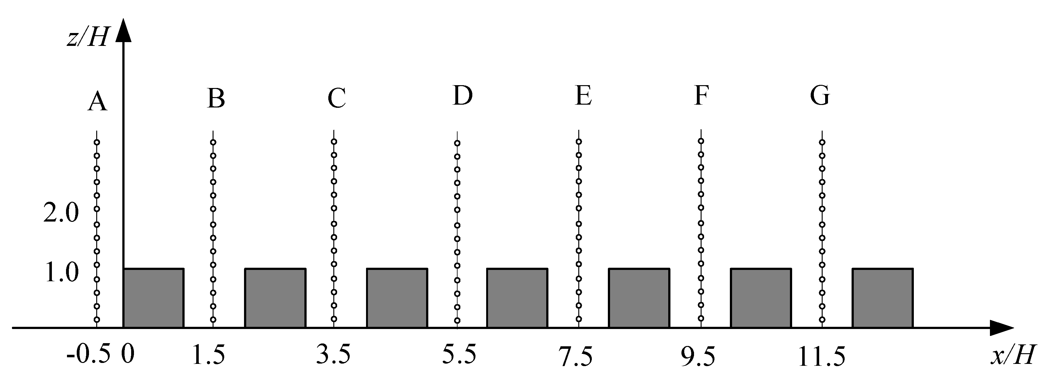
To obtain the factors influencing the drag coefficient for a standard building, a numerical simulation was conducted based on the wind tunnel tests reported by Brown [28]. The specific size of the wind tunnel was 18.3 × 3.7 × 2.1 m (L × W × H), and the cubes comprised 11 × 7 neatly arranged wood cubes. The size of each cube was 0.15 m in each dimension (L = W = H); λ f is the cube coverage of the computational domain, which was equal to 0.25. The layout of the cubes is shown in Figure 1. The drag coefficient was analyzed for cubes in Row 6, marked with black boxes in Figure 1a.
In the entire computational domain, hexahedral meshes were adopted to ensure high accuracy. To satisfy the requirements of the Architectural Institute of Japan (AIJ) and European Cooperation in the field of Scientific and Technical Research (COST) [29,30], the number of meshes in the three dimensions (length × width × height) was 350 × 240 × 70. The grid system passed the independence test. The meshes near the ground and the cubes were encrypted; the height of the first layer was 0.005 m, and the mesh stretching ratio near the ground surface in the vertical direction was 1.05. The total number of meshes was 5.88 million. All calculations were performed on a workstation with an Intel (R) Xeon (R) Gold 6226R processor, 32 cores, and 128 GB memory, the time step was 0.0001 s, simulate 30 s and the calculation time of single simulation was about 90 h. The boundary conditions of the numerical model were consistent with those of the wind tunnel tests in Brown [28]. The average wind velocity at the inlet can be expressed as follows:
u ¯ i n ( z ) = u ¯ r e f ( z z r e f ) α
where u ¯ r e f is the reference average wind, the reference height z r e f = 0.15   m , and the exponent α = 0.16, the selection of these parameters was based on the wind tunnel test. The commercial software fluent was employed for the simulation, and the standard LES solver was used. Table 1 lists the discretization schemes and solution techniques.
Figure 2 shows the numerical simulation monitored profiles for the cubes in Row 6 (the horizontal direction’s details location as the red points show in Figure 1a). The flow field features such as wind velocity, pressure, TKE, SGS dissipation, and SGS TKE were monitored during the simulation process.

2.3. Results and Validation of the Simulated Wind Field

(1)
Mean wind velocity (U)
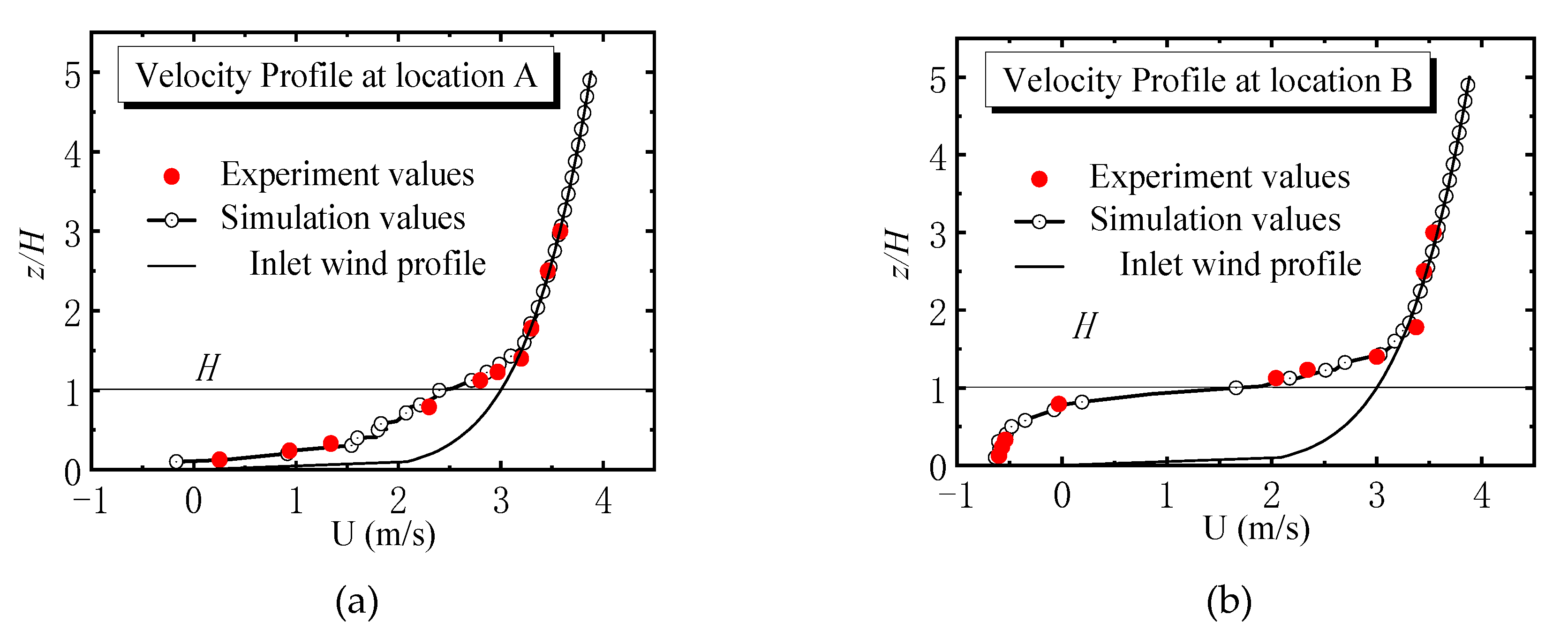
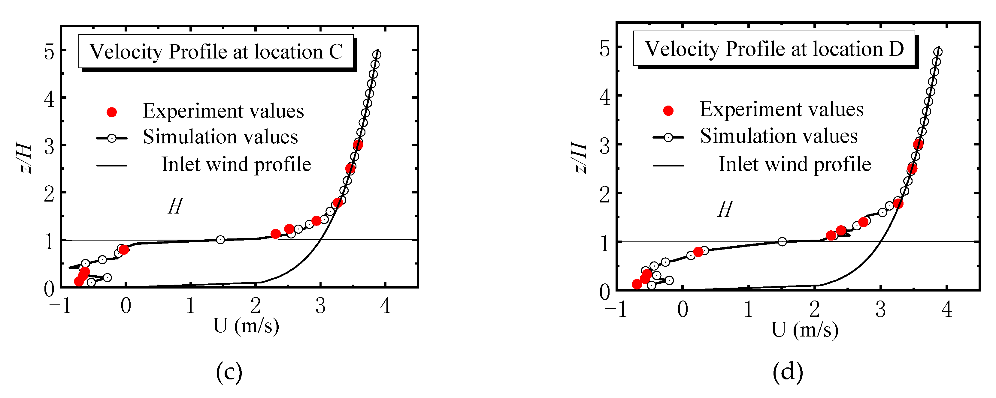
The longitudinal average wind profiles at locations A to D (Figure 2) are shown in Figure 3. The open circles represent the simulation results of the present study and the solid red points represent the measured values from the wind tunnel test performed by Brown et al. [28]. In contrast, the solid black line represents the inlet wind speed profile. Figure 3a shows the comparison of wind profile between the inlet and point A. It was found that the wind velocity at point A was lower than the velocity of the inlet near the ground. However, when z > H, the wind velocity at point A was consistent with the inlet because no building blocks the wind field. Meanwhile, it was also found that the velocity results of the numerical simulations were compatible with the results of the wind tunnel tests, thus validating the numerical simulation. Meanwhile, the mean velocity profiles at locations B and C near the ground demonstrated significant fluctuations in comparison with location A; in particular, negative wind velocities occurred at some points. This scenario occurred because location A is not influenced by the presence of cubes, whereas profiles B to D are heavily affected by cubes. The deviation decreased with increasing height, and the wind velocity became steady when the height was more than twice that of the cubes. The detailed velocity profile graph is shown in Appendix A.
(2)
Turbulent kinetic energy (TKE)
TKE is an essential index for the fluctuation characteristics of wind fields. Especially in the near-surface region of the canopy. Figure 4 shows the average TKE profiles of the simulated model near the ground, where the height H equals 0.15 m. The figures indicate the values of the TKE increase along the horizontal direction. It was relatively small near the ground for points B to E, but the TKE was relatively large near the ground due to the reverse vortex effect for points F and G.
(3)
SGS TKE and SGS dissipation
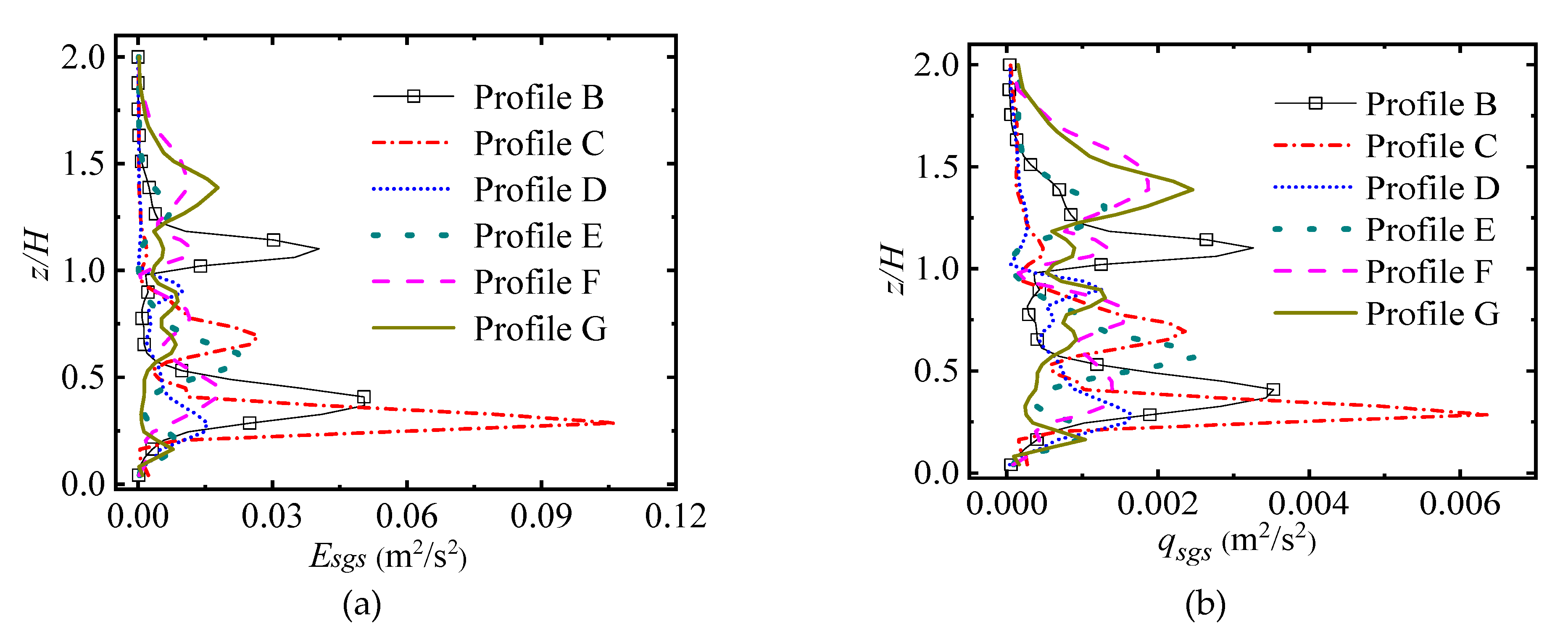
The basic concept of the LES method is to solve the large-scale vortices directly, while the small-scale vortices are closed with the SGS. Thus, the SGS TKE and SGS dissipation are two important components of the energy composition of the flow field in the actual simulation. Considering the effects of the sub-grid TKE and sub-grid dissipation allows the drag coefficient near the ground to be analyzed more accurately. Figure 5 shows the SGS TKE and SGS dissipation distributions for profiles B to G.
As shown in Figure 5, the values of the sub-grid TKE were larger than those of the sub-grid dissipation in the overall trend, and the peak value of the SGS dissipation reached 0.006. The SGS kinetic energy and dissipation were relatively large in the first three rows of buildings and tended to be stable from D to G. Generally, the peak value of SGS kinetic energy and dissipation usually appeared at the average building height. Similar studies have been reported in Martilli and Santiago [21]. However, B and C’s peak value appeared at 0.3H, which was mainly due to the grid filtering. Therefore, the effects of the dissipation on the numerical simulation results should be considered for high-precision numerical simulations.

2.4. Proposed Modified Drag Model Procedure

The drag force on the cubes for the vertical and horizontal sections are as shown in Figure 1, where the shaded area represents a canyon unit. In this case, during the procedure when the volume integral of the pressure gradient term was transformed into the integral over the surfaces limiting the volume, an extra term appeared in the momentum equation that involved the integral of the pressure over the surface of the obstacles [21], and can be expressed as:
1 ρ V V P x i d v = 1 ρ V W P n i d W + 1 ρ V i = i , M j = 1 , N W ( i , j ) P n i d W
where V is the air volume, P is the pressure, W is the external surface of the grid cell, W ( i , j ) is the surface area of cube (i, j). The sum is made over all the N and M obstacles present in the grid cell. ρ is the air density, and n i is the scalar for the i direction.
The equations above can be used to integrate an individual cube at different heights to obtain the drag effects of individual cubes. Using the results of the CFD model, this term can be estimated at different heights in the canopy (e.g., for the averaging volumes defined above, see Figure 1) and for each building canyon unit, which can be expressed as follows:
D k = 1 ρ V W c u b e P n x d W = 1 ρ ( x y z k H 2 z k ) × j = j S , j e ( P i s , j , k P i e , j , k ) H N c u b e z k
where P i s , j , k and P i e , j , k are the pressures at the corners of the cubes; js and je represent the corners of cubes in the Y direction, and is and ie represent the corners in the X direction, as shown in Figure 1. N c u b e represents the number of grid points divided by the cubes ( N c u b e = j e j s + 1 ) .
Assuming Δx = Δy = 2H in each region, Equation (8) can be simplified as follows:
D k = 1 ρ V W c u b e P n i d S = 1 r 3 H N c u b e j = j s , j e ( P i s , j , k - P i e , j , k )
The drag coefficients can be also expressed as
D k = α k c d U K | U K |
where α k represents the cube density.
α = H z x y z H 2 z = H z 4 H 2 H 2 z = 1 3 H
In Equations (9) and (10),
1 3 H c d U | U | = 1 ρ 3 H N c u b e j = j s , j e ( P i s , j , k P i e , j , k ) .
Therefore,
c d = 1 U | U | 1 ρ N c u b e j = j s , j e ( P i s , j , k P i e , j , k )
c d can also be expressed as follows:
c d = P 1 2 ρ U | U |
where P = j = j s , j e ( P i s , j , k P i e , j , k ) 2 N c u b e .
As shown in Equation (14), the drag coefficient for the specified section is the pressure change over the kinetic energy. According to Equations (7)–(14), this method can simulate the drag coefficient at heights greater than 0.5 times the cube height. However, the velocity near the ground is usually very small, and the drag coefficient obtained by Equation (14) near the ground is large. As a result, negative average wind speeds may occur in several places. Therefore, the drag coefficient model proposed by Coceal et al. [19] cannot be applied in the near-surface region.
Meanwhile, owing to the blockage of the airflow by cubes and obstacles near the ground, the wind field is complex and has high turbulence, and the pressure difference is not only simply caused by the average wind velocity, but also affected by the fluctuating component. Considering turbulence effects such as the AKE, TKE, SGS TKE, and dissipation, Equation (13) can be modified as follows:
C D mod = | U | U | U 2 + v k 2 + v ε S G S 2 + q S G S 2 | 1 ρ N c u b e j = j s , j e ( P i s , j , k P i e , j , k )

2.5. Validation of the Variation in the Drag Coefficient with Height

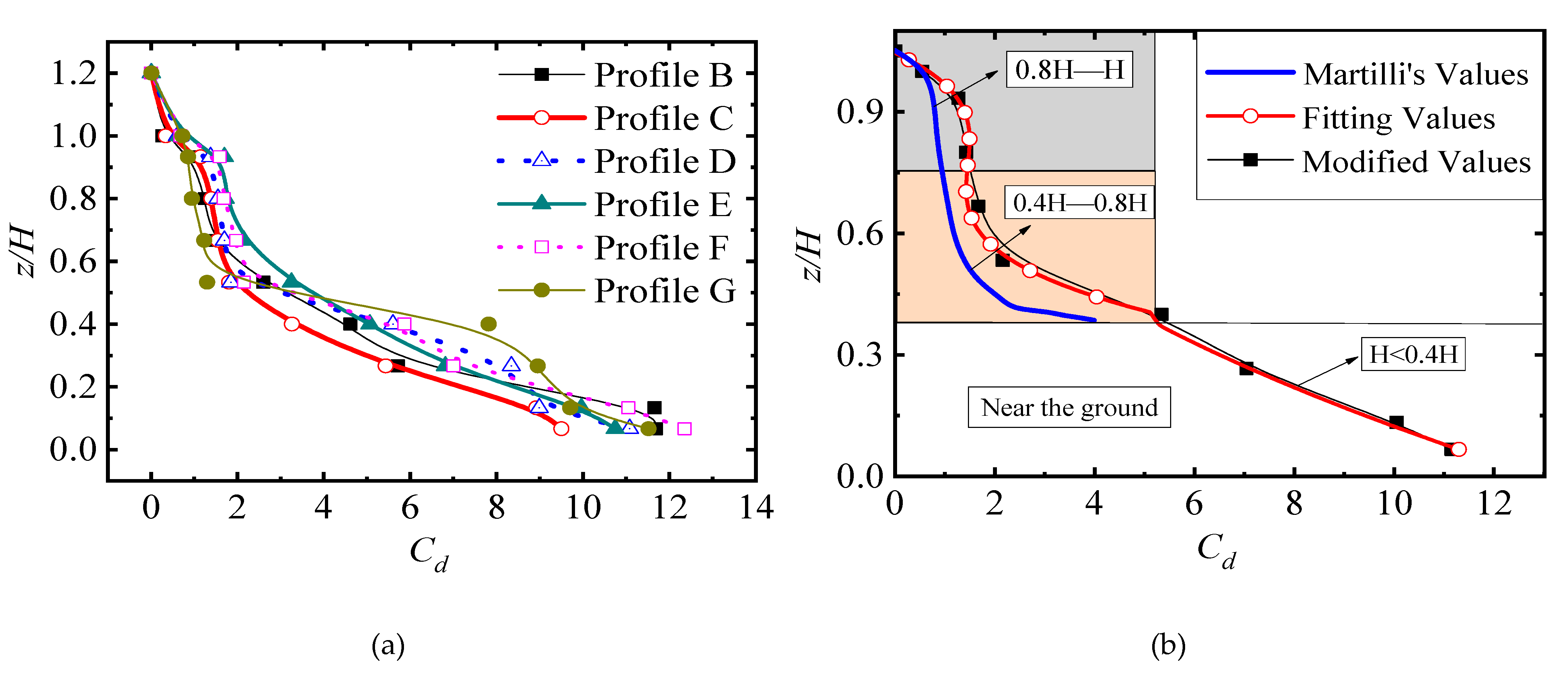
By obtaining the above parameters (the AKE, TKE, SGS TKE, and SGS dissipation), the drag coefficient distribution can then be determined using Equation (15). Figure 6a shows the drag coefficient distribution for profiles B to G, revealing that the drag coefficient relatively large near the ground, and it decreases with the increase of height. Compared with previous studies, considering the TKE and SGS dissipation with the method in this study allows the distribution of the drag coefficient to be obtained at lower positions. Figure 6b shows the average drag coefficient for profiles B to G; the results reported by Martilli and Santiago [21] are also presented. In Figure 6b, it is worth noting that the drag coefficients obtained with the proposed model at positions above 0.8 times the cube height, i.e., 0.8H, agree well with Martilli’s results. However, at heights of 0.4H to 0.8H, the drag coefficients deviate from Martilli’s results. In particular, at positions below 0.4 times the cube height, no results were provided by Martilli. The drag coefficient along the height can be fitted as polynomial functions as follows:
c d ( z ) = 12.87 z 2 25.25 z + 12.92 ,   0 < z < 0.4
c d ( z ) = 81.58 z 3 + 188.56 z 2 144.4 z + 38.1 ,   0.4 < z < 1.2
where z = Z/H, 0 < z < 1.2. It should be noted that when z is greater than 1.2, the drag effects are very small and c d can be considered as equal to 0.
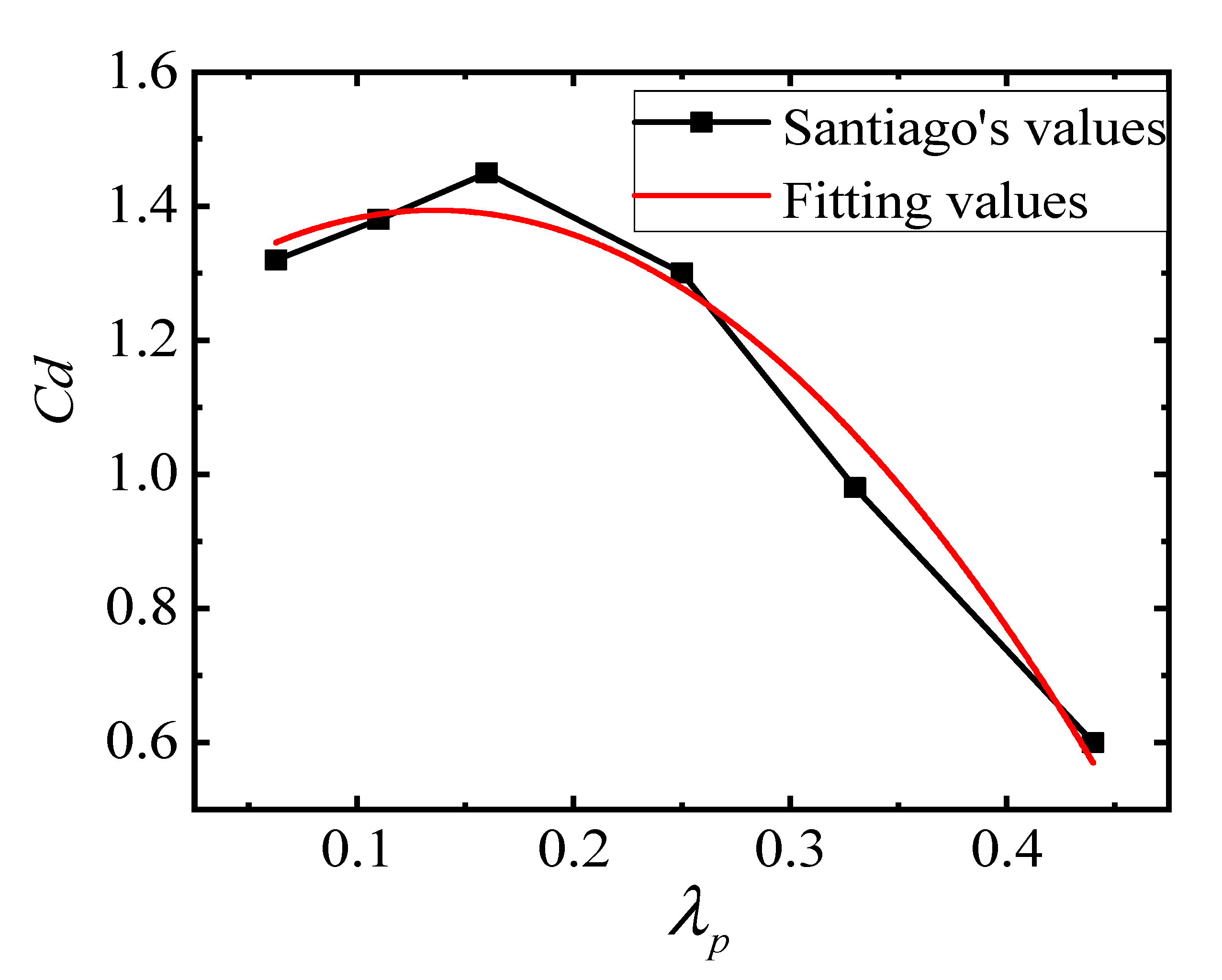
The drag coefficient distribution given by Equation (16) can also be influenced by λ p in the actual urban canopy layer. To address this problem, different cube densities obtained by Santiago et al. [23] are fitted as polynomial functions to define parameter γ , as shown in Figure 7. The fitted parameter, γ , is expressed as follows:
γ = 8.9 λ p 2 + 2.42 λ p + 1.229 ,   0.5 < λ p < 0.45
The drag coefficient for the urban canopy considering the height and density of cubes can be finally expressed as follows:
c d ( z , λ ) = γ c d ( z ) ,   0 < z < 1.2

3. Case Study

The Meixi Lake International Community [31] was considered as a case study. The Meixi Lake community is in the west of Changsha, China, and is referred to as the “National Green Low-Carbon Demonstration New Zone” and “Changsha New City Center”. The planned population of this community is approximately 4,000,000, thereby forming a densely populated area. Therefore, selecting the Meixi Lake community as a case study is of practical importance for assessment of the wind environment.

3.1. Calculation Models and Meshes

The terrain data in the CFD simulations were obtained using the Geospatial Data Cloud and further processed using Global Mapper [32]. The elevation information of the mountain terrain model was processed through the format transformation of the geospatial data. The building model information was from the Arc map. The size of the computational domain was 10 km (length) × 9 km (width) × 3 km (height), as shown in Figure 8.
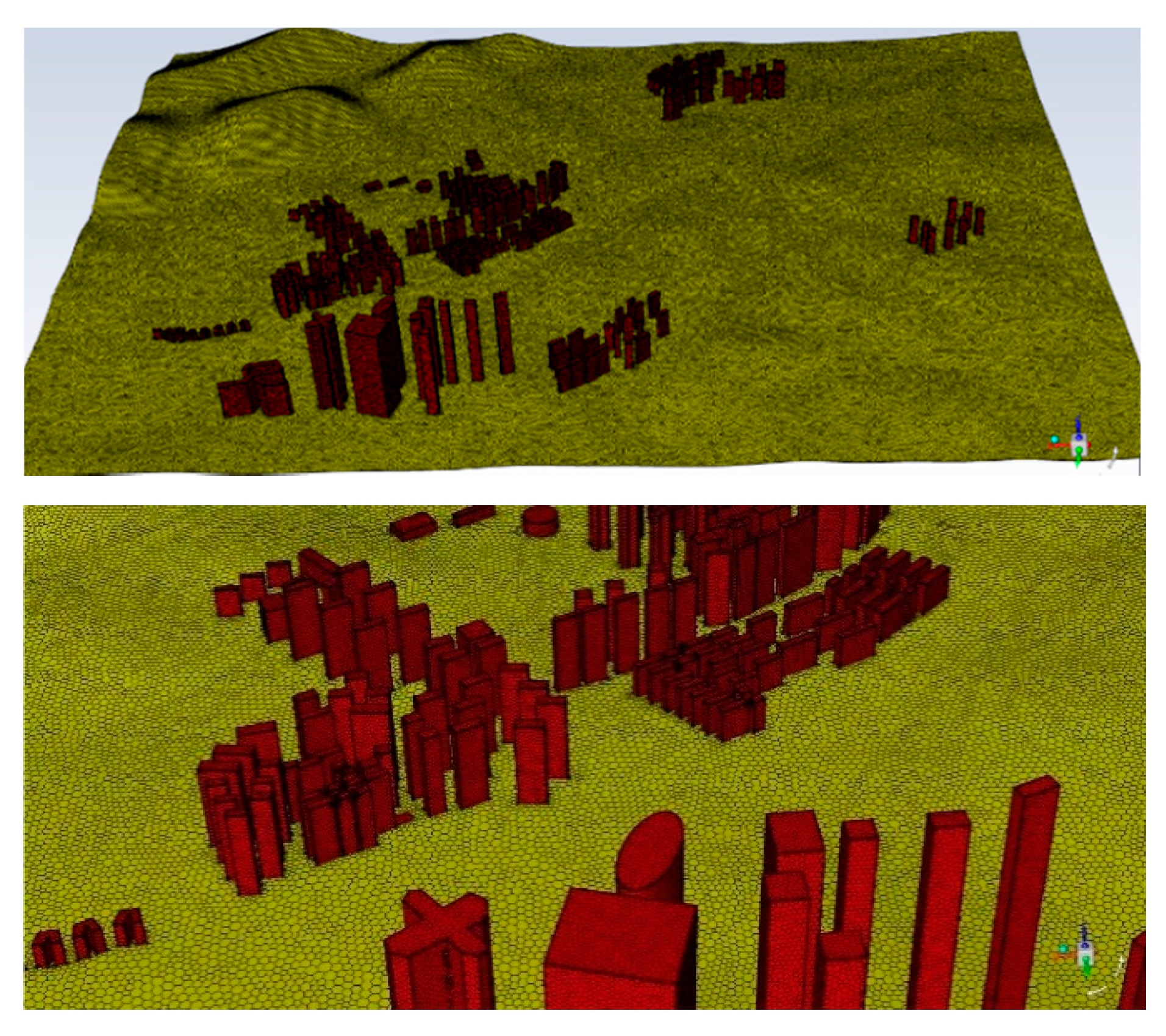
Tetrahedral and polyhedron meshes were employed for the numerical simulation. The grids near the ground and the buildings were refined, and the total number of tetrahedral meshes for the entire computation domain was 2,565,4861, while the number of polyhedral meshes of the same size was 1,416,5854. Considering the computing efficiency and computing resources, the polyhedral meshes were arranged in the computational domain as shown in Figure 9. All calculations were performed on a workstation with an Intel (R) Xeon (R) Gold 6226R processor, 32 cores, and 128 GB memory, the time step was 0.001 s, simulate 10 s, and the calculation time of single simulation was about 20 h. The SGS model provided by the dynamic Smagorinsky-Lilly Equation [33] was used to account for the turbulence. The discretization schemes and solution techniques were the same as those presented in Table 1.

3.2. Mesoscale Coupling Wind Profile and Wind Velocity Profile Parameters

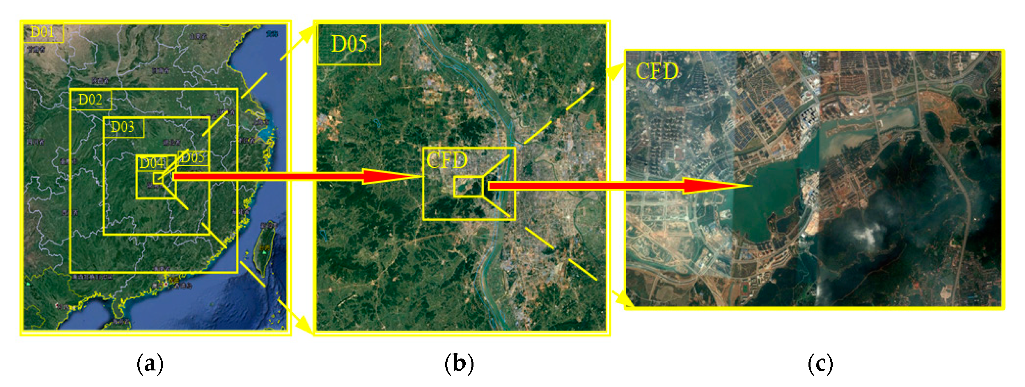
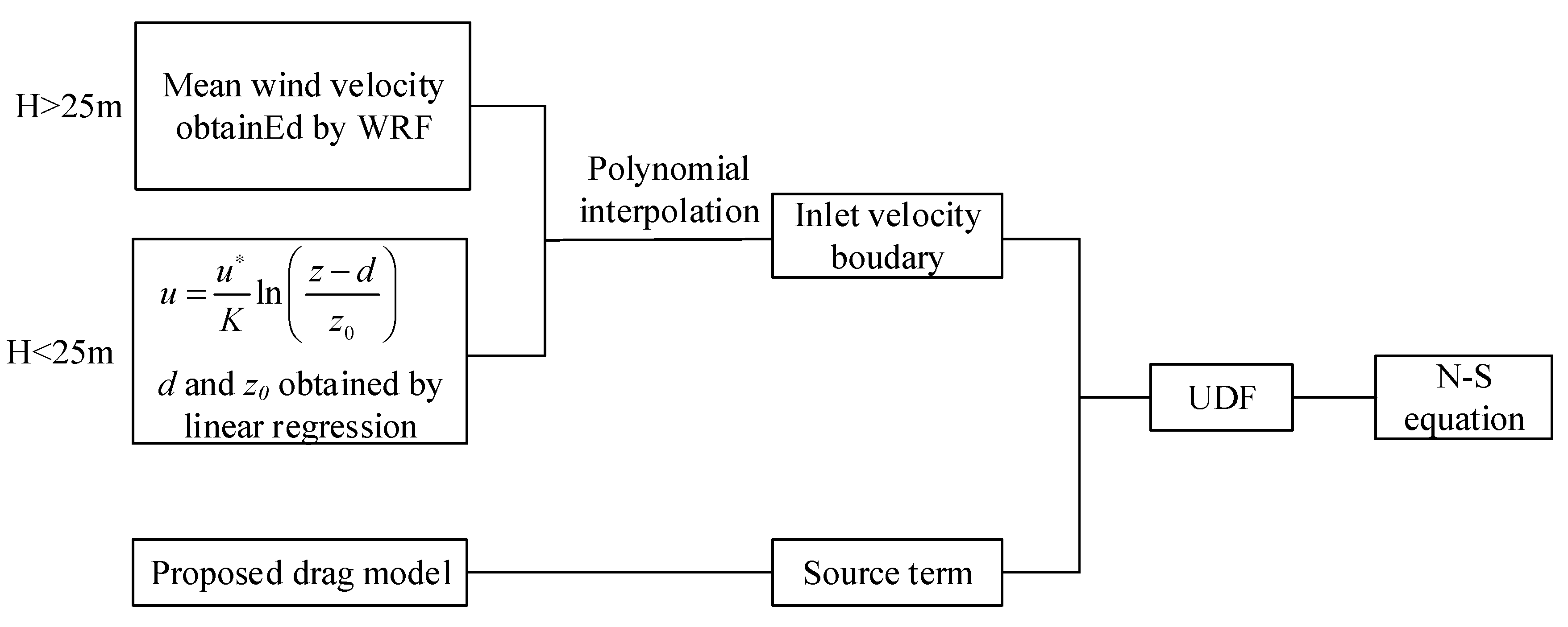
A multi-scale coupling technique [32] combining weather research forecasting (WRF) and computational fluid dynamics (CFD) was used to obtain the wind inlet boundary. Figure 10 shows the coupling flow chart, the detailed set-up of the WRF-CFD coupling is shown in Appendix B.
The average wind velocity for the numerical simulation of the urban canopy can be obtained through the coupling of the WRF and CFD approaches. However, the first WRF layer was 25 m in height, and velocity values below 25 m could not be captured. However, in the CFD model, a surface with a height of 25 m was important in the UABL. A logarithmic wind profile equation was used to describe the wind field near the ground, as follows: z0
u = u K ln ( z d z 0 )
where u is the average wind velocity, u is the surface friction velocity, K is the von Karman constant (K = 0.4), z 0 is the surface roughness height, and d is the height of the zero plane.
According to the Macdonald equation [34], the displacement height, d, of the actual urban canopy can be expressed as follows:
d H max = c 0 X 2 + ( a 0 λ p b 0 c 0 ) X
X = σ H + H a v e H max , 0 X 1.0
where a 0 , b 0 , and c 0 are regression parameters with values of 1.29, 0.36, and −0.17, respectively; σ H Standard deviation of the building height. X is defined as the ratio of the part above the average height ( H a v e + σ H ) to the maximum height ( H max ).
In accordance with the Macdonald equation, the correction equation for z 0 (the roughness height of the urban canopy) can be expressed as follows:
z 0 z 0 ( m a c ) = b 1 Y 2 + c 1 Y + a 1
where Y = λ P σ H H a v e , and b 1 , c 1 , and a 1 are regression parameters with values of 0.71, 20.21, and −0.77, respectively; z 0 ( m a c ) is the roughness height calculated using the Macdonald equation [34].
Based on the above equations, parameters d and z 0 ( m a c ) can be quantified as having values of 8.8 and 1.53 m, respectively, by considering the amended nonlinear regression method. Based on the logarithmic interpolation method, the wind velocity profile can be expressed as follows:
u = u K ln ( z 8.8 1.53 )
where u = 0.23   m / s .
The wind velocity field above 25 m was provided by the WRF, while the polynomial interpolation method [33] was adopted for the wind field below 25 m. By combining these two wind fields, the inlet wind velocity boundary could thus be determined.

3.3. Drag Model Parameters

According to the planning map of Meixi Lake community and the urban database proposed by Kanda [24] (http://www.ide.titech.ac.jp/~kandalab/download/LES_URBAN/index.html), it was found that the average height of the study area was approximately 25 m, and the maximum height of the buildings was 240 m. Therefore, σ H is 15 m, λ f and λ p are taken as 0.34 and 0.17, respectively, and c d can be expressed as follows:
c d ( z ) = γ ( 12.87 z 2 25.25 z + 12 . 92 )
γ = 5.6 λ p 2 + 1.31 λ p + 1.01
L c = 2 40 ( 1 0.17 ) 0.34 C d ( z ) = 195.3 c d ( z )
Thus, the expression for the drag force is D i = c d ( z ) | U | U i 195.3 . The source terms of the N–S equation are modified using the UDF script, and the drag force was then assigned to the governing equations for the LES, the input flow chart of UDF is shown in Figure 11.

3.4. Results and Discussion

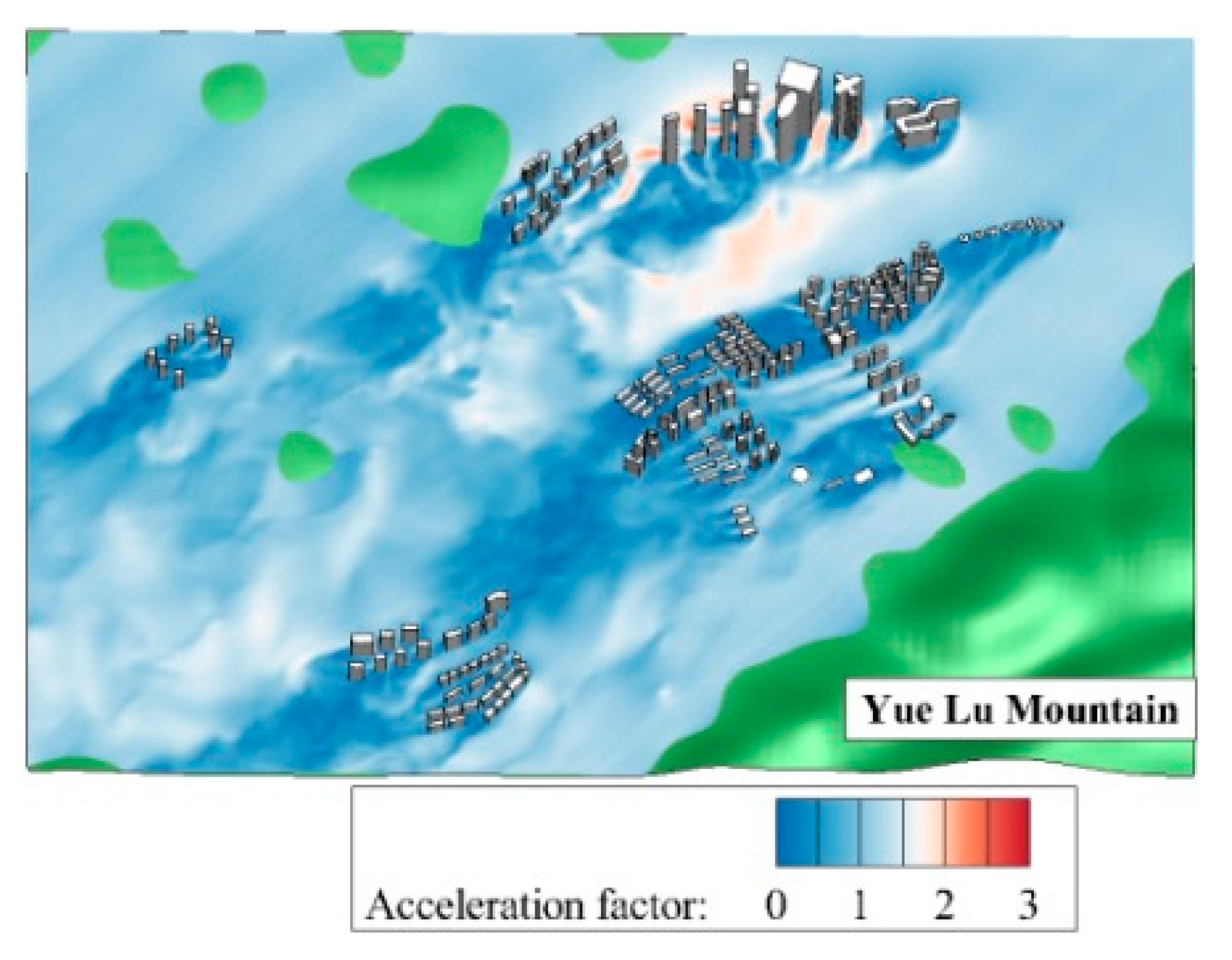
Three cases were considered in the numerical simulation to verify the accuracy of the proposed canopy resistance model. In Cases 1 and 2, the drag effect was considered in the N–S equation by adding corresponding source terms; the proposed method was utilized in Case 1, while in Case 2, a constant drag coefficient of 3.0 was employed according to the method described in Belcher et al. [35]. However, in Case 3, no drag effect was considered. Except for the source terms, the other boundary conditions and calculation parameters were identical for Cases 1 to 3. The acceleration factor contour of Case 1 is shown in Figure 12.
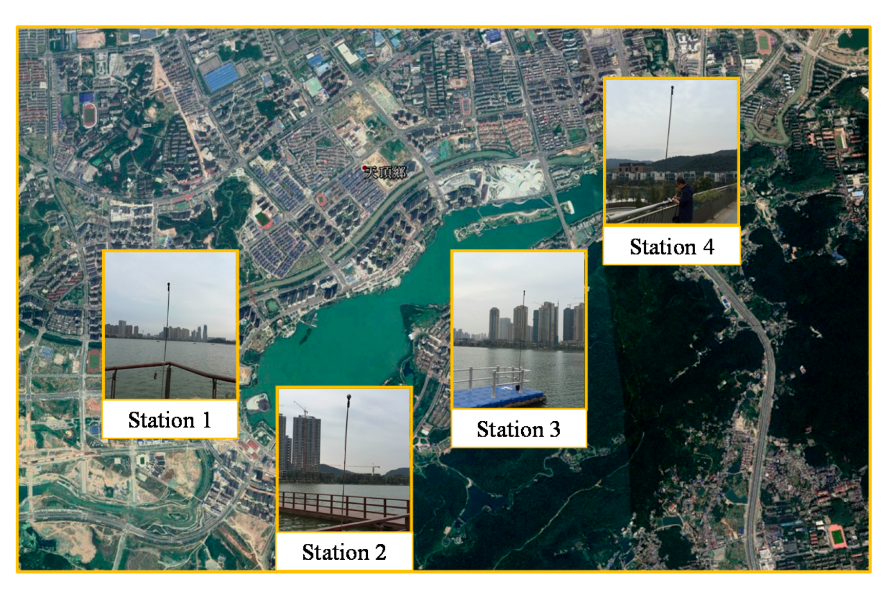
Four handheld anemometers (XM-AS8336) were installed at the Meixi Lake community to monitor the real-time wind field data on the day selected for the numerical simulation. The accuracy of the anemometers was 0.1 m/s, and their positions are shown in Figure 13.
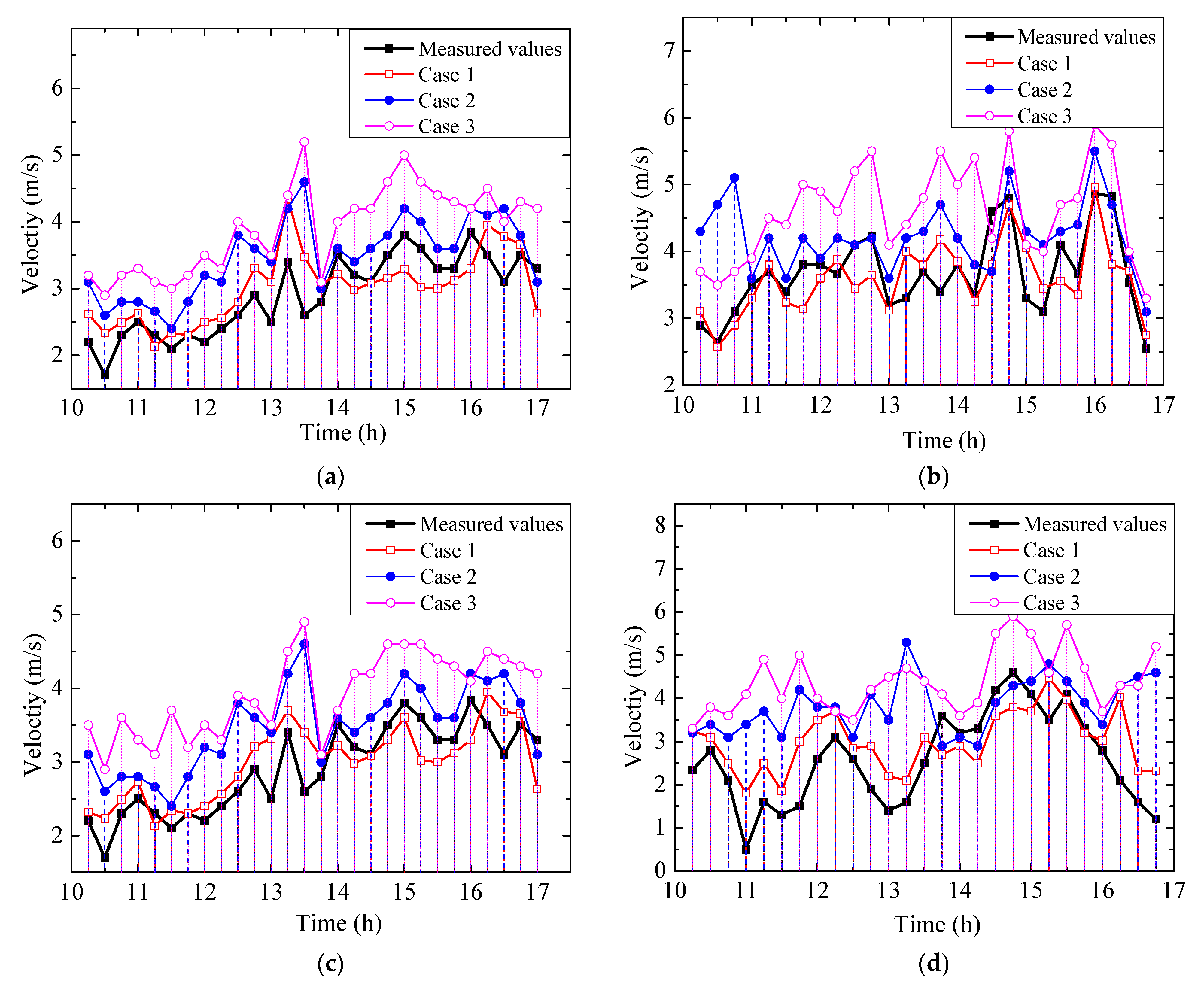
The time-history of the wind velocity at the four stations was obtained from the anemometers, and the wind velocity data were averaged hourly. Station 1 was a sightseeing park, Station 2 was an events plaza, Station 3 was a business mall, and Station 4 was a middle school. Figure 14 shows comparisons between the field measurement and numerical simulation results. It is noteworthy that the simulation results for the wind velocity time-history obtained using the proposed drag model (Case 1) agree well with the field measurement values, whereas the case without consideration of the drag coefficient (Case 3) results in large discrepancies with the field measurements.
Based on the mean wind velocity, the performance of the different methods can be evaluated at a macro level. Table 2 summarizes the comparison of the time-averaged mean velocities (from 10:00–17:00) between the field measurements and numerical simulations. The mean velocities obtained using the proposed method (Case 1) were close to the field-measured values for Stations 1–4. However, the mean velocity values obtained using the other two methods were greater than the measured values.
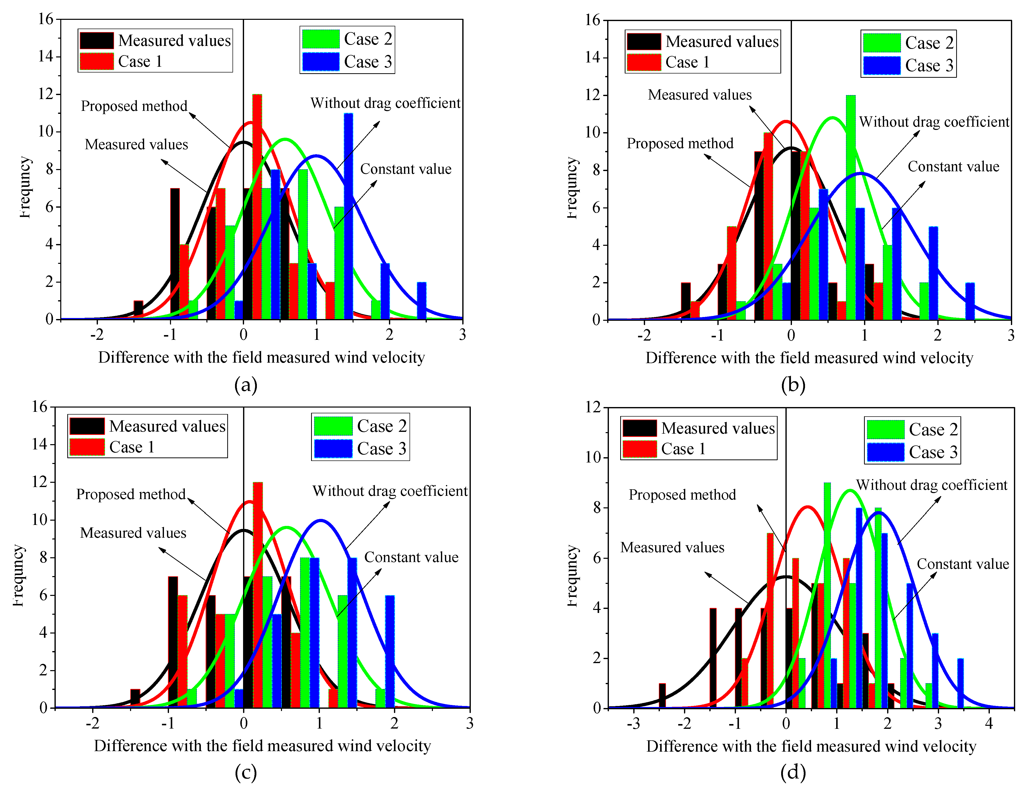
In Figure 15, histograms showing the measured values and different case simulation values are analyzed. The mean value and the standard deviation in Figure 15 can represent the speed deviation and discrete for each case. Using the measured wind speed as the reference value (vertical line in Figure 15), it is clear that the mean velocity values of the proposed method were in better agreement with the field-measured values than the mean values obtained with the other two methods, indicating the superiority of the proposed method. Stations 1 and 3 were located in the lake, where the wind field was not blocked by buildings or mountains; hence, the standard deviation for the different cases maintained the same level. However, because the wind fields at Stations 2 and 4 were affected by buildings and obstacles, the standard deviations of Cases 2 and 3 exhibited some deviations from the measured values.

4. Conclusions

Previous studies about the drag coefficient on the fluid in urban canopy usually consider the mean wind. The drag coefficient models are not sufficiently straightforward for application in practical engineering. Drag coefficient models that do not consider the turbulence component cannot be adapted for simulating the wind field features near the ground surface. However, the drag coefficient near the ground has an essential impact on the pedestrian level wind environment. In this study, a novel canopy drag model was proposed to amend the drag coefficient for a typical urban canopy at various heights based on the LES. The effects of factors in the LES, such as the AKE, TKE, SGS dissipation, and SGS TKE, were considered to amend the drag coefficient variations with building height, and drag coefficient equations for the urban canopy were presented considering the height and density of buildings. Meanwhile, the multi-scale coupling wind velocity boundary was utilized to obtain the inlet boundary and obtained the detailed wind field distribution of the Meixi Lake community. The findings are summarized as follows:
(1)
The mean velocity profiles near the ground demonstrate significant fluctuations. When the height is more than twice that of the buildings, the wind profile is consistent with the inlet profile. The maximum value of TKE usually appears near the height of 1.2H. High-precision numerical simulations should consider the effects of the SGS TKE and SGS dissipation on the numerical simulation.
(2)
Compared with the current studies, the drag coefficient at positions below 0.4 times of building height was obtained. The result shows that the drag coefficient is relatively large near the ground and decreases with the increase in height. The decay rate of drag coefficient below 0.4H is significantly higher than the height greater than 0.4H.
(3)
The numerical simulation considered three types of drag models (e.g., the proposed method, Belcher’s method, and no drag effect), comparing the mean values and standard deviations with the measured velocities. It found that the proposed model simulation results were in good agreement with the measured values. Belcher’s method’s accuracy was second-best, while that of the model with no drag effect was the worst.
In the present study, the drag coefficient distribution varied with the height and the isotropic surface condition was employed in the wind environment simulation. However, the actual urban canopy is anisotropic due to the complex earth surface. Thus, future research will consider the anisotropic parameters of complex surfaces and further improve the simulation accuracy of the urban canopy wind field.

Author Contributions

Conceptualization, L.S. and Y.H.; methodology, L.S.; software, L.S.; validation, L.S., Y.Y.; formal analysis, L.S..; investigation, C.C.; resources, L.S.; data curation, L.S.; writing—original draft preparation, G.X.; writing—review and editing, C.C. and X.H.; visualization, L.S.; supervision, Y.H.; project administration, Y.Y.; funding acquisition, L.S. and Y.H. All authors have read and agreed to the published version of the manuscript.

Funding

The authors acknowledge support by the National Natural Science Foundations of China (51808059). China Postdoctoral Science Foundation (2018M642975). Training Program for Excellent Young Innovators of Changsha (kq1905005). This research was also funded by Natural Science Foundation and Education Project of Hunan Province 2019JJ50688 and 2018JJ1027, and 19B054.

Institutional Review Board Statement

Not applicable

Informed Consent Statement

Not applicable

Data Availability Statement

Data available on request due to restrictions eg privacy or ethical.

Conflicts of Interest

The authors declare no conflict of interest.

Nomenclature

U ( z ) mean wind velocity at the height of z
U0mean wind velocity at the height of h
h0reference height
α power law exponent
u shear velocity of the flow
z0roughness height
Δttime step
AKEaverage kinetic energy
SGSsub-grid scale
TKEturbulent kinetic energy
KVon Kármán constant
dsize of grids near the ground
ε S G S sub-grid scale dissipation
q S G S sub-grid scale turbulent kinetic energy
u ¯ r e f reference average wind
z r e f the reference height
Hheight of the building model
D ¯ i drag force
L c canopy drag length scale
c d ( z ) drag coefficient drag at the height of z
A f average frontal area
β fractional volume
Ppressure
Wouter surface area of the buildings
W ( i , j ) first surface area of cube (i, j)
n i the scalar for the i direction
P i s , j , k the pressures at the corners of the cubes
js, jethe corners of cubes in the Y direction
is, iethe corners in the X direction
α k cube density
N c u b e number of grid points divided by the cubes
λ p building density
λ f frontal area density
γ fitted parameters
Xthe ratio of average height to the maximum height
H max the maximum building height
a, b, cregression parameters
z 0 ( m a c ) Macdonald roughness height
σ H standard deviation of the building height

Appendix A

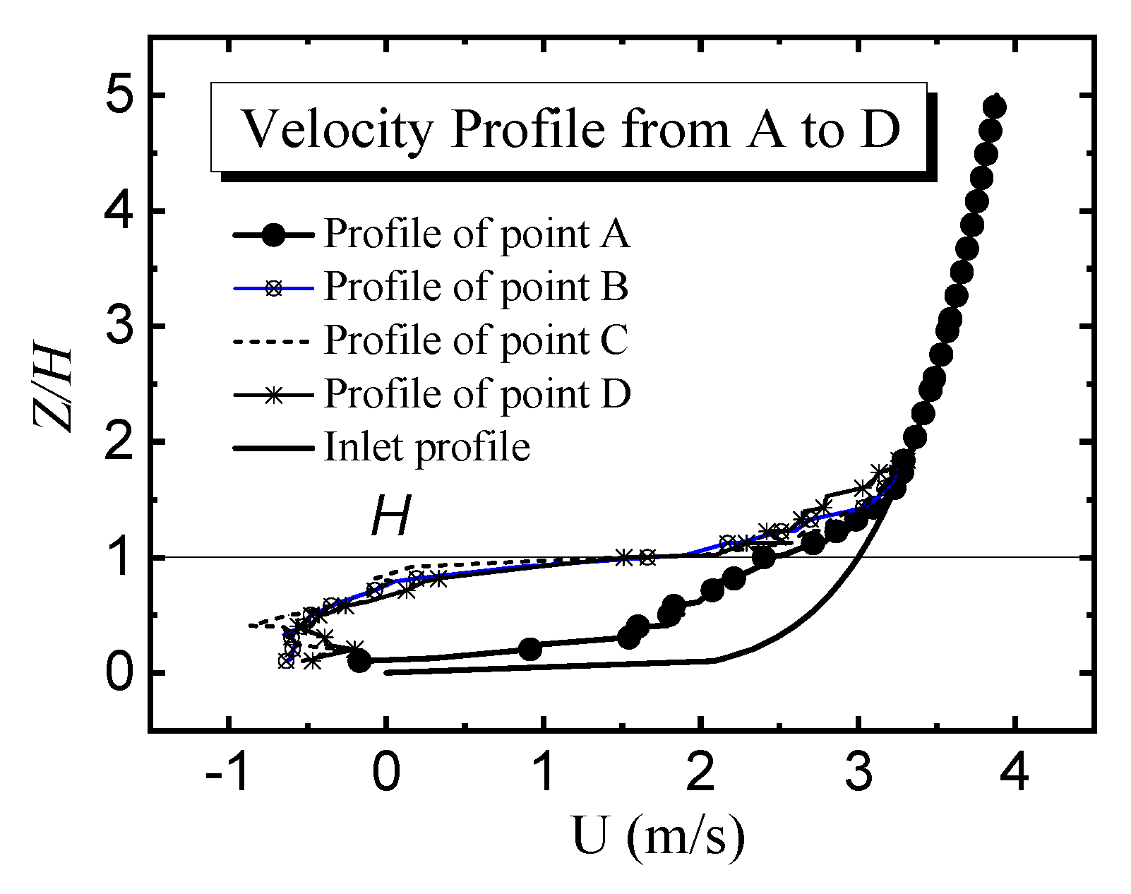
Figure A1. Velocity profiles from A to D.
Energies 14 00796 g0a1
The combined velocity profile of A-Dare shown in Figure A1. It shows that the wind velocity near the ground was lower than the inlet velocity, indicating that the buildings have an obvious blocking effect on the wind field. It also found that the wind velocity at points A to D changed very little. It shows that the wind field tends to be stable after several buildings. Meanwhile, both profiles were fitted by a logarithmic form of Equation (18), and the fitted values are shown in Table A1. The results show the Zref and α increased with the distance and then tends to be stable after passing several buildings.
Table A1. Fitted values.
LocationzrefαAdj. R-Square
Inlet0.150.16100%
Point A0.280.340.897
Point B0.380.670.75
Point C0.380.680.73
Point D0.390.6620.77

Appendix B

Table A2. Nesting information of the five grids/domains.
DomainGrid NumbersGrid Span (km)Size (km × km)Time Step (s)Layer Numbers
15040.52025 × 202524350
29113.51228.5 × 1228.58150
31614.5724.5 × 724.52750
41811.5271.5 × 271.5950
51010.550 × 50350
Note: Grid numbers, grid span, and size are the parameters for horizon direction meshes; layer numbers represent the vertical direction meshes.

References

  1. United Nations Publications. World Urbanization Prospects. 2014: Highlights; United Nations Publications: New York, NY, USA, 2014. [Google Scholar]
  2. Grimmond, C.S.B.; Salmond, J.A.; Oke, T.R.; Offerle, B.; Lemonsu, A. Flux and turbulence measurements at a densely built-up site in Marseille: Heat, mass (water and carbon dioxide), and momentum. J. Geophys. Res. Space Phys. 2004, 109, D24101. [Google Scholar] [CrossRef]
  3. Blocken, B.; Stathopoulos, T.; Van Beeck, J. Pedestrian-level wind conditions around buildings: Review of wind-tunnel and CFD techniques and their accuracy for wind comfort assessment. Build. Environ. 2016, 100, 50–81. [Google Scholar] [CrossRef]
  4. Du, Y.; Mak, C.M.; Kwok, K.; Tse, K.-T.; Lee, T.-C.; Ai, Z.; Liu, J.; Niu, J. New criteria for assessing low wind environment at pedestrian level in Hong Kong. Build. Environ. 2017, 123, 23–36. [Google Scholar] [CrossRef] [Green Version]
  5. Kent, C.W.; Grimmond, S.; Barlow, J.; Gatey, D.; Kotthaus, S.; Lindberg, F.; Halios, C.H. Evaluation of urban local-scale aerodynamic parameters: Implications for the vertical profile of wind speed and for source areas. Bound. Layer Meteorol. 2017, 164, 183–213. [Google Scholar] [CrossRef]
  6. Barlow, J.F. Progress in observing and modelling the urban boundary layer. Urban Clim. 2014, 10, 216–240. [Google Scholar] [CrossRef] [Green Version]
  7. Zhu, X.; Iungo, G.V.; Leonardi, S.; Anderson, W. Parametric study of urban-like topographic statistical moments relevant to a priori modeling of bulk aerodynamic parameters. Bound. Layer Meteorol. 2016, 162, 231–253. [Google Scholar] [CrossRef]
  8. Sadique, J.; Yang, X.I.A.; Meneveau, C.; Mittal, R. Aerodynamic Properties of Rough Surfaces with High Aspect-Ratio Roughness Elements: Effect of Aspect Ratio and Arrangements. Bound. Layer Meteorol. 2017, 163, 203–224. [Google Scholar] [CrossRef]
  9. Britter, R.E.; Hanna, S.R. Flow and dispersion in urban areas. Fluid Mech. 2003, 35, 469–496. [Google Scholar] [CrossRef]
  10. Du, Y.; Mak, C.M.; Li, Y. Application of a multi-variable optimization method to determine lift-up design for optimum wind comfort. Build. Environ. 2018, 131, 242–254. [Google Scholar] [CrossRef]
  11. Baik, J.J.; Park, S.B.; Kim, J.J. Urban flow and dispersion simulation using a CFD model coupled to a mesoscale model. J. Appl. Meteorol. Climatol. 2009, 48, 1667–1681. [Google Scholar] [CrossRef]
  12. Kong, L.; Lau, K.K.-L.; Yuan, C.; Chen, Y.; Xu, Y.; Ren, C.; Ng, E. Regulation of outdoor thermal comfort by trees in Hong Kong. Sustain. Cities Soc. 2017, 31, 12–25. [Google Scholar] [CrossRef]
  13. Blocken, B.; Stathopoulos, T.; Carmeliet, J. CFD simulation of the atmospheric boundary layer: Wall function problems. Atmos. Environ. 2007, 41, 238–252. [Google Scholar] [CrossRef]
  14. Blocken, B.; Gualtieri, C. Ten iterative steps for model development and evaluation applied to Computational Fluid Dynamics for Environmental Fluid Mechanics. Environ. Model. Softw. 2012, 33, 1–22. [Google Scholar] [CrossRef]
  15. Blocken, B.; Janssen, W.; Van Hooff, T. CFD simulation for pedestrian wind comfort and wind safety in urban areas: General decision framework and case study for the Eindhoven University campus. Environ. Model. Softw. 2012, 30, 15–34. [Google Scholar] [CrossRef]
  16. Cheng, H.; Castro, I.P. Near Wall Flow over Urban-like Roughness. Bound. Layer Meteorol. 2002, 104, 229–259. [Google Scholar] [CrossRef]
  17. Hagishima, A.; Tanimoto, J. Investigations of urban surface conditions for urban canopy model. Build. Environ. 2005, 40, 1638–1650. [Google Scholar] [CrossRef]
  18. Hagishima, A.; Tanimoto, J.; Nagayama, K.; Meno, S. Aerodynamic Parameters of Regular Arrays of Rectangular Blocks with Various Geometries. Bound. Layer Meteorol. 2009, 132, 315–337. [Google Scholar] [CrossRef]
  19. Coceal, O.; Thomas, T.G.; Castro, I.P.; Belcher, S.E. Mean Flow and Turbulence Statistics over Groups of Urban-like Cubical Obstacles. Bound. Layer Meteorol. 2006, 121, 491–519. [Google Scholar] [CrossRef]
  20. Coceal, O.; Thomas, T.G.; Belcher, S.E. Spatial Variability of Flow Statistics within Regular Building Arrays. Bound. Layer Meteorol. 2007, 125, 537–552. [Google Scholar] [CrossRef]
  21. Martilli, A.; Santiago, J.L. CFD simulation of airflow over a regular array of cubes. Part II: Analysis of spatial average properties. Bound. Layer Meteorol. 2006, 122, 635–654. [Google Scholar] [CrossRef]
  22. Zhang, N. Numerical Simulation Study of the Wind Environment for Urban Roads along River Based on Porous Medium Model. Ph.D. Thesis, Central South University, Changsha, China, 2005. [Google Scholar]
  23. Santiago, J.L.; Coceal, O.; Martilli, A.; Belcher, S.E. Variation of the Sectional Drag Coefficient of a Group of Buildings with Packing Density. Bound. Layer Meteorol. 2008, 128, 445–457. [Google Scholar] [CrossRef]
  24. Kanda, M.; Inagaki, A.; Miyamoto, T.; Gryschka, M.; Raasch, S. A New Aerodynamic Parametrization for Real Urban Surfaces. Bound. Layer Meteorol. 2013, 148, 357–377. [Google Scholar] [CrossRef]
  25. Lien, F.-S.; Yee, E. Numerical Modelling of the Turbulent Flow Developing Within and Over a 3-D Building Array, Part I: A High-Resolution Reynolds-Averaged Navier—Stokes Approach. Bound. Layer Meteorol. 2004, 112, 427–466. [Google Scholar] [CrossRef]
  26. Wooding, R.A.; Bradley, E.F.; Marshall, J.K. Drag due to regular arrays of roughness elements of varying geometry. Bound. Layer Meteorol. 1973, 5, 285–308. [Google Scholar] [CrossRef]
  27. Coceal, O.; Belcher, S.E. A canopy model of mean winds through urban areas. Q. J. R. Meteorol. Soc. 2004, 130, 1349–1372. [Google Scholar] [CrossRef] [Green Version]
  28. Brown, M.J.; Lawson, R.E.; DeCroix, D.S.; Lee, R.L. Comparison of centerline velocity measurements obtained around 2D and 3D building arrays in a wind tunel. Int. Soc. Environ. Hydraul. Conf. 2001, 4162–4164. Available online: https://www.researchgate.net/publication/236512119_COMPARISON_OF_CENTERLINE_VELOCITY_MEASUREMENTS_OBTAINED_AROUND_2D_AND_3D_BUILDING_ARRAYS_IN_A_WIND_TUNNEL (accessed on 30 December 2020).
  29. Franke, J.; Jensen, C.; Hirsch, A.G.; Krüs, H.W.; Schatzmann, M.; Westbury, P.S.; Miles, S.D.; Wisse, J.A.; Wright, N.G. Recommendations on the use of CFD in wind engineering. In Proceedings of the International Conference on Urban Wind Engineering and Building Aerodynamics, COST Action C14, Impact of wind and Storm on City Life Built Environment, von Karman Institute, Rhode-Saint-Genèse, Belgium, 5–7 May 2004; Academic: Sint-Genesius-Rode, Belgium, 2004. [Google Scholar]
  30. Tominaga, Y.; Mochida, A.; Yoshie, R.; Kataoka, H.; Nozu, T.; Yoshikawa, M.; Shirasawa, T. AIJ guidelines for practical applications of CFD to pedestrian wind environment around buildings. J. Wind. Eng. Ind. Aerodyn. 2008, 96, 1749–1761. [Google Scholar] [CrossRef]
  31. Shen, L.; Han, Y.; Cai, C.S.; Xu, G.; Hua, X. Exceedance Probability Assessment of Pedestrian Wind Environment Based on Multiscale Coupling Numerical Simulation. J. Aerosp. Eng. 2020, 33, 05020002. [Google Scholar] [CrossRef]
  32. Han, Y.; Shen, L.; Xu, G.J.; Cai, C.S.; Dong, G.C.; Zhang, J.R. Multiscale simulation of wind field on a long-span bridge site in mountainous area. J. Wind Eng. Ind. Aerodyn. 2018, 177, 260–274. [Google Scholar] [CrossRef]
  33. Fluent. Fluent User’s Guide: Version: ANSYS 18.0; Fluent: Lebanon, NH, USA, 2018. [Google Scholar]
  34. Macdonald, R.; Griffiths, R.; Hall, D. An improved method for the estimation of surface roughness of obstacle arrays. Atmos. Environ. 1998, 32, 1857–1864. [Google Scholar] [CrossRef]
  35. Belcher, S.E.; Jerram, N.; Hunt, J.C.R. Adjustment of a turbulent boundary layer to a canopy of roughness elements. J. Fluid Mech. 2003, 488, 369–398. [Google Scholar] [CrossRef] [Green Version]
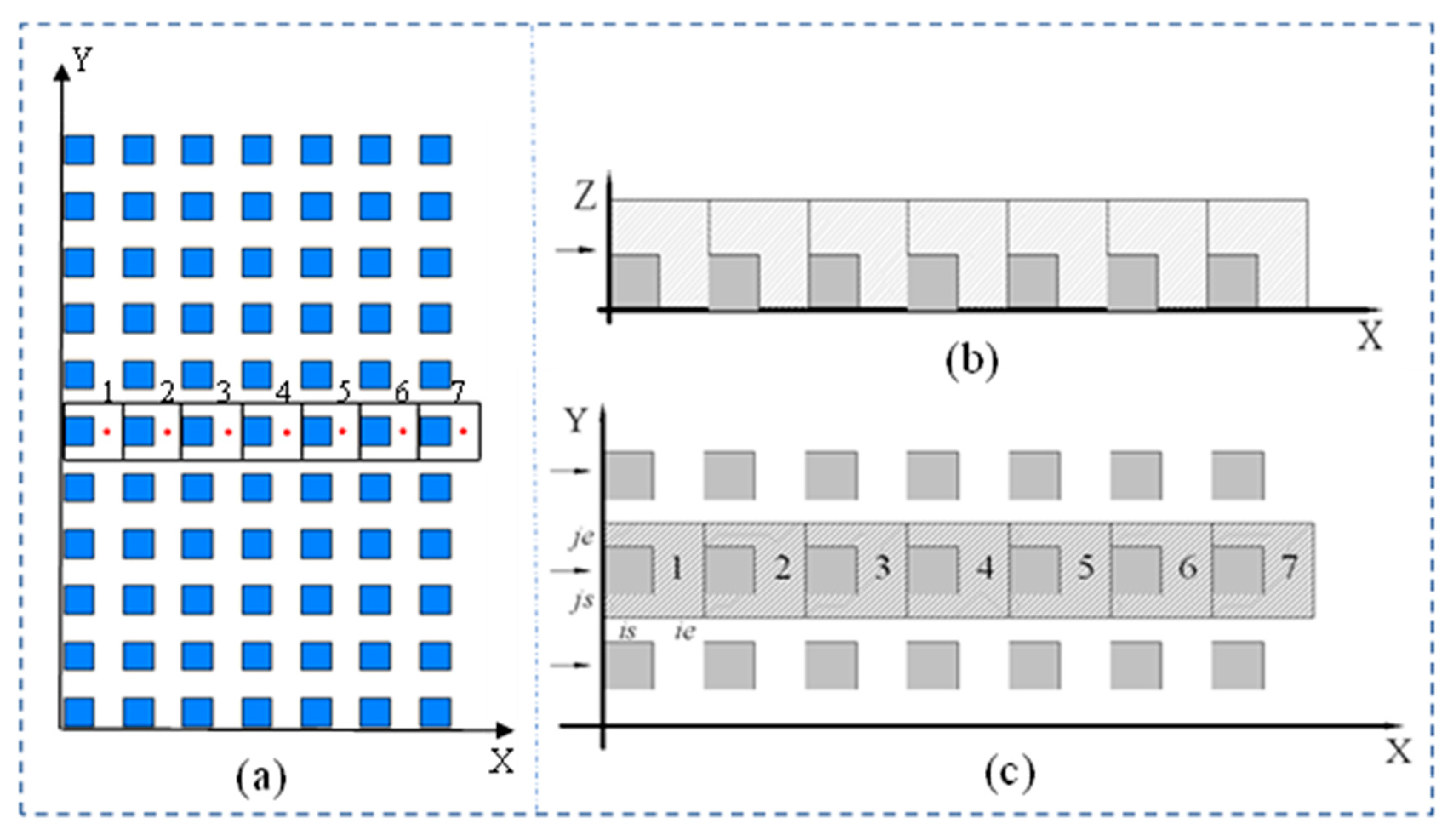
Figure 1. Layout of the cube model. (a) Overall layout of the model; (b) Side view; (c) Plane view.
Energies 14 00796 g001
Figure 2. Monitored profiles in the computational domain.
Energies 14 00796 g002
Figure 3. Longitudinal wind velocity profile distributions at locations A to D. (a) profile at location A; (b) profile at location B; (c) profile at location C; (d) profile at location D.
Energies 14 00796 g003aEnergies 14 00796 g003b
Figure 4. Turbulent kinetic energy results for different profiles.
Energies 14 00796 g004
Figure 5. SGS TKE and SGS dissipation distributions. (a) SGS TKE; (b) SGS dissipation.
Energies 14 00796 g005
Figure 6. Drag coefficient distributions. (a) Drag coefficient distribution for profiles B to G; (b) Comparison of drag coefficient distributions.
Energies 14 00796 g006
Figure 7. Drag coefficients considering different cube densities.
Energies 14 00796 g007
Figure 8. Computational domain (Units: m).
Energies 14 00796 g008
Figure 9. Polyhedral meshes.
Energies 14 00796 g009
Figure 10. Multi-scale coupling diagram. (a) WRF calculation domain (b) WRF calculation domain for D5 (c) CFD calculation domain with building information
Energies 14 00796 g010
Figure 11. The input flow chart of UDF.
Energies 14 00796 g011
Figure 12. Acceleration factor in the horizontal plane in Case 1 (height = 1.5 m, unit: m/s).
Energies 14 00796 g012
Figure 13. Overview of the wind speed monitoring stations.
Energies 14 00796 g013
Figure 14. Comparison of the wind data time-histories for different stations: (a) Station 1, (b) Station 2, (c) Station 3, and (d) Station 4.
Energies 14 00796 g014
Figure 15. Histograms of the wind data time-histories for different stations: (a) Different simulation results vs. field measurement results at Station 1; (b) Different simulation results vs. field measurement results at Station 2; (c) Different simulation results vs. field measurement results at Station 3; (d) Different simulation results vs. field measurement results at Station 4.
Energies 14 00796 g015
Table 1. Discretization schemes and solution techniques.
ParameterType
Time discretizationSecond-order implicit
Pressure discretizationSecond-order upwind
Momentum discretizationBounded central difference
Pressure–velocity couplingPressure-implicit with splitting operators (PISO)
Under relaxation factors0.3 for the pressure and 0.7 for the momentum
Table 2. Mean velocities for different cases.
LocationsMeasured
(m/s)
Proposed Method, Case 1
(m/s)
Constant Drag Coefficient, Case 2
(m/s)
Without Drag Coefficient, Case 3
(m/s)
Station 12.913.013.473.90
Station 23.663.594.234.61
Station 32.912.983.473.93
Station 42.573.003.834.40
Publisher’s Note: MDPI stays neutral with regard to jurisdictional claims in published maps and institutional affiliations.