Modeling of Ultra-Short Term Offshore Wind Power Prediction Based on Condition-Assessment of Wind Turbines

Abstract

More accurate wind power prediction (WPP) is of great significance for the operation of electrical power systems, as offshore wind power penetration increases continuously. As the offshore wind turbines (OWT) are a key system in converting offshore wind power into electrical power, maintaining their condition plays a pivotal role in WPP. However, it is seldom considered in traditional WPP. This paper proposes an ultra-short term offshore WPP methodology based on the condition assessment (CA) of OWTs. Firstly, a modified fuzzy comprehensive evaluation (MFCE) based CA of the OWT is presented with a new defined deterioration of indicators calculated by the relative errors. Long short-term memory (LSTM) neural network is introduced to deal with the complicated interactions between the various monitoring data of an OWT and the dynamic marine environment. Then, with the classifications of the health conditions of the OWT, the historical operation data is classified accordingly. An OWT-condition based WPP with a backpropagation (BP) neural network is developed to deal with the non-linear mapping relations between the numerical weather prediction (NWP) information, health conditions of OWT, and the output power. The results of the case study show the influences of the OWT health conditions to its output power and verifies the effectiveness and higher accuracy of the proposed method.

1. Introduction

Over the decade, there has been an explosive growth of installed offshore wind capacity worldwide. In China, the cumulative installed offshore wind capacity reached 5.93 GW by the end of 2019 and will be about 100 GW by 2030 [1]. While the proportion of offshore wind energy in the electrical power system is becoming more and more significant, ultra-short term offshore wind power prediction (WPP) is now a big concern for the operation of state or regional power grids because of wind power’s volatility and intermittency [2,3,4].

Due to the rapid development of big data and deep learning technologies and no requirement of modeling, research regarding statistical methods and artificial intelligence (AI)-based WPP is now a hotspot. A considerable amount of literature has been published in this area. Generally, it can be summarized into two categories: one is about the method of processing input data [5,6], the other is about the method of improving the performances of algorithms [7,8]. The data for WPP are mainly historical wind power data, historical weather data, numerical weather prediction (NWP) information, etc. Y. Fu et al. assorted the historical wind power data according to the fluctuations and modified the NWP information to alleviate the influences of the heavy wind power fluctuations to the NWP information in offshore WPP [9]. Y.D. Xiong et al. classified and clustered the historical weather data by the improved hierarchical clustering before establishing the short-term WPP model [10]. Data processing is usually for a better computational result with different algorithms. The autoregressive integrated moving average (ARIMA) model is one of the most commonly used statistical prediction methods due to its good performance in time-series forecasting. R. G. Kavasseri et al. proposed a fraction-ARIMA and a f-ARIMA model to forecast wind speed on the day-ahead and two day-ahead horizons [11]. While ARIMA has a certain extent of stability requirement of the input data, the neural network is introduced to modify the prediction results of ARIMA to achieve a higher accuracy [12,13,14]. In order to deal with the poor prediction results for the short-term volatile wind power, a hybrid model combining empirical mode decomposition (EMD) and support vector machine (SVM) was presented in [15]. However, the selection of the kernel function and the SVM parameters are some important factors determining the prediction accuracy [16]. H. Yuan et al. introduced the gravitational search algorithm (GSA) to optimize the kernel function and the parameters of the least squares support vector machine (LSSVM) [17] and they also presented a multi-objective grey wolf optimizer algorithm (MOGWO) to optimize the weights and thresholds of the extreme learning machine (ELM) to improve the stability and accuracy of WPP [18]. With the development of Deep Learning technologies, Q.M. Zhu et al. proposed a multivariate method for ultra-short-term wind power forecasting based on long short-term memory (LSTM) to forecast the ultra-short-term wind power [19]. As the algorithm has its distinct advantages and disadvantages, some works about utilizing hybrid deep learning algorithms were also discussed in [20,21,22,23,24].

However, all of these literatures seldom considered the influences of the health conditions of offshore wind turbines (OWTs) on ultra-short term WPP. The declined health conditions of wind turbines will significantly reduce their capability of wind power generations [25]. R. Byrne et al. and D. Astolfi et al. assessed the wind turbine performance decline with age by analyzed the appropriate operation curves of wind turbine, the result shows that the efficiency reduced about 5% to 6.5% in the 10-year period decline [26,27]. In health condition assessment of wind turbines, several jobs have been done for evaluating the condition variations of the WTs. Based on the monitoring data from SCADA which is produced by Siemens (China) in Shanghai, China, H. Li et al. introduced fuzzy comprehensive evaluation (FCE) to assess the real-time operating conditions of WTs [28]. Y.Q. Xiao et al. proposed a fuzzy prediction model to predict the trend of the predefined parameters, and then a FCE strategy was proposed to evaluate the condition of large-scale WTs. Comparing with [28], the proposed strategy in [29] can demonstrate the condition degradation trend in a timely manner. B.Q. Huang et al. proposed a real-time status evaluation model for OWTs integrating the correlation coefficient method, deterioration analyses, and fuzzy synthetic evaluation [30]. In order to achieve the quantitative relationship between the health condition of WTs and the WPP, M. Yang et al. [31] proposed an ultra-short-term WPP model based on the health condition evaluations with random matrix theory. It is for the onshore WTs. For the OWTs, the marine environment makes the situation very different. As the marine environment is very dynamic (for example, the wind speed at sea is prone to large-scale fluctuations), the operating parameters of OWTs are much easier to have a strong volatility in a short time [32]. In this situation, the most frequently used methods, such as the empirical spectral distribution function in random matrix theory and the deterioration of indicator in FCM, are inapplicable for accurate condition assessment (CA) of OWTs.

To solve the above-mentioned problems, an ultra-short term offshore WPP methodology based on the CA of OWTs is proposed in this paper. Firstly, a modified fuzzy comprehensive evaluation (MFCE) is proposed to assess the conditions of the wind turbines. In MFCE, a system of evaluation is established according to the structure and operation principles of the OWT. The dynamic degradation degree is defined by relative errors which are calculated by the actual value and the predictive value achieve with a LSTM prediction model of the indicator based on marine environment and SCADA data of offshore wind farms. Secondly, an OWT-condition based WPP with backpropagation (BP) neural network is developed to deal with the non-linear mapping relation between the NWP information, health conditions of OWT and the output power. In order to improve the leaning efficiency of the neural network, historical operational data of OWTs will be classified according to the health conditions beforehand. The case study clearly shows the deterioration of OWT affects its energy converting capability and the proposed method demonstrates its effectiveness in dealing with the abrupt condition changes of the OWT and a higher accuracy of offshore WPP.

The main contributions of this paper can be summarized as follows:

(1)

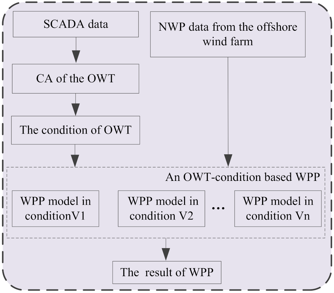
The influences of health condition of the OWT is firstly considered in the ultra-short term offshore WPP. An ultra-short term offshore WPP methodology consisting of CA of the OWT and OWT-condition based WPP is proposed to deal with the relations between NWP information, health condition of the OWT, and output power.

(2)

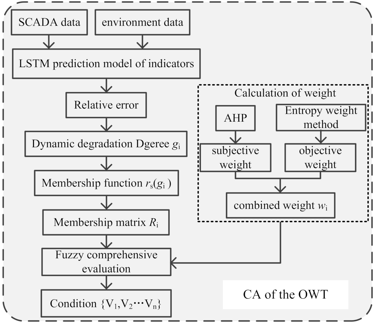
A dynamic deterioration degree is firstly defined to alleviate the influences of the complicated interactions between the various SCADA monitoring data of an OWT and the dynamic marine environment.The dynamic deterioration degrees based MFCE is presented to assess the health conditions of OWTs.

(3)

In order to deal with the influences of the OWT health condition on WPP, data processing based on the classification of historical operational data with conditions of OWTs is proposed to improve the learning efficiency and computing accuracy of the BP neural-network-based WPP.

This paper is organized as follows: the framework of offshore WPP is proposed and explained in Section 2. Section 3 and Section 4 presents CA of the OWT and the OWT-condition based WPP, respectively. Section 5 presents the case study; and Section 6 concludes the paper.

2. Framework of Offshore WPP

Wind energy is absorbed by the wind wheel and transmitted to the generator through the drive chain, and then converted into electrical energy. The whole process can be visually expressed by the power curve. However, the operational data from real projects clearly showed that the real power curve of an OWT is not composed of dots aligned in a line but dispersed dots in a belt [33,34,35,36,37,38]. There are two main reasons for these variations of the output power. One is the big variables of marine environment, such as wind direction, turbulence, air density, etc. The other is the aging and deterioration of the key components in the OWT which may decrease the productivity of the OWT. For ultra-short term WPP, the influences of the environment and the deterioration of the OWT can be treated as two independent variables. In this point, this paper proposes an offshore ultra-short term WPP methodology considering the influences of the condition of the OWTs. It consists of two parts: CA of the OWT based on MFCE, and OWT-condition based WPP. Firstly, CA of the OWT distinguishes the current condition of the OWT from its gradual degradation process. The influences of the deterioration to the capability of energy conversion will be learned by BP neural network from the historical data to deal with the non-linear mapping relation between the NWP information, the health conditions, and the output power. Then, an OWT-condition based model is established to achieve the output power based on the NWP information and the condition of the OWT. The entire procedure is illustrated in Figure 1.

3. CA of OWT

The difficulties in CA of the OWT lie in three aspects: (1) The degradation of the OTW is a gradual process, the boundaries between two adjacent conditions are ambiguous; (2) The harsh marine environment makes the changes of the OWT’s conditions more complicated and more dramatic; (3) While the OWT is a complex multi-component system, the operations of different components in an OWT usually interact with each other, which leads to a correlation between the operational parameters of each component.

FCM is introduced here for its outstanding performances in dealing with the comprehensive influences of multiple uncertain factors. However, in conventional FCE, the criterion for each indicator is based on the variation principles of itself without considering the influences of the dynamic environmental factors and the interactions between different components. It is not quite suitable for the offshore situation. Therefore, an OWT condition assessment model based on MFCE with LSTM neural network is presented here. The main process is illustrated in Figure 2.

3.1. Evaluation System and Condition Categorizes of the OWT

Supposing that there are R_s subsystems determining the capability of OWT electrical power output, and for subsystem s, there are R_si main indicators demonstrating its deterioration process. According to the evaluation system described in [28], R_s can be expanded according to the definition of evaluation system. The evaluation system can be depicted as Figure 3.

According to the production performances and the failure risk of the WT defined in [30], the health conditions of an OWT are defined as four types, which are “V₁”, “V₂”, “V₃”, and “V₄”. The detailed descriptions are presented in

Table 1. Description of each condition.

Health Condition	Description
V1	Excellent operating condition, the equipment is very safe
V2	Good operating condition, relatively safe equipment
V3	The operating status is qualified, the equipment is not safe
V4	Dangerous operation status, high equipment is dangerous

. The OWT in either of these conditions is available but with different productivity and reliability. The condition V₄ is with the lowest productivity and highest failure rate while the condition V₁ is with best productivity and “as good as new”.

3.2. Definition and Calculation of Dynamic Deterioration Degrees

It can be found that during the operation of OWTs, the relative errors between the prediction values and the actual values of the indicator prediction model are small in the normal situation, but large in the abnormal situation [39]. Therefore, instead of the traditional deterioration degrees, a dynamic deterioration degree ε is defined here to demonstrate the dynamic deterioration degrees of the indicators, which is

$${\epsilon }_{\mathrm{i}}=\frac{{\widehat{y}}_{\mathrm{i}}-y_{\mathrm{i}}}{y_{\mathrm{i}}}\times 100\% i=1,2,\dots ,N$$

(1)

In order to simplify the calculations, the dynamic degradation degree of indicator is normalized to (0, 1).

$$g_{\mathrm{i}} =\{\begin{array}{c}{1, \epsilon }_{\mathrm{i}}{ > \epsilon }_{\max }\\ \frac{{\epsilon }_{\mathrm{i}}}{{\epsilon }_{\max }}{, \epsilon }_{\mathrm{i}}{ < \epsilon }_{\max }\end{array}$$

(2)

Considering that LSTM neural network is a kind of deep learning algorithm which has an excellent performance in time series processing and predictions, it is introduced to establish the indicator prediction model based on marine environmental, and SCADA monitoring data here. As a special recurrent neural networks (RNN), LSTM uses a special cell to solve the problem of gradient disappearance and gradient explosion in the training process [19]. The structure of LSTM is shown in Figure 4.

LSTM cell mainly affect the state of the neural network at each moment through three special gates. Specifically, the forget gate is mainly for forgetting the useless information according to the input x_t, the state C_{t − 1} and the output ${\widehat{y}}_{\mathrm{t}-1}$. The input gate is mainly to add new memory from the current input, it determines which part of the information enters the current time C_t according to the input x_t, the state C_{t − 1} and output ${\widehat{y}}_{\mathrm{t}-1}$. Finally, the output gate determines the output ${\widehat{y}}_{\mathrm{t}}$ according to the state C_t, the input x_t, and the output ${\widehat{y}}_{\mathrm{t}-1}$. The implementation formulation is as follows:

$$f_{\mathrm{t}}=\sigma (W_{\mathrm{f}}\times [{\widehat{y}}_{\mathrm{t}-1},x_{\mathrm{t}}]+b_{\mathrm{f}})$$

(3)

$$i_{\mathrm{t}}=\sigma (W_{\mathrm{i}}\times [{\widehat{y}}_{\mathrm{t}-1},x_{\mathrm{t}}]+b_{\mathrm{i}})$$

(4)

$${\tilde{C}}_{\mathrm{t}}=\tanh (W_{\mathrm{c}}\times [{\widehat{y}}_{\mathrm{t}-1},x_{\mathrm{t}}]+b_{\mathrm{c}})$$

(5)

$$C_{\mathrm{t}}=f_{\mathrm{t}}\times C_{\mathrm{t}-1}+i_{\mathrm{t}}\times {\tilde{C}}_{\mathrm{t}}$$

(6)

$$o_{\mathrm{t}}=\sigma (W_{\mathrm{o}}\times [{\widehat{y}}_{\mathrm{t}-1},x_{\mathrm{t}}]+b_{\mathrm{o}})$$

(7)

$${\widehat{y}}_{\mathrm{t}}=o_{\mathrm{t}}\times \tanh (C_{\mathrm{t}})$$

(8)

Pearson correlation coefficient is a good method to determine the input of prediction model. In the indicator prediction model, it used to select the input x_t from the environment data (such as wind speed, temperature, humidity, etc.) and the SCADA data (such as voltage, current, temperature of gearbox oil, generator stator temperature, etc.) through the value of correlations with the indicators in Figure 3. The environment data and SCADA data are from an offshore wind farm (OWF) in the East China Sea which is equipped with temperature sensor, humidity sensor, air pressure sensor, wind speed sensor, and so on. The sampling interval of environment data and SCADA data is 10 min. The output ${\widehat{y}}_{\mathrm{t}}$ is the prediction value of indicators in Figure 3.

3.3. Membership Function

Membership function is a traditional way to describe the fuzzy relation between the deterioration degrees of the indicators and the defined conditions. Generally, it should be evenly distributed in the range of deterioration degree. While different membership functions with different intersection points may lead to different evaluation results in a small area near the intersection point. Because of the deterioration degree calculation method in this paper can sensitively reflect the deterioration condition of the OWT, it can reduce the influence of membership function selection on the evaluation results. There is no need to discuss the choice of membership function. The ridge-shaped distribution membership function is introduced here [30]. For the indicator R_si of the subsystems, its membership degrees to the conditions V_i can be calculated by the ridge-shaped distribution through degradation degree g_i. Take V_i = 4 for example, the indicators will be as:

$$r_{s1}\left(g_{\mathrm{i}}\right) = \{\begin{array}{cc}1,\hfill & g_{\mathrm{i}} \le 0.1\\ \frac{1}{2} - \frac{1}{2}\sin \frac{\pi }{2}\left(g_{\mathrm{i}} - 0.2\right),\hfill & 0.1 < g_{\mathrm{i}} < 0.3\\ 0,\hfill & 0.3 \le g_{\mathrm{i}}\end{array}$$

(9)

$$r_{s2}(g_{\mathrm{i}})=\{\begin{array}{cc}0,\hfill & g_{\mathrm{i}}\le 0.1\\ \frac{1}{2}+\frac{1}{2}\sin \frac{\pi }{2}(g_{\mathrm{i}}-0.2),\hfill & 0.1<g_{\mathrm{i}}<0.3\\ 1,\hfill & 0.3\le g_{\mathrm{i}}\le 0.4\hfill \\ \frac{1}{2}-\frac{1}{2}\sin \frac{\pi }{2}(g_{\mathrm{i}}-0.5),\hfill & 0.4<g_{\mathrm{i}}<0.6\hfill \\ 0,\hfill & 0.6<g_{\mathrm{i}}\end{array}$$

(10)

$$r_{s3}(g_i)=\{\begin{array}{cc}0,\hfill & g_i\le 0.4\\ \frac{1}{2}+\frac{1}{2}\sin \frac{\pi }{2}(g_i-0.5),\hfill & 0.4<g_i<0.6\\ 1,\hfill & 0.6\le g_i\le 0.7\\ \frac{1}{2}-\frac{1}{2}\sin \frac{\pi }{2}(g_i-0.8),\hfill & 0.7<g_i<0.9\\ 0,\hfill & 0.9<g_i\end{array}$$

(11)

$$r_{\mathrm{s}1}\left(g_i\right) = \{\begin{array}{cc}0, \hfill & g_i \le 0.7\\ \frac{1}{2} + \frac{1}{2}\sin \frac{\pi }{2}\left(g_i - 0.8\right),\hfill & 0.7 < g_i < 0.9\\ 1, \hfill & 0.9 \le { g}_i\end{array}$$

(12)

Then, with (9–12), the membership matrix R_s can be obtained by combining all the indicators of the subsystem s, which is:

$$R_s=\left[\begin{array}{c}{r}_{\mathrm{s}1}(g_{\mathrm{i}1})r_{\mathrm{s}2}(g_{\mathrm{i}1})r_{\mathrm{s}3}(g_{\mathrm{i}1})r_{\mathrm{s}4}(g_{\mathrm{i}1})\\ r_{\mathrm{s}1}(g_{\mathrm{i}2})r_{\mathrm{s}2}(g_{\mathrm{i}2})r_{\mathrm{s}3}(g_{\mathrm{i}2})r_{\mathrm{s}4}(g_{\mathrm{i}2})\\ ⋮\\ r_{\mathrm{s}1}(g_{\mathrm{in}})r_{\mathrm{s}2}(g_{\mathrm{in}})r_{\mathrm{s}3}(g_{\mathrm{in}})r_{\mathrm{s}4}(g_{\mathrm{in}})\end{array}\right]$$

(13)

3.4. Combined Weight

As the weight of the indicator reflects the importance of the indicator to the evaluation result, it will influence the result of evaluation. There are subjective weight and objective weight in the weight distribution methods. The former is easier to get but very subjective for it is based on the opinion of surveys, while the latter is more objective for it is based on the data. In order to take the advantages of the knowledge of experts and the objective data, a combined weight is defined by combining subjective weight and objective weight. Specifically, the subjective weight is determined by the analytic hierarchy process (AHP). The objective weight is determined by entropy weight method. The combined weight is shown in (14).

$$w_{\mathrm{j}}=\frac{w_{\mathrm{j}1}\times w_{\mathrm{j}2}}{{\displaystyle {\sum }_{j=1}^n{w}_{\mathrm{j}1}\times w_{\mathrm{j}2}}}$$

(14)

3.5. Result of Evaluation

After the calculations of R_i with (13) and W_i with (14), the membership matrix of subsystem s can be obtained as

$$B_{\mathrm{s}}{ = W}_{\mathrm{j}}{ \times R}_{\mathrm{s}}$$

(15)

Then, combing all the indicators in subsystem, the membership matrix of an OWT can provide

$$B = W \times \left[\begin{array}{c}{B}_1\\ ⋮\\ B_{\mathrm{n}}\end{array}\right]$$

(16)

According to the principle of maximum membership, the CA of an OWT can be obtained by the largest value in matrix B.

$$V=\{v/v=\max (B)\}$$

(17)

4. OWT-Condition-Based WPP

There is a complicated relation between the health condition of an OWT, the marine environment, and the output power of the OWT while the marine environment will both affect the health condition and the output power of the OWT. However, as the ultra-short time WPP is usually a 4-h ahead prediction and the health condition of an OWT normally changes continuously and slowly, the health condition of the OWT is supposed to be unchanged during the ultra-short time WPP. Then the complicated relation between the health condition of an OWT, the marine environment, and the output power of the OWT can be decoupled as the CA of the OWT and the ultra-short time WPP with the given health condition of the OWT. In order to quantify the influences of the health condition of the OWT to its power production performance, an OWT-condition based WPP with BP neural network (BPNN) is proposed here.

Firstly, historical operational data of OWTs from SCADA will be preprocessed by classifying the data into four groups with the health conditions of the OWT defined in Table 1. Then, BPNN is introduced to learn the non-linear mapping relation between the output power of the OWT and the NWP information under condition V_i which is defined as f_nni. The detailed information about BPNN can be found in [40]. As there are four types of health conditions of the OWT defined, there will four corresponding f_nni learned by BPNN. Classification of the operational data according to the health condition of the OWT before the training of BPNN will certainly help to improve the computation efficiency and save the resources.

Considering the strong correlation between wind power in WPP and historical output power, the ultra-short-term WPP of the OWT with the given NWP information and historical output power will be obtained based on the CA of the OWT at the time t:

$$P_{\mathrm{wp},\left({\mathrm{t}+1\text{:}\mathrm{t}+\mathrm{t}}_1\right)}=f_{\mathrm{nni}}\left[\begin{array}{l}{P}_{{\mathrm{wp},\mathrm{t}-\mathrm{t}}_1}\cdots P_{\mathrm{wp},\mathrm{t}},\hfill \\ S_{\mathrm{w},\mathrm{t}+1}\cdots S_{{\mathrm{w},\mathrm{t}+\mathrm{t}}_1},t_{\mathrm{p},\mathrm{t}+1}\cdots t_{{\mathrm{p},\mathrm{t}+\mathrm{t}}_1}\hfill \\ H_{\mathrm{t}+1}\cdots H_{{\mathrm{t}+\mathrm{t}}_1},D_{\mathrm{w},\mathrm{t}+1}\cdots D_{{\mathrm{w},\mathrm{t}+\mathrm{t}}_1}\hfill \end{array}\right]$$

(18)

5. Case Study

In this paper, a dataset of an offshore wind farm in the East China Sea is selected to assess the proposed methodology. The capacity of OWT is 3000 kW, the tower height is 77 m, and the impeller diameter is 90 m. There is three blades of the OWT and the structure of the OWT is horizontal axis. The OWT adopts advanced technologies such as electric independent pitch control mechanism, active yawing, variable speed constant frequency doubly fed, and so on. The dataset includes the data from the SCADA and NWP systems of the offshore wind farm. There are 108 monitoring variables in SCADA system. The temporal resolution is 10 min.

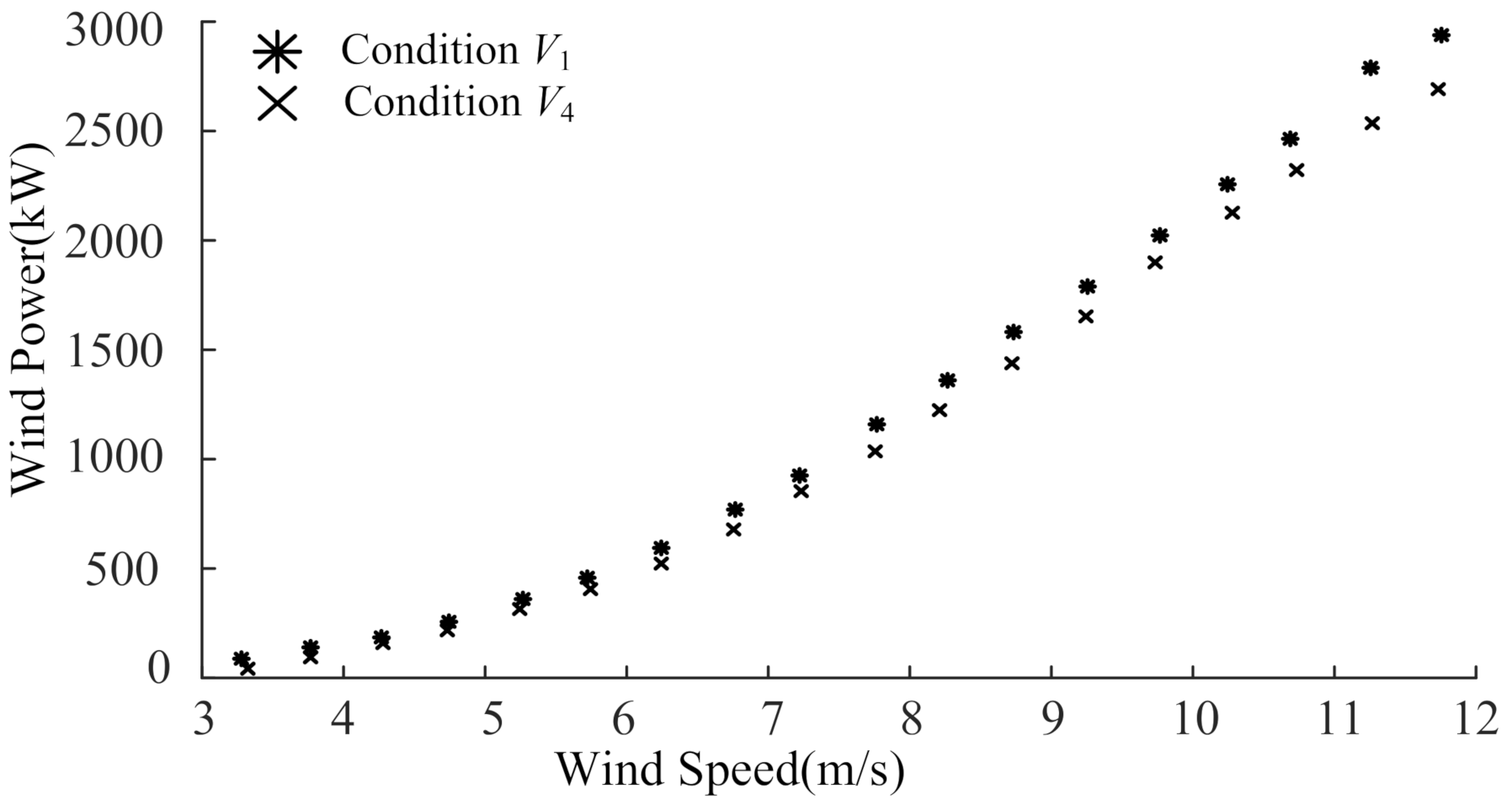
5.1. Variations of Health Conditions to the Power Curves

The OWT has several kinds of operation curve which can be divided into two types. One is the curve between meteorological data and internal variables such as wind speed–power curve, the wind speed–rotor speed curve, and so on. The other is the curve between internal variables such as the rotor speed–power curve, the generator speed–power curve, and so on. The operation curve is an important indicator demonstrating the performance of an OWT. If the health condition of the OWT changes, there will be some deviation from the normal operation curve. Due to the use of internal variables rather than the meteorological data, the curve between internal variables can reflect the abnormality of single component more accurately than the curve between meteorological data and internal variables [41,42,43]. However, it cannot reflect the relationships between the unit condition and wind power. In this paper, the wind speed–power curve is established to show that the output power of wind turbine is not only affected by the external environment, but also affected by the conditions of wind turbine. The random sampling consensus (RANSAC) is introduced to screen the scattered dots painted by the operational data from SCADA; the wind speed is nacelle wind speed. The result is shown as the black dots outline the trend of blue spots in Figure 5.

When the influences of the health conditions of the OWT involved, the operational data will be classified according the defined heal conditions. According to the corresponding wind speed data v_ij and wind power data p_ij screened by RANSAC, a method of bin is introduced to depict the power curved. The power curves with different health conditions are shown in Figure 6.

From Figure 6, it can be found that the deviations between the two power curves with different health conditions are quite obvious which vary with the wind speed. The higher the wind speed is, the bigger the power deviation is. In this case, the power deviation increases from 120 kW under the wind speed of 8 m/s to 250 kW under the wind speed of 12 m/s. The maximal power deviation is about 8% of the rated power. Therefore, the influences of the variations of the OWT conditions is not negligible in offshore WPP.

5.2. CA of the OWT

The scatterplot between the gearbox bearing temperature and the wind speed obtained by RANSAC is shown in the Figure 7. It turns out that the relationship between gearbox bearing temperature and wind speed presents a positive correlation trend. Thus the gearbox bearing temperature is a kind of variable whose values changes with external factors and sometimes the smaller value does not represents a better state. It is very important during FCM evaluation.

Furthermore, an abnormal event in gearbox bearing of wind turbine #24 is selected as an example to demonstrate the process of CA of the OWT. Firstly, according to Figure 4, 21,064 groups (1 year) of historical data of normal operation of the OWT is used to establish the prediction model of gearbox bearing temperature, and another 4320 groups (1 month) of historical data of normal operation is used to verify the accuracy of the model. During the training of LTSM, the main hyper-parameters of the prediction model is set as follows. The number of time steps of input layer is set to be equal to the prediction period (four hours). The number of hidden layer is set to two. The dimension of hidden layer is twice as the dimension of the input data. The validation results (first 1000 groups) of the prediction model are shown in Figure 8.

Then, the prediction value of the gearbox bearing temperature is obtained and illustrated in Figure 8. It can be found that the state around the sampling point 80 is with the lowest temperature. As CA of OWT based on the traditional deterioration degree of the indicator usually takes the rule of the lower the better, the state around the sampling point 80 will be marked as the optimal state. It is a false conclusion for this abnormal event of WT #24.

The dynamic deterioration degrees calculated by (1) and (2) which is also the differences between the predictive value (the blue line) and the actual value (the orange line) in Figure 9 are presented in Figure 10. It can be found that the relative errors of the gearbox bearing temperature prediction are relatively small at the beginning and it begins to fluctuate from the sampling points 60 to 80. Then the prediction error began to increase gradually after sampling the point 100. The prediction error at sampling point 120 is twice as much as the initial one. According to information about the relative errors between the prediction values and the actual values of the indicator, the fluctuation during sampling points 60 to 80 indicates the start point of the given abnormal event. It shows that the proposed CA of OWTs based on the MFCE can detect the abnormal state of the OWT in the early stage and demonstrates a better identifications of OWT failures.

Table 2. Results of MFCE.

Time	Membership Matrix of OWT	Condition of OWT
T1	[1, 0, 0, 0]	V1
T2	[1, 0, 0, 0]	V1
T3	[0.99, 0.01, 0, 0]	V1
T4	[0.88, 0.12, 0,0]	V1
T5	[0.47, 0.53, 0,0]	V2
T6	[0, 0.13, 0.87, 0]	V3
T7	[0, 0, 0, 1]	V4
T8	[0, 0, 0, 1]	V4

shows the membership matrix and the condition of the OWT which are calculated by (16) and (17).

From Table 2 and Figure 10, it can be found that the condition of the OWT kept in the state V₁ from T₁ to T₄ period, while it underwent a minor degradation during T₃–T₄ period which is demonstrated as the membership degree of the condition V₁ gradually decreased from 1 to 0.88 in membership matrix. During T₅–T₆, the deviation between the predicted value and the actual value increased gradually. It represents the deterioration of the gearbox bearings became more serious. The health condition of the OWT turned to V₂ and V₃ in membership matrix. By the period of T₇ and T₈, the temperature of gearbox bearings exceeded the limits, and the condition of the unit was very poor.

The CA of OWTs proposed in this paper can deal with the impact of environmental factors on the evaluation results of the condition of OWT better than the traditional ways, and the results fit the variations of gearbox bearing temperature in Figure 7 very well and demonstrated the variations of the health condition in a more intuitive way. Moreover, it also can show the transformation process of the OWT condition with a high sensitivity through the change of the membership matrix.

5.3. Results of the WPP

In order to verify the effectiveness of the method in this paper, three WPP models is established for comparison. Model I refers to the model presented in this paper. The input of Model I includes the wind speed, the wind direction, temperature, humidity in NWP, and historical wind power, the output of the model is the next four hours of wind power. Model II refers to the direct prediction model that does not consider the conditions of OWTs, while the main parameters are consistent with the Model I. The effects of the health condition of OWT on the WPP are ignored in Model II. Model III refers to the ARIMA model [11] which is one of the most commonly used algorithms for time series of forecasting. The main parameters of Model III is set to (1, 1, 3). The effects of the health condition of OWT to the WPP is also ignored in Model III. The three models are trained with one year operation data (21,064 groups) of OWT. The type of data can be found in Equation (18). A 48 h prediction results (12 prediction periods) are presented here. The comparisons of the three models and the real wind power values are shown in Figure 11.

From Figure 11, it can be found that the results of Model I are more proximate to the practical curve than the other two models. More concretely, in the period before T₅, deviations between the results of Model I and other two models are very small. However, from the time of period T₅ when the health condition of the OWT started to deteriorate, the errors between the WPP result of Model II or Model III and the real data become very considerable. On the contrary, the WPP results of Model I fit the practical data quite well, especially after the time of T₆. With the deterioration going further, the errors between Model II, Model III, and the real data increase gradually while Model I always keeps a good performance. The maximum deviation between Model I, Model II, and Model III can be 600 kW, which is about 20% of the rated power.

Table 3. Prediction error of models.

	Model I	Model II	Model III
RSME (%)	8.74	10.07	10.12
MAE (%)	5.61	7.04	7.13

gives the root-mean-square errors (RSME) and mean absolute errors (MAE) of Model I, Model II, and Model III, respectively. It can be found that Model I has higher accuracy and stability. Compared with Model II and Model III, Model I decreases the RSME 1.38% and MAE1.52%.

6. Conclusions

This paper investigates the impact of health conditions of the OWT on its capability of wind power conversion. An ultra-short time WPP methodology consisting of condition assessment of OWT with MFCE and an OWT condition-based WPP with BP neural network is proposed. The following are the main conclusions:

(1)

Due to the dramatic variation characteristics of the marine environment, variation principles of the monitoring data of an OWT interact with each other as well as the dynamic environment. The proposed MFCE with a new dynamic deterioration of indicators calculated by the relative errors can assess the deterioration of OWTs more accurately and more sensitively.

(2)

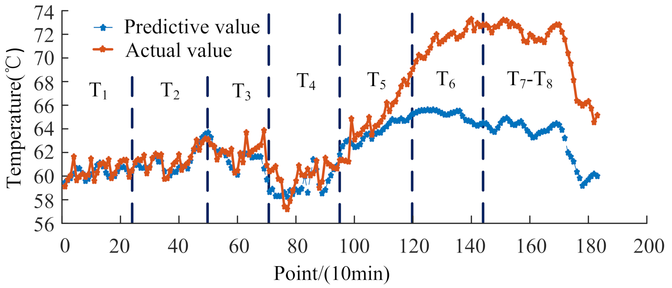
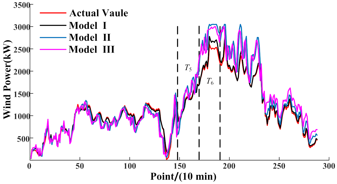
Deterioration of the OWT lowers its output power and will cause a significant error to the result of the offshore WPP. The case study shows that the deterioration condition will lead to a power deviation with about 8% of the rated power.

(3)

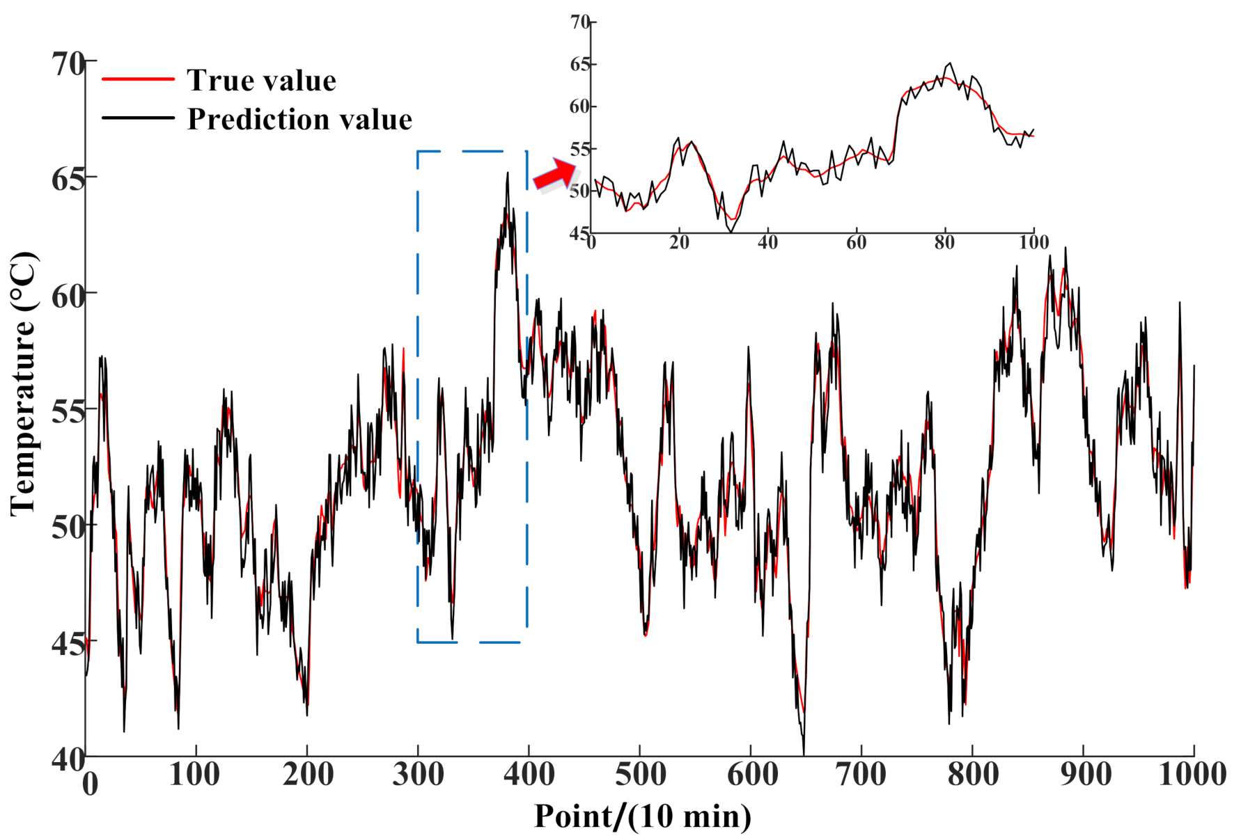
The results of the proposed method and the real power outputs show the effectiveness of the proposed model. Comparing with the traditional direct prediction model without considering the influences of the OWT health conditions, the proposed method improves the accuracy of the prediction result with more than 1% reductions of both RSME and MAE.

(4)

As the variation of the health conditions of the OWTs in the offshore wind farm, the proposed method can be applied to the ultra-short time WPP of the wind farm by aggregating of the individual OWT WPP results.

References

1. Zhao, X.; Cai, Q.; Zhang, S.; Luo, K. The substitution of wind power for coal-fired power to realize China’s CO2 emissions reduction targets in 2020 and 2030. Energy 2017, 120, 164–178. [Google Scholar] [CrossRef]
2. Yang, Y.G.; Liang, G.S. Development of Wind Power Generation and Its Market Prospect. Power Syst. Technol. 2003, 27, 78–79. [Google Scholar] [CrossRef]
3. Zhang, L.; Ye, T.; Xin, Y.; Han, F.; Fan, G. Problems and Measures of Power Grid Accommodating Large Scale Wind Power. Proc. CSEE 2010, 30, 1–9. [Google Scholar] [CrossRef]
4. Peng, X.; Xiong, L.; Wen, J.Y.; Cheng, S.J.; Deng, D.Y.; Feng, S.L.; Wang, B. A Summary of the State of the Art for Short-term and Ultra-short-term Wind Power Prediction of Regions. Proc. CSEE 2016, 36, 6315–6326. [Google Scholar] [CrossRef]
5. Shi, K.P.; Qiao, Y.; Zhao, W.; Huang, S.L.; Liu, Z.J.; Guo, L. Short-term Wind Power Prediction Based on Entropy Association Information Mining of Historical Data. Autom. Electr. Power Syst. 2017, 41, 13–18. [Google Scholar] [CrossRef]
6. Dong, L.; Wang, L.; Khahro, S.F.; Gao, S.; Liao, X. Wind power day-ahead prediction with cluster analysis of NWP. Renew. Sustain. Energy Rev. 2016, 60, 1206–1212. [Google Scholar] [CrossRef]
7. Li, Y.; Wang, Y.; Wu, B. Short-Term Direct Probability Prediction Model of Wind Power Based on Improved Natural Gradient Boosting. Energies 2020, 13, 4629. [Google Scholar] [CrossRef]
8. Zhang, Y.; Sun, H.; Guo, Y. Wind Power Prediction Based on PSO-SVR and Grey Combination Model. IEEE Access 2019, 7, 136254–136267. [Google Scholar] [CrossRef]
9. Fu, Y.; Deng, Z.C.; Shi, S.; Mi, Y.; Liu, D. Offshore Wind Power Forecasting Considering Meteorological Similarity and NWP Correction. Power Syst. Technol. 2019, 43, 1253–1259. [Google Scholar] [CrossRef]
10. Xiong, Y.D.; Liu, K.P.; Qing, L.; Ouyang, T.H.; He, J.Y. Short-term Wind Power Prediction Method Based on Dynamic Wind Power Weather Division of Time Sequence Data. Power Syst. Technol. 2019, 43, 3353–3359. [Google Scholar] [CrossRef]
11. Kavasseri, R.G.; Seetharaman, K. Day-ahead wind speed forecasting using f-ARIMA models. Renew. Energy 2009, 34, 1388–1393. [Google Scholar] [CrossRef]
12. Wang, Y.; Guo, Y. Forecasting method of stock market volatility in time series data based on mixed model of ARIMA and XGBoost. China Commun. 2020, 17, 205–221. [Google Scholar] [CrossRef]
13. Wang, Z.; Lou, Y. Hydrological time series forecast model based on wavelet de-noising and ARIMA-LSTM. In Proceedings of the 2019 IEEE 3rd ITNEC, Chengdu, China, 15–17 March 2019; pp. 1697–1701. [Google Scholar] [CrossRef]
14. Hippert, H.S.; Pedreira, C.E.; Souza, R.C. Combining neural networks and ARIMA models for hourly temperature forecast. In Proceedings of the IEEE-INNS-ENNS IJCNN 2000, Como, Italy, 24–27 July 2000; pp. 414–419. [Google Scholar] [CrossRef]
15. Zhang, C.; Wei, H.; Zhao, J.; Liu, T.; Zhu, T.; Zhang, K. Short-term wind speed forecasting using empirical mode decomposition and feature selection. Renew. Energy 2016, 96, 727–737. [Google Scholar] [CrossRef]
16. De Giorgi, M.G.; Campilongo, S.; Ficarella, A.; Congedo, P.M. Comparison between wind power prediction models based on wavelet decomposition with Least-Squares Support Vector Machine (LS-SVM) and Artificial Neural Network (ANN). Energies 2014, 7, 5251–5272. [Google Scholar] [CrossRef]
17. Yuan, X.; Chen, C.; Yuan, Y.; Huang, Y.; Tan, Q. Short-Term Wind Power Prediction Based on LSSVM–GSA Model. Energy Convers. Manag. 2015, 101, 393–401. [Google Scholar] [CrossRef]
18. Hao, Y.; Tian, C.S. A Novel Two-Stage Forecasting Model Based on Error Factor and Ensemble Method for Multi-Step Wind Power Forecasting. Appl. Energy 2015, 238, 368–483. [Google Scholar] [CrossRef]
19. Zhu, Q.; Li, H.; Wang, Z.; Chen, J.F.; Wang, B. Short-Term Wind Power Forecasting Based on LSTM. Power Syst. Technol. 2017, 41, 3797–3802. [Google Scholar] [CrossRef]
20. Liu, H.; Mi, X.W.; Li, Y.F. Smart deep learning based wind speed prediction model using wavelet packet decomposition, convolutional neural network and convolutional long short term memory network. Energy Convers. Manag. 2018, 166, 120–131. [Google Scholar] [CrossRef]
21. Yin, H.; Ou, Z.H.; Huang, S.Q.; Meng, A.B. A cascaded deep learning wind power prediction approach based on a two-layer of mode decomposition. Energy 2019, 189, 116316–116327. [Google Scholar] [CrossRef]
22. Hu, J.M.; Wang, J.Z.; Ma, K. A Hybrid Technique for Short-Term Wind Speed Prediction. Energy 2015, 81, 563–574. [Google Scholar] [CrossRef]
23. Liu, B.; Zhao, S.; Yu, X.; Zhang, L.; Wang, Q. A Novel Deep Learning Approach for Wind Power Forecasting Based on WD-LSTM Model. Energies 2020, 13, 4964–4981. [Google Scholar] [CrossRef]
24. Niu, Z.; Yu, Z.; Li, B.; Tang, W. Short-term wind power forecasting model based on deep gated recurrent unit neural network. Electr. Power Autom. Equip. 2019, 38, 36–42. [Google Scholar] [CrossRef]
25. Gill, S.; Stephen, B.; Galloway, S. Wind Turbine Condition Assessment through Power Curve Copula Modeling. IEEE Trans. Sustain. Energy 2012, 3, 94–101. [Google Scholar] [CrossRef] [Green Version]
26. Astolfi, D.; Byrne, R.; Castellani, F. Analysis of Wind Turbine Aging through Operation Curves. Energies 2020, 13, 5623. [Google Scholar] [CrossRef]
27. Byrne, R.; Astolfi, D.; Hewitt, N.J. A Study of Wind Turbine Performance Decline with Age through Operation Data Analysis. Energies 2020, 13, 2086. [Google Scholar] [CrossRef] [Green Version]
28. Li, H.; Hu, Y.; Tang, X.; Liu, Z. Method for On-line Operating Conditions Assessment for a Grid-connected Wind Turbine Generator System. Proc. CSEE 2010, 30, 103–109. [Google Scholar] [CrossRef]
29. Xiao, Y.; Wang, K.P.; He, G.J.; Sun, Y.; Yang, X. Fuzzy Comprehensive Evaluation for Operating Condition of Large-scale Wind Turbines Based on Trend Predication. Proc. CSEE 2014, 34, 2132–2139. [Google Scholar] [CrossRef]
30. Huang, B.Q.; He, Y.; Wang, T.Y. Fuzzy Synthetic Evaluation of the Operational Status of Offshore direct-drive Wind Turbines. J. Tsinghua Univ. 2015, 55, 543–549. [Google Scholar] [CrossRef]
31. Yang, M.; Zhou, Y. Ultra-short-term Prediction of Wind Power Considering Wind Farm Status. Proc. CSEE 2019, 39, 1259–1267. [Google Scholar] [CrossRef]
32. Huang, L.; Cao, J.; Zhang, K. Status and Prospects on Operation and Maintenance of Offshore Wind Turbines. Proc. CSEE 2016, 36, 729–738. [Google Scholar] [CrossRef]
33. Zhang, X.M. Performance Analysis and Health Status Evaluation of Wind Turbines Based on SCADA Data. Master’s Thesis, Department of Energy Power and Mechanical Engineering, North China Electric Power University, Baoding, China, 2017. [Google Scholar]
34. Pandit, R.; Kolios, A. SCADA Data-Based Support Vector Machine Wind Turbine Power Curve Uncertainty Estimation and Its Comparative Studies. Appl. Sci. 2020, 10, 8685. [Google Scholar] [CrossRef]
35. Rodríguez-López, M.Á.; Cerdá, E.; Rio, P. Modeling Wind-Turbine Power Curves: Effects of Environmental Temperature on Wind Energy Generation. Energies 2020, 13, 4941. [Google Scholar] [CrossRef]
36. Ciulla, G.; Amico, A.D.; Dio, V.; Brano, V. Modeling and analysis of real-world wind turbine power curves: Assessing deviations from nominal curve by neural networks. Renew. Energy 2019, 140, 477. [Google Scholar] [CrossRef]
37. Wang, Y.; Hu, Q.; Srinivasan, D.; Wang, Z. Wind Power Curve Modeling and Wind Power Forecasting with Inconsistent Data. IEEE Trans. Sustain. Energy 2019, 10, 16–25. [Google Scholar] [CrossRef]
38. Shokrzadeh, S.; Jozani, M.J.; Bibeau, E. Wind Turbine Power Curve Modeling Using Advanced Parametric and Nonparametric Methods. IEEE Trans. Sustain. Energy 2014, 5, 1262–1269. [Google Scholar] [CrossRef]
39. Zhao, H.; Yan, X.; Wang, G.; Yin, X. Fault Diagnosis of Wind Turbine Generator Based on Deep Autoencoder Network and XGBoost. Autom. Electr. Power Syst. 2017, 43, 81–86. [Google Scholar] [CrossRef]
40. Fan, G.F.; Wang, W.S.; Liu, C.; Dai, H.Z. Wind Power Prediction Based on Artificial Neural Network. Proc. CSEE 2008, 28, 118–123. [Google Scholar] [CrossRef]
41. Bi, R.; Zhou, C.K.; Hepburn, D.M. Detection and classification of faults in pitch-regulated wind turbine generators using normal behavior models based on performance curves. Renew. Energy 2017, 105, 674–688. [Google Scholar] [CrossRef] [Green Version]
42. Chen, B.; Matthews, P.C.; Tavner, P.J. Automated on-line fault prognosis for wind turbine pitch systems using supervisory control and data acquisition. IET Renew. Power Gener. 2015, 9, 503–513. [Google Scholar] [CrossRef] [Green Version]
43. Sun, Q.L.; Liu, C.L.; Zhou, Y. Abnormal detection of operation conditions of wind turbine based on state curve. Therm. Power Gener. 2019, 48, 110–116. [Google Scholar] [CrossRef]
Figure 1. Framework of offshore WPP.
Energies 14 00891 g001
Figure 2. Process of CA of the OWT.
Energies 14 00891 g002
Figure 3. Evaluation system of OWTs.
Energies 14 00891 g003
Figure 4. Structure of LSTM.
Energies 14 00891 g004
Figure 5. Result of RANSAC for the operational data.
Energies 14 00891 g005
Figure 6. Power curves in different conditions.
Energies 14 00891 g006
Figure 7. Scatterplot between gearbox bearing temperature and wind speed.
Energies 14 00891 g007
Figure 8. Validation results of the prediction model.
Energies 14 00891 g008
Figure 9. Actual and prediction value of gearbox bearing temperature.
Energies 14 00891 g009
Figure 10. Relative error of Gearbox bearing temperature.
Energies 14 00891 g010
Figure 11. Results of wind power prediction.
Energies 14 00891 g011