What Is the Effect of Outer Jacket Degradation on the Communication Parameters? A Case Study of the Twisted Pair Cable Applied in the Railway Industry

Abstract

Among the variety of problems encountered in transmission lines, the outer jacket degradation-derived faults of communication cables in railway applications have a significant impact on the transmission line parameters, especially if the cables are exposed to extremely varying environmental conditions, such as temperature deviation and humidity changes. In this paper, an advanced model of a twisted pair communication cable is proposed, together with approximated degradation functions for distributed parameters of the model, such as the shielding inductance, resistance, and capacitance per meter of cable length. This allows for gathering the distributed parameters for the proposed model under specific environmental conditions. The degradation functions for the parameters have been identified and compared with simulation results, including the communication speed and frequency band, and it has been confirmed that the transmission reliability depends on the cable condition. The authors discuss the influence of outer jacket degradation on signal behavior in terms of time and frequency domains that should be considered while developing new signaling devices for railway transportation.

1. Introduction

Safe and reliable railway systems contribute to the higher speed of trains and capacity of track sections, thereby enabling railways to develop and increasing their importance as a cost-effective and efficient mode of transport [1]. Cable connections are among the most important parts of a distributed rail traffic control system [2]. However, one of the major issues is the lack of validated models for special communication cables that are used in railways. There is also no research on outer jacket faults and on how such faults change distributed parameters of the communication cable. They are usually exposed to outdoor environmental conditions such as temperature, solar radiation, water, or mechanical damage [3,4,5]. A common approach to signaling is to use a four-wire cable containing a power supply pair and communication pair of wires. The railway systems occupy a large area [6] and communication cables may be thousands of meters long (sometimes up to 15 km). For safety reasons, the outer shield (outer jacket) of such cables is made of a special type of polyvinyl chloride with an increased resistance to external factors (aggressive), which results in its reduced elasticity (i.e., a reduced content of plasticizers). Over a long period of time, the reduced elasticity leads to outer jacket degradation (porosity and roughness). Then, due to the weather and temperature, water freezes and results in further outer jacket degradation. The observed situation may lead to unpredictable railway system behavior that is very important from a maintenance point of view. In general, there is a lack of information that would take into account a “soft” fault of an outer jacket in transmission cables. Sometimes, as is described in [7], the system wiring is tested, but it happens extremely rarely and is expensive. Therefore, current and near future maintenance methods and preventive maintenance algorithms expect understanding of the current status of the used components.

The so-called “soft” fault may be the result of outer jacket damage or an aging effect—parameters of electronic components, connections, and transmission lines are subject to an aging effect. Selected aspects of accelerated aging of the insulation of power cables (the impact of temperature and radiation) are described in [8,9]. Unfortunately, the up-to-date literature provides no solution (lack of a model) for the impact of a specific fault condition (caused by the outer jacket) on the transmission reliability (lost communication) within railway communication. For communication networks in general, the physical phenomena that occur inside cables during operation, and their influence on the remaining lifetime, are not fully understood [8]. The quality of the transmitted information depends on the condition of the wires, so it is important to know how the time and frequency domains of the distributed parameters behave. Most research has paid attention to the diagnosis of catastrophic faults (open and short circuits [10]) in cables, but there has been much less research on parametric faults, which cause a small change [11] in the impedance characteristic [12]; however, this very commonly appears in a real environment [13]. Various field test methods are listed in [14]. The problem of fault diagnosis, especially in electronic analog and mixed-signal devices [15,16], is an important challenge in terms of predictive maintenance [17]. The modeling of transmission lines is another issue which, on the one hand, is important, but on the other hand, is very challenging due to, e.g., aging effects [18], outer jacket damage, and shunt parameters. From a practical point of view, a correct model is essential for the simulation and further validation of equipment under specific test scenarios.

The main objective of this work is to propose a single segment model with its distributed parameters for three types of cable and then perform a simulation of the transmission cables. Moreover, specific railway safety rules require the grounding of one end of the circuit and galvanically isolating the remote device(s). Due to environmental conditions (high voltage and currents [19,20]), there is a need to create robust devices and galvanic isolation is used to increase the input impedance to disturbances. Without such features, the wheel detectors will not have a significant advantage over track circuits. Such a connection diagram of a railway installation is shown in Figure 1.

A specific benefit is expected from such a model description. It allows for software analysis and may provide information about signal parameters and cable conditions (i.e., if it is about to be damaged to give enough time to call the service support team). This model is also a very desirable solution in a problematic situation when the access to a test object is restricted by law and must be operated under the supervision of authorized personnel or even under a military guard. The proposed diagram may also be helpful when there are time constraints for shutting down at least part of the traffic management system. The introduced diagram may have a significant impact on the capacity and availability of railway lines and may result in a reduced maintenance intervention time for the rail operator.

2. Proposed Model of an Elementary Part of a Transmission Line

There are several approaches to modeling transmission lines described in the literature. Most of them are based on a single segment of the transmission line and comprise parameters that are based on the unit of length, including the resistance, inductance, capacitance, and conductance. The models describe a single pair of the communication line (usually twisted) that is shielded. However, these papers do not describe the real environmental conditions in railway applications due to the use of simplified models and incorrect connections of elements.

In [21], the authors only focused on the radiation immunity of single twisted pairs in an ideal situation with conducting ground. In [22], an equivalent circuit representation is developed with merely a single unshielded pair of wires. In [23], a simulation with no shielding and grounded load is presented, which is untypical in railway applications. This model could be used in three-phase power distribution systems, in long-distance applications.

However, both of the above configurations are non-compliant with the presented concept of cabling used in railway applications, where shielded with unshielded twisted pairs are usually employed.

Other kinds of problems may be noticed, e.g., connecting shield at both ends of the cable [24,25], which is contrary to generally accepted principles for noncoaxial cables, because no current can flow through it in a standard configuration. The grounding of a long-distance device presented in [17] is also not compliant with the requirements for railway applications, where the wayside equipment is usually galvanically isolated from the communication and power line.

Communication cables in the railway industry do not need to fulfill special safety requirements, because the safety mechanism is implemented in the communication protocol to prevent an unpredictable situation. Therefore, there is no common earth at the input and output. This is a justifiable reason to create a much more realistic and typical railway industry scheme for signaling cables, which may also be used during an analysis of the impact of outer jacket faults on transmission lines. Therefore, the authors claim that a model description is not sufficient and does not reflect the real conditions that can be observed in the railway industry.

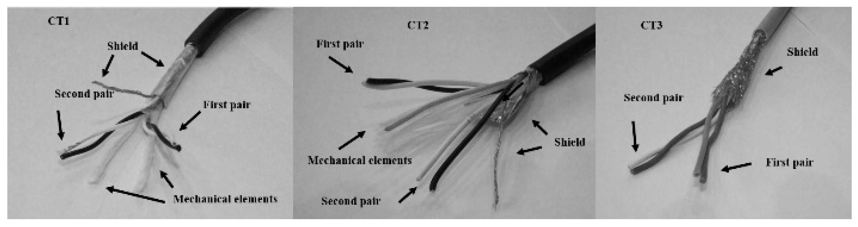
3. Cable Construction

The assumed definition of a communication model is an aspect of major importance. The distributed parameters of the transmission line can be introduced, but the twisted pair communication cables applied in the railway industry require an individual approach.

A simplified view of a typical cable used to connect wayside equipment is presented in Figure 2.

The cable consists of the following:

• Two pairs of twisted wires: The first for the power supply and the second for digital communication;
• An electrical shield increasing the immunity against external disturbance;
• Mechanical elements to increase the mechanical resistance (e.g., protect against burst);
• An outer jacket protecting internal parts of cables against environmental conditions.

Various types of cables are used in railway applications. Sometimes, it is necessary to use a cable with unknown parameters, which has been used on site to-date, but in a new application for long distances of up to 15 km, the use of a type 2 cable (identified as ‘CT2’) is recommended. For middle distances, a type 1 cable (identified as ‘CT1’), but sometimes also a type 3 cable, is applied (identified as ‘CT3’) with a relatively short distance. These are the most commonly used cable types in a railway application. All aforementioned cables are shown in Figure 3.

The basic distributed parameters provided by the manufacturer are shown in

Table 1. Distributed parameters of CT1, CT2, and CT3.

Cable Parameters	Type 1 Cable (CT1) RE-2Y(ST)Y 2 × 2 × 0.75 mm2	Type 2 Cable (CT2) RE-2Y(ST)Y 2 × 2 × 1.3 mm2	Type 3 Cable (CT3) -CY 2 × 2 × 1.0 mm2
Loop resistance (Ω/km)	52	28.4	-
Mutual capacitance (nF/km)	60	75	0.135
Inductance (mH/km)	0.7	0.7	-
Insulation resistance (GΩ/km)	5	5	0.1

.

The main objective is to develop a model of the transmission line with degradation parameters resulting from a soft fault of an outer jacket. A prominent problem arises when only one end of the circuit is grounded and the remote device(s) is(are) isolated galvanically. Such a connection diagram of a railway installation is shown in Figure 1.

Therefore, the authors introduce an innovative elementary single segment of a railway cable, which is presented in Figure 4. Each pair of a cable has input and output points, described as In1A/Out1A and In1B/Out1B in the first pair, and In2A/Out2A and In2B/Out2B in the second pair. ShieldIn/ShieldOut are the input/output of the shield. The capacitance between each line and shield to ground capacitance are among the major factors which have a huge influence on the quality of signaling. Moreover, the working conditions change the cable parameters at the input/output (installation points) under humidity and temperature (environmental conditions). The same influence can be observed with respect to the soft fault of an outer jacket at any point along the cable.

An innovative model of a shielded twisted pair cable is proposed below, for use in railway applications for signal analysis. Among a variety of parameters, it also has multiple capacitance between the wires and different types of shield connections that are used in railway applications.

A detailed description of the elements presented in Figure 4 is as follows:

R_W—wire resistance; L_W—wire inductance; C₁₁, C₁₂—capacitance between the wires in the same pair; C₇, C₈, C₉, C₁₀—capacitance between different wires; C₂, C₃, C₄, C₅—capacitance between a wire and shield; C₆—capacitance between the shield and ground; R₃, R₄, R₅, R₆—resistance between a wire and shield; R_S—resistance of the shield; and L_S—inductance of the shield.

4. Setup of a Soft Fault of the Outer Jacket

There are papers available [26,27,28,29] that discuss cable parameter degradation over a specific time period, but they are only focused on the isolation parameters for a high and medium voltage. However, distributed parameters change over time, and the most important change is derived from outer jacket faults because they are usually soft and do not generate a transmission fault. It is very difficult to describe precisely when the soft fault of an outer jacket occurs, but the influence on the transmission between input and output devices may affect the normal operation. Railway signaling has historically been based on current loops and relays, but due to cost-savings and the increasing number of wayside equipment in use, digital transmission is implemented. The Controller Area Network (CAN) differential serial communication system is one of the most frequently used for signaling systems, because of its flexibility and immunity to external electromagnetic influences. High speed CAN transmission (e.g., 500 kb/s) is used for short distance devices to transmit a lot of data and low speed CAN transmission (e.g., 10 kb/s) is used for field devices which exchange small packages of data, but even this limitation of the baud rate parameters of cables has a huge impact on the system availability. This is due to the length of the whole transmission line, which may be up to 4 km long. An overview of the general problem is shown in Figure 5. The following are presented: The source of disturbances; an equivalent diagram of cables; and interfaces of long-distance devices.

In the case of industrial procedures, the immunity testing of objects is performed by exposing them to extreme environmental conditions for a defined period of time [30]. In this study, the influence of water was selected, because it significantly influences the parameters of signaling cables in railway applications. This is the worst case scenario because the cable is usually buried under the ground and it can be surrounded by water and exposed to mechanical damage.

Three types of 10 m long cables were placed in a vessel with water (together with both ends of the cables). The water level was set to 30 cm high and salinity was set to 2.5% of weight. The cable length was required for measuring the instrument accuracy and physical restrictions. Samples were kept under water for four weeks. Based on the changes of parameters, the next period of measurement was defined. The scheme of the experiment is shown in Figure 6.

All of the measurements were performed by a Wayne Kerr 6500 unit (a specialized multivariable measurement tool [31]) with clamps no. 1EVA40100:

• R_W—resistance of the wire: Measured between both ends of the wire, with the other terminals open;
• Lw—inductance of the wire: Measured between both ends of the wire, with the other terminals open;
• R_S—resistance of the shield: Measured between both ends of the shield, with the other terminals open;
• L_S—Inductance of the shield: Measured between both ends of the shield, with the other terminals open;
• C₁₁—capacitance measured between wires in the first pair at one end, with the other terminals open;
• C₁₂—capacitance measured between wires in the second pair on one end, with the other terminals open;
• C₂₃ = C₂ + C₃, (C₂ = C₃)—capacitance measured between the first pair and shield at one end, with the other terminals open;
• C₄₅ = C₄ + C₅, (C₄ = C₅)—capacitance measured between the second pair and shield at one end, with the other terminals open;
• C₇₁₀ = C₇ + C₈ + C₉ + C₁₀, (C₇ = C₈ = C₉ = C₁₀)—capacitance measured between the first and the second pair (short wires in pairs) at one end, with the other terminals open.

Some measurements, like those of the capacitance and inductance, were conducted for the three frequencies of 1, 10, and 100 kHz. See below for the selected results (

Table 2. Measurement results of CT1 (n = 0 stands for the nominal parameters of the cable).

Days in Salt Water (n)	RW, mΩ (20 Hz)	Lw, µH (10 kHz)	RS, mΩ (20 Hz)	LS, µH (20 Hz)	C11, pF (10 kHz)	C12, pF (10 kHz)	C23, nF (10 kHz)	C45, nF (10 kHz)	C710, nF (10 kHz)
0	364.25	14.5	280	10.2	490	475	1.50	1.49	0.80
1	375.75	14.4	300	11.1	530	510	1.58	1.53	0.86
2	374.50	14.6	290	10.5	550	520	1.60	1.54	0.86
5	375.75	14.7	320	10.8	610	590	1.80	1.75	0.89
7	375.75	14.5	320	11.0	610	600	1.92	1.85	0.89
14	382.00	14.8	325	11.2	660	650	2.10	2.20	1.20
21	379.25	14.5	330	11.0	700	700	2.50	2.40	1.40
28	379.50	14.6	331	10.9	720	700	2.70	2.60	1.40
${\mathsf{\delta }}_1$ (%)	4.2	0.7	18.2	6.9	46.9	47.4	80.0	74.5	75.0
${\mathsf{\sigma }}_1$ (-)	4.99	0.12	18.15	0.31	76.72	80.89	0.41	0.40	0.24

for CT1,

Table 3. Measurement results of CT2 (n = 0 stands for the nominal parameters of the cable).

Days in Salt Water (n)	RW, mΩ (20 Hz)	Lw, µH (10 kHz)	RS, mΩ (20 Hz)	LS, µH (20 Hz)	C11, pF (10 kHz)	C12, pF (10 kHz)	C23, nF (10 kHz)	C45, nF (10 kHz)	C710, nF (10 kHz)
0	133.50	11.5	270	10.0	560	540	1.10	1.10	1.00
1	134.25	11.5	270	10.0	880	840	3.70	3.70	1.00
2	133.25	11.6	275	11.0	1000	970	4.28	4.07	2.02
5	133.75	11.3	320	12.0	1080	985	4.40	4.35	2.04
7	133.50	11.4	320	11.0	1100	995	4.50	4.40	2.05
14	132.25	11.6	350	12.0	1120	1120	5.00	4.55	2.30
21	131.00	11.5	360	13.0	1140	1100	5.10	4.63	2.50
28	131.75	11.6	365	10.0	1160	1120	5.20	4.78	2.60
${\mathsf{\delta }}_2$ (%)	−1.3	0.9	35.2	0.0	107.1	107.4	372.7	334.5	160.0
${\mathsf{\sigma }}_2$ (-)	1.05	0.10	37.81	1.05	188.35	181.50	1.25	1.12	0.58

for CT2, and

Table 4. Measurement results of CT3 (n = 0 stands for the nominal parameters of the cable).

Days in Salt Water (n)	RW, mΩ (20 Hz)	Lw, µH (10 kHz)	RS, mΩ (20 Hz)	LS, µH (20 Hz)	C11, pF (10 kHz)	C12, pF (10 kHz)	C23, nF (10 kHz)	C45, nF (10 kHz)	C710, nF (10 kHz)
0	250.75	9.6	100	12.0	1050	1020	2.60	2.46	1.51
1	252.00	11,3	104	10.5	1140	1120	3.13	3.26	1.85
2	250.75	9.8	101	10.3	1210	1190	3.65	3.50	2.04
5	250.50	10.0	106	12.0	1500	1550	4.70	4.60	2.60
7	250.75	10.8	108	11.0	1640	1750	5.60	5.40	2.90
14	245.00	10.1	110	12.0	1920	2020	7.60	7.30	4.00
21	245.00	10.0	112	11.0	2050	2050	8.10	8.00	4.00
28	248.75	10.2	111	13.0	2100	2100	8.30	8.20	4.10
${\mathsf{\delta }}_{3 }(\%)$	−0.8%	6.3%	11.0%	8.3%	100.0%	105.9%	219.2%	233.3%	171.5%
${\mathsf{\sigma }}_3 (-$)	2.73	0.56	4.16	0.68	361.48	396.97	2.00	1.94	0.93

for CT3) of 10 m long cables for the model shown in Figure 4. To compare changes in parameter values, the following statistical parameters were used:

• Relative error:

$$\mathsf{\delta }=\frac{x-x_0}{x_0}\ast 100\%,$$

(1)

where $x_0$—parameter value before the degradation experiment, and $x$—parameter value after 28 days of degradation.

• Standard deviation:

$$\mathsf{\sigma }=\sqrt{\frac{{{\displaystyle \sum }}_{i=1}^n(x_i-{\overline{x)}}^2 }{n-1}},$$

(2)

where $x_i$—sample value, and $\overline{x}$—arithmetic average of samples.

It was quite surprising that the changes (${\mathsf{\delta }}_1$) in the capacitive parameters (Table 2) were the most significant (C₁₁ increased by 46.9%, C₁₂ increased by 47.4%, C₂₃ increased by 80.0%, C₄₅ increased by 74.5%, and C₇₁₀ increased by 75.0%). This was due to water penetrating the empty space in the structure of the cable and changing the dielectric permittivity. Parameters R_W, L_W, and L_S were not affected by salt water. An increase of 18.2% of the parameter R_S was caused by its mechanical structure, because it is made of an aluminum shield and steel wire, which can be damaged by salt water. The conclusions are confirmed by the standard deviation (${\mathsf{\sigma }}_1$), which is used to minimize measurement errors.

Based on the results (Table 3) of CT2 measurements, the biggest changes (${\mathsf{\delta }}_2)$ to capacitive parameters could also be observed (C₁₁ increased by 107.1%, C₁₂ increased by 107.4%, C₂₃ increased by 372.7%, C₄₅ increased by 334.5%, and C₇₁₀ increased by 160%). The shield had a similar mechanical structure to the CT1 cable, so a decrease of the shield’s factor could be observed (R_S increased by 35.2%). In this case, the standard deviation (${\mathsf{\sigma }}_2)$ value also confirmed the deviation of parameters.

In the case of the CT3 (Table 4) measurement, the capacitive parameter change (${\mathsf{\delta }}_3)$ was also significant (C₁₁ increased be 100.0%, C₁₂ increased by 105.9%, C₂₃ increased by 219.2%, C₄₅ increased by 233.3%, and C₇₁₀ increased by 171.5%), similar to the previous types of cables. However, due to a different kind of shield design, the shield parameters did not change so much (R_S increased by only 11%) compared to CT1 and CT2. Likewise, the value of the standard deviation (${\mathsf{\sigma }}_3)$ corresponds to the deviation parameters.

5. Approximation of Parameters for a Segment

Faults in transmission can be investigated on a hardware and software level. Usually, conductivity is measured on the hardware level and a much more complex diagnosis can be made on the software level. In order to create a diagnostic test for the assumed environmental conditions, the outer jacket degradation due to a soft fault must be analyzed. In previous sections, a twisted pair cable model was proposed, and the degradation of parameters was measured for various cable types used in railway applications. The goal of this section is to provide a reliable approximation function for the degradation of elements of segments of a long transmission line. Due to the nature of the phenomena and acquired data that are shown in Table 2, Table 3 and Table 4, the authors chose the following functions:

• Logarithmic:

$$f_1\left(t\right)=a·log\left(t+1\right)+b,$$

(3)

• Polynomial 2 order:

$$f_2\left(t\right)=a{t}^2+bt+c,$$

(4)

• Exponential type 3:

$$f_3\left(t\right)=a+b\left(1-e^{-t/\mathsf{\tau }}\right),$$

(5)

where $t-days in water.$

Cable parameters were split into two groups. The first one contained parameters with insignificant change (deviation value below 40%), such as R_W, L_W, R_S, and L_S. This one will be omitted in the rest of the analysis. The second one, consisting of cable parameters with significant change (deviation value above 40%), included C₁₁, C₁₂, C₂₃, C₄₅, and C₇₁₀. The quality of approximations was evaluated based on the R² parameter, which is a coefficient of determination—a statistical measure of how well the regression predictions approximate the real data points. MATLAB environment and collected measurement results were used for the purpose of approximation function calculations. Values of R² for selected cable parameters are presented in

Table 5. R² parameter of function approximation for CT1, CT2, and CT3.

Approxi-mation Function	R2 for C11			R2 for C12			R2 for C23			R2 for C45			R2 for C710
	CT1	CT2	CT3	CT1	CT2	CT3	CT1	CT2	CT3	CT1	CT2	CT3	CT1	CT2	CT3
$f_1\left(t\right)$	0.989	0.786	0.973	0.981	0.822	0.964	0.884	0.747	0.962	0.899	0.666	0.961	0.795	0.870	0.956
$f_2\left(t\right)$	0.967	0.671	0.994	0.982	0.723	0.979	0.991	0.625	0.997	0.997	0.539	0.997	0.948	0.796	0.989
$f_3\left(t\right)$	0.983	0.988	0.998	0.990	0.936	0.991	0.991	0.956	0.994	0.997	0.981	0.994	0.946	0.863	0.984

.

A better approximation quality means that R²→1, so based on the result presented in Table 5, the best approximation of the degradation parameters gives function $f_3\left(t\right).$ As expected, it has a limitation in +∞, because the capacitive parameters must be limited in a long period of time, due to its finite empty space in the cable, which can be penetrated by water:

$$\underset{t\to \infty }{\lim }f\left(t\right)=\underset{t\to \infty }{\lim }\left(a+b\left(1-e^{-t/\mathsf{\tau }}\right)\right)=a+b, \mathsf{\tau }>0.$$

(6)

R² in respect of function $f_2\left(t\right)$ is also good but is not monotonic and it does not have a limited value when t→+∞. Similar conclusions are applicable to $f_1\left(t\right),$ as it also does not have a limitation in +∞. In summary, $f_1\left(t\right)$ and $f_2\left(t\right)$ were rejected due to the aforementioned disadvantages. Therefore, the exponential formula was selected to describe the degradation parameters. Detailed $f_3\left(t\right)$ parameters calculated in the MATLAB environment are shown in

Table 6. Formula of degradation function approximations using function $f_3\left(t\right)$.

Parameters	CT1	CT2	CT3
C11 [pF@10 kHz]	a = 502.2	a = 564.3	a = 1026
	b = 221.9	b = 559.2	b = 1139
	τ11 = 9.416	τ21 = 1.287	τ31 = 9.320
C12 [pF@10 kHz]	a = 479.6	a = 545.7	a = 971.5
	b = 233.7	b = 524.3	b = 1161
	τ12 = 9.183	τ22 = 1.288	τ32 = 6.993
C23 [nF@10 kHz]	a = 1.771	a = 1.121	a = 2.534
	b = 0.01537	b = 3.716	b = 6.360
	τ13 = 59.347	τ23 = 0.916	τ33 = 10.207
C45 [nF@10 kHz]	a = 1.460	a = 1.114	a = 2.514
	b = 1.821	b = 3.41	b = 6.345
	τ14 = 28.377	τ24 = 0.766	τ34 = 11.210
C710 [nF@10 kHz]	a = 0.7868	a = 0.9977	a = 1.495
	b = 1.663	b = 1.476	b = 2.818
	τ15 = 54.705	τ25 = 4.286	τ35 = 9.001

.

According to Table 6, the following can be said: “a”—parameter defines the capacitance before the degradation test (CN); “b”—parameter defines the change in capacitance during the degradation test (ΔC); “a + b” = (CN + ΔC)—define the expected final value after the degradation process; and “τ”—parameter defines the number of days when the capacitance increased by 63.2%. The physics of the phenomenon suggests that the change of the τ parameters will be proportional to the length of the cable. The tested cables are 10 (m) long, and if their length is increased to 100 (m), then the τ value will increase 10 times in the same conditions of a testing environment. A different value of τ for each type of parameter (τ_1n ≠ τ_2n ≠ τ_3n, n = 1, 2, 3) could have been caused by a different mechanical structure of CT1, CT2, and CT3 cables. Moreover, the manufacturing date of each cable was unknown and they had been stored in various conditions, which could have resulted in different initial conditions, but this was very difficult to avoid, because, even during transport, the cable could have contact with water, especially when transported by sea.

An anomaly in the results of the measurement can be observed with respect to τ₁₃ or τ₁₄, because, based on this type of parameter (C₂₃ and C₄₅) for other cables (τ₂₃ ≈ τ₂₄, τ₃₃ ≈ τ₃₄), they should have similar values. Analogous observations were made for C₁₁ and C₁₂ (τ₁₁ ≈ τ₁₂, τ₂₁ ≈ τ₂₂, τ₃₁ ≈ τ₃₂). This could have been caused by measurement difficulties (oxides formed at the ends of the wires), which create additional impedance between the tested object and probes.

The design parameters of the cable have a huge impact on the model parameters, which is particularly visible between the CT2 cable and the CT1 and CT3 cables (capacitance C₁₁ and C₁₂ are about two times higher, respectively, and the shield resistance is about three times lower—Table 6). This design also has an extensive influence on the speed of filling the empty spaces in the cable with water, which, due to its electrical permeability, which is much higher than air, results in an increase in all parasitic capacitance values. The design of the shield and the diameter of signal cables and external insulation are very important. In the case of a CT1 cable, the shield in the form of a metal foil and a plastic foil wraps the signal cables quite tightly, which results in a fairly high value for the time constant (τ₁₃, τ₁₄, and τ₁₅) corresponding to a long time of filling the empty spaces in the cable with water. At the same time, due to capillary phenomena occurring in twisted signal cables, lower values of time constants τ₁₁ and τ₁₂, compared to τ₃₁ and τ₃₂, of the CT3 cable were observed. In the case of the CT3 cable, the shield consists of a metal braid only, without any additional plastic film. This results in a faster filling of the empty spaces in the cable with water (lower values of τ₃₃, τ₃₄, and τ₃₅, compared to τ₃₁ and τ₃₂). Water penetrates the CT2 cable the most quickly, which probably results from its largest diameter. This cable also has the largest diameter among signal cables, and thus has the largest voids inside the transmission line.

Filling of the empty spaces in a cable does not significantly affect its inductance L_S because water is a diamagnetic. The salt water environment practically does not affect the resistance of copper signal wires, which also have tight insulation.

Examples of the approximation of C₁₂ and C₂₃ by function $f_3\left(t\right)$ are shown in Figure 7. Function $f_3\left(t\right)$ estimates the measured parameters and enables them to be predicted in the future—the actual moment of degradation can be estimated with the use of the proposed function.

6. Impact of Soft Fault-Derived Parameter Degradation on a Transmission Line

The most important part from an application point of view is to use the selected approximation function ($f_3\left(t\right)$) to signal parameter simulation, i.e., bandwidth and group delay. The signal parameters were determined in the time slots 0, 5, 15, 25, and 50 T. 0 T defines the cable parameters before degradation, 5 T describes the parameters of cables after 5 days of artificial degradation, and 15 T is equivalent to 15 days of accelerated artificial degradation, etc.

The entire simulation was performed using LTSpice. It was assumed for the purpose of examining the transmission line parameters that a long-distance cable would contain 10 m of elementary parts (a relevant scheme is proposed in Figure 4). An overview of the simulation is shown in Figure 8.

Module 1 consists of a source of the signal ($V_{IN})$ and line termination, i.e., a resistor of 120 Ω. In Module 2, N = 250 elementary parts of a transmission line (shown in Figure 4) simulate 2.5 km of a wayside cable. The configuration is an approximation of real-life conditions, when a group of wheel detectors are located ca. 2.5 km from the relay room where the master CAN bus is installed, so 1.5 km of cable is available for connecting devices in the group of wheel detectors. Therefore, the total length of the CAN transmission line is limited to 4 km. Module 3 consists of line termination: A resistor of 120 Ω ($V_{OUT})$.

To define the parameters, we evaluated the following:

• Amplitude characteristics on a logarithmic scale:

$$K_L\left(\omega \right)=20log\frac{V_{OUT}\left(\omega \right)}{V_{IN}\left(\omega \right)} [\mathrm{dB}],$$

(7)

where $V_{OUT}(\omega$)—output voltage in the frequency domain, and $V_{IN}(\omega$)—input voltage.

• Group delay:

$${\tau }_{\varphi }=-\frac{d\varphi }{d\omega },$$

(8)

where ϕ(ω)—phase shift.

Simulations were performed for 0, 5, and 50 T marked in green, blue, and red, respectively, to evaluate the outer jacket degradation on the basis of a model proposed. The amplitude and group delay characteristics of the three types of cables are presented below. For the CT1 type of cable (Figure 9), the degradation process is smooth, and there are no rapid changes like in the case of CT3.

Negative peaks (and rapid changes) of the group delay characteristics are caused by the numerical limitation of the LTSpice environment, and when the phases exceed the range of the [−π, +π], it is usually normalized. For CT2, the lowest value of voltage dumping for 1 kHz could be observed (see Figure 10), which is consistent with the physical parameters (lowest resistance in Table 1). In this case, the degradation process is rapid.

In the case of CT3 (Figure 11), the largest change in the voltage damping value can be observed at a 1 kHz frequency and the degradation process is also smooth.

The characteristic parameters for all cables with respect to degradation are presented in

Table 7. Impact of degradation on the communication parameters of cables (constant length l = 2.5 km).

Type of Cable	CT1
Time slot, T	0	5	15	25	50	${\mathsf{\delta }}_{CT1}$
Cut-off frequency −3 dB (kHz)	14.26	12.85	11.58	10.44	9.40	−34.08%
Group delay, µs (1 kHz)	39.25	43.68	49.15	53.46	58.56	+49.20%
$f_{Zin}^P$ (kHz)	1283	1191	1077	956.75	1027	−19.95%
$Z_{IN}^P$$(f_{Zin}^P)$ (kΩ)	1.406	1.140	0.9290	1.239	0.9082	−35.40%
Type of Cable	CT2
Time slot, T	0	5	15	25	50	${\mathsf{\delta }}_{CT2}$
Cut-off frequency −3 dB (kHz)	17.4	8.51	8.45	8.42	8.39	−51.78%
Group delay, µs (1 kHz)	29.15	51.31	52.50	52.60	52.61	+80.48%
$f_{Zin}^P$ (kHz)	1378	916.50	878.56	877.34	877.34	−36.36%
$Z_{IN}^P$$(f_{Zin}^P)$ (kΩ)	2.321	1.229	1.223	1.129	1.129	−51.36%
Type of Cable	CT3
Time slot, T	0	5	15	25	50	${\mathsf{\delta }}_{CT3}$
Cut-off frequency −3 dB (kHz)	10.33	6.96	5.38	4.95	4.79	−53.63%
Group delay, µs (1 kHz)	47.29	74.62	96.34	102.04	104.34	+120.64%
$f_{Zin}^P$ (kHz)	1177	873.60	744.95	712.13	700.86	−40.45%
$Z_{IN}^P$$(f_{Zin}^P)$ (kΩ)	1.970	1.424	1.029	930.93	872.53	−55.71%

. To evaluate the change of the measured parameters, a relative error was introduced:

$${\mathsf{\delta }}_{CT}=\frac{x_T-x_0}{x_0}\ast 100\%,$$

(9)

where $x_0$—parameter value before degradation, and $x_T$—approximated parameter value after 50 T of the degradation process.

Based on the performed simulations for 2.5 km long cables that are shown in Table 7 (approximated by 250 elementary parts of a transmission line—shown in Figure 7), it was concluded that the highest change in cut-off frequency (−3 dB) after 50 T could be observed for CT3 (decreased by 53.63%), and a similar result was noticed for CT2 (decreased by 51.78%) and CT1 (decreased by 34.08%). The cut-off frequency is similar to the 10 kb/s carrier frequency of communication signals (10 kHz), and due to the non-monotonic shape of frequency characteristic and CAN sampling algorithm, it is very difficult to define the frequency which caused the transmissions errors.

However, a much more interesting conclusion can be drawn from the measurement results of the group delay caused by the degradation of an outer jacket. It was proved that after a sufficiently long period of time, the fault under analysis made transmission impossible because the delay time exceeded the maximum allowed value specified by CAN transmission (the results concern cables that are 2.5 km long). Even if the device is designed with a required margin of delay, e.g., 20%, the degradation makes cable CT1 unusable after 25 T (time slots), cable CT2 unusable after 5 T (time slots), and cable CT3 unusable after approximately 1 T (time slot). It is expected that shorter lines are more robust and the problem should disappear for cables shorter than 2.5 km for CT1 and CT2, and more than 1.5 km for CT3. Values can be estimated based on the steady state condition of parameters and designed approximation functions.

The next simulation is linked to the variation of the input impedance parameters of the transmission line because of outer jacket degradation:

$$Z_{IN}\left(\omega \right)=\frac{V_{IN}\left(\omega \right)}{I_{IN}\left(\omega \right)},$$

(10)

where $V_{IN}(\omega$)—voltage at the input of the transmission line, and $I_{IN}(\omega$)—current in the input of the transmission line.

$Z_{IN}\left(\omega \right)$ for three types of cable with outer jacket degradation are presented in Table 7. A cable with nominal parameters is shown in green, five slots with outer jacket degradation are marked in blue, and 50 time slots with outer jacket degradation are marked in red.

The following parameters were selected to analyze the transmission line performance:

• $f_{Zin}^P$—a frequency point at which the input impedance $(Z_{IN})$ has the maximum value in the simulated bandwidth
• $Z_{IN}^P$($f_{Zin}^P)$—value of the input impedance for the specific frequency described above

Detailed information about the above mentioned parameters and relative errors is shown in Table 7. Soft fault degradation shifts the specific frequency of the input impedance value to lower frequencies for all cable types, but the greatest impact can be seen for CT3; as $f_{Zin}^P$. decreases by 40.45%, whereas for CT1, it decreases by 19.95%, and for CT2, it decreases by 36.36%. Moreover, the impedance characteristics of the impedances presented above are complementary to amplitude characteristics (Figure 12), because they change character for the same frequency points. Moreover, the conducted research proves that the impedance seen from the input terminals and the total group delay must be considered. It may represent a new approach to diagnostic procedures that will take such outer jacket degradation resulting from environmental conditions into account. The main advantage of the procedure is that no re-configuration of the currently used infrastructure is required. There is no need to disconnect wayside devices or add dedicated terminations at the end of a transmission line. All this can reduce the costs and time needed to find the cause of the fault in the installation in service, which is especially desirable in the railway industry. Furthermore, this procedure can be applied in the predictive maintenance process to make the system more reliable, which is in line with the current trends to prevent faults, not just repair them once they occur.

7. Conclusions

The effect of outer jacket degradation on communication in cables that are used in the railway industry has been examined in this paper. The authors have introduced a model of a segment of a transmission line which is compliant with specific railway safety rules, such as the galvanic isolation of devices and two twisted pairs of wires for power supply and communication. The performed experiment allows for segment degradation parameters to be acquired and the approximation functions for the model to then be defined. Based on the current parameters of the transmission line, it is possible to evaluate the degree of degradation (estimate the time slot). It is caused by environmental conditions, such as water penetration, which, over a long period of time, result in outer jacket faults. The impact of environmental conditions allows the degradation of a cable outer jacket to be predicted and can be considered to create new diagnostic on-site tests. It should increase the reliability of the transmission because the cable parameters such as bandwidth and group delays are very important for internal industry procedures because they should be considered during the design process of communication via a transmission line to avoid future problems.

A twisted pair cable is a universal communication medium for other industry sectors such as the mining industry, etc., so the model description with outer jacket degradation is of practical importance. Furthermore, the segment model and data obtained in this study will be used in the near future for the purpose of equipment validation and developing a new diagnostic test of communication cables.

References

- Railway Communication Systems. Available online: https://ieeexplore-1ieee-1org-12vdogrnh0277.han.polsl.pl/document/6261210 (accessed on 2 February 2021).
- Towle, C. Cable Screens in Hazardous Areas. Meas. Control 2013, 46, 239–243. [Google Scholar] [CrossRef]
- Haxthausen, A.E.; Peleska, J. Formal Development and Verification of a Distributed Railway Control System. IEEE Trans. Softw. Eng. 2000, 26, 687–701. [Google Scholar] [CrossRef] [Green Version]
- Hamadache, M.; Dutta, S.; Olaby, O.; Ambur, R.; Stewart, E.; Dixon, R. On the Fault Detection and Diagnosis of Railway Switch and Crossing Systems: An Overview. Appl. Sci. 2019, 9, 5129. [Google Scholar] [CrossRef] [Green Version]
- Moncmanová, A. (Ed.) Environmental factors that influence the deterioration of materials. In WIT Transactions on State of the Art in Science and Engineering; WIT Press: Southampton, UK, 2007; Volume 1, pp. 1–25. ISBN 978-1-84564-032-3. [Google Scholar]
- Development of Railway Signaling System Based on Network Technology. Available online: https://ieeexplore-1ieee-1org-12vdogrnh0277.han.polsl.pl/document/1571335 (accessed on 2 February 2021).
- Bilski, P.; Wojciechowski, J. Current Research Trends in Diagnostics of Analog Systems. In Proceedings of the 2012 International Conference on Signals and Electronic Systems (ICSES), Wroclaw, Poland, 18–21 September 2012; pp. 1–11. [Google Scholar]
- Mladenovic, I.; Weindl, C. Artificial Aging and Diagnostic Measurements on Medium-Voltage, Paper-Insulated, Lead-Covered Cables. IEEE Electr. Insul. Mag. 2012, 28, 20–26. [Google Scholar] [CrossRef]
- Behera, A.K.; Beck, C.E.; Alsammarae, A. Cable Aging Phenomena under Accelerated Aging Conditions. IEEE Trans. Nucl. Sci. 1996, 43, 1889–1893. [Google Scholar] [CrossRef]
- Lowczowski, K.; Nadolny, Z.; Olejnik, B. Analysis of Cable Screen Currents for Diagnostics Purposes. Energies 2019, 12, 1348. [Google Scholar] [CrossRef] [Green Version]
- Tadeusiewicz, M.; Hałgas, S. A New Approach to Multiple Soft Fault Diagnosis of Analog BJT and CMOS Circuits. IEEE Trans. Instrum. Meas. 2015, 64, 2688–2695. [Google Scholar] [CrossRef]
- Manesh, H.; Genoulaz, J.; Kameni, A.; Loete, F.; Pichon, L.; Picon, O. Experimental Analysis and Modelling of Coaxial Transmission Lines with Soft Shield Defects. In Proceedings of the 2015 IEEE International Symposium on Electromagnetic Compatibility (EMC), Dresden, Germany, 16 August 2015; pp. 1553–1558. [Google Scholar]
- Fan, W.; Huang, Y.; Zhang, Y.; Xiong, J.; Wang, Y.; You, J.; Zhu, B.; Jia, Z. Study on Diagnostic Method of Aging 10kV XLPE Cable. In Proceedings of the 2016 China International Conference on Electricity Distribution (CICED), Xi’an, China, 10–13 August 2016; pp. 1–4. [Google Scholar]
- IEEE Draft Guide for Field Testing and Evaluation of the Insulation of Shielded Power Cable Systems Rated 5 KV and Above—Redline. In IEEE P400/D16, November 2011. 9 December 2011, pp. 1–51. Available online: https://ieeexplore.ieee.org/servlet/opac?punumber=6099520 (accessed on 2 February 2021).
- Grzechca, D. Soft Fault Clustering in Analog Electronic Circuits with the Use of Self Organizing Neural Network. Metrol. Meas. Syst. 2011, 18, 555–568. [Google Scholar] [CrossRef]
- Grzechca, D.E. Construction of an Expert System Based on Fuzzy Logic for Diagnosis of Analog Electronic Circuits. Int. J. Electron. Telecommun. 2015, 61, 77–82. [Google Scholar] [CrossRef] [Green Version]
- Li, Z.; Wang, Y.; Wang, K.-S. Intelligent Predictive Maintenance for Fault Diagnosis and Prognosis in Machine Centers: Industry 4.0 Scenario. Adv. Manuf. 2017, 5, 377–387. [Google Scholar] [CrossRef]
- 1143-2012—IEEE Guide on Shielding Practice for Low Voltage Cables. Available online: https://ieeexplore-1ieee-1org-12vdogrnh0277.han.polsl.pl/document/6471984 (accessed on 2 February 2021).
- EN 50124-1—Railway Applications—Insulation Coordination—Part 1: Basic Requirements—Clearances and Creepage Distances for All Electrical and Electronic Equipment|Engineering360. Available online: https://standards.globalspec.com/std/10200341/EN%2050124-1 (accessed on 10 February 2021).
- Suzuki, K.; Koshizuka, T.; Hayashiya, H. Study on Inspection of High Voltage Cable in Railway Line. In Proceedings of the 2020 23rd International Conference on Electrical Machines and Systems (ICEMS), Hamamatsu, Japan, 24–27 November 2020; pp. 1408–1412. [Google Scholar]
- Gao, X.; Zhou, Z.; He, M.; Du, Z. SPICE Models of Shielded Twisted-Wire Pairs for Radiated Immunity Analyses. In Proceedings of the 2017 IEEE 5th International Symposium on Electromagnetic Compatibility (EMC-Beijing), Beijing, China, 28 October 2017; pp. 1–5. [Google Scholar]
- Ishikawa, H.; Fukasaku, I.; Sugiyama, T.; Yonezawa, H.; Kaga, M. Estimation of Mode-Conversion of Differential Copper Cables Using Lumped Circuit Parameters. In Proceedings of the 2013 IEEE Electrical Design of Advanced Packaging Systems Symposium (EDAPS), Nara, Japan, 12 December 2013; pp. 150–153. [Google Scholar]
- Aloui, T.; Ben Amar, F.; Abdallah, H.H. Modeling of a Three-Phase Underground Power Cable Using the Distributed Parameters Approach. In Proceedings of the Eighth International Multi-Conference on Systems, Signals & Devices, Sousse, Tunisia, 22–25 March 2011; pp. 1–6. [Google Scholar]
- Xie, H.; Wang, J.; Fan, R.; Liu, Y. SPICE Models for Prediction of Disturbances Induced by Nonuniform Fields on Shielded Cables. IEEE Trans. Electromagn. Compat. 2011, 53, 185–192. [Google Scholar] [CrossRef]
- Watanabe, Y.; Uchida, T.; Sasaki, Y.; Oka, N.; Ohashi, H. Study on Grounding Condition of Shield Sheath in Shielded Twisted Pair Cable. In Proceedings of the 2014 International Symposium on Electromagnetic Compatibility, Tokyo, Tokyo, Japan, 12–16 May 2014; pp. 753–756. [Google Scholar]
- Toman, G.J.; Mantey, A. Cable System Aging Management for Nuclear Power Plants. In Proceedings of the 2012 IEEE International Symposium on Electrical Insulation, San Juan, PR, USA, 10–13 June 2012; pp. 315–318. [Google Scholar]
- Pushpanathan, B.; Grzybowski, S.; Bialek, T.O. Identification of Aged Cable Section in 12.5 KV URD System Using EMTP Simulation. In Proceedings of the 2012 IEEE PES Innovative Smart Grid Technologies (ISGT), Washington, DC, USA, 16–20 January 2012; pp. 1–6. [Google Scholar]
- Mecheri, Y.; Medjdoub, A.; Boubakeur, A.; Boujemâa, S. Characterization of Laboratory Aged MV XLPE Cables Using Dielectric Losses Factor Measurements. In Proceedings of the 2014 International Conference on Electrical Sciences and Technologies in Maghreb (CISTEM), Tunis, Tunisia, 3–6 November 2014; pp. 1–4. [Google Scholar]
- Cox, P.; Fleming, R.; Krajick, F.; Boggs, S.; Cao, Y. AC and Impulse Performance of Medium Voltage Ethylene Propylene- Rubber Cables with over 25 Years of in-Service Aging in a Wet Underground Environment. IEEE Electr. Insul. Mag. 2016, 32, 24–28. [Google Scholar] [CrossRef]
- Modular Test System Architecture for Device, Circuit and System Level Reliability Testing—IEEE Conference Publication. Available online: https://ieeexplore-1ieee-1org-12vdogrty01da.han.polsl.pl/document/7467957 (accessed on 30 May 2020).
- Application of Double Current Bridge-Circuit for Simultaneous Measurements of Strain and Temperature—IEEE Conference Publication. Available online: https://ieeexplore.ieee.org/document/4258418 (accessed on 15 May 2020).