Solution to Fault of Multi-Terminal DC Transmission Systems Based on High Temperature Superconducting DC Cables

Abstract

In this paper, we developed the small-signal state-space (SS) model of hybrid multi-terminal high-voltage direct-current (HVDC) systems and fault localization method in a failure situation. The multi-terminal HVDC (MTDC) system is composed of two wind farm side voltage-source converters (VSCs) and two grid side line-commutated converters (LCCs). To utilize relative advantages of the conventional line-commutated converter (LCC) and the voltage source converter (VSC) technologies, hybrid multi-terminal high-voltage direct-current (MTDC) technologies have been highlighted in recent years. For the models, grid side LCCs adopt distinct two control methods: master–slave control mode and voltage droop control mode. By utilizing root-locus analysis of the SS models for the hybrid MTDC system, we compare stability and responses of the target system according to control method. Furthermore, the proposed SS models are utilized in time-domain simulation to illustrate difference between master–slave control method and voltage droop control method. However, basic modeling method for hybrid MTDC system considering superconducting DC cables has not been proposed. In addition, when a failure occurs in MTDC system, conventional fault localization method cannot detect the fault location because the MTDC system is a complex form including a branch point. For coping with a failure situation, we propose a fault localization method for MTDC system including branch points. We model the MTDC system based on the actual experimental results and simulate a variety of failure scenarios. We propose the fault localization topology on a branch cable system using reflectometry method. Through the simulation results, we verify the performance of fault localization. In conclusion, guidelines to select control method in implementing hybrid MTDC systems for integrating offshore wind farms and to cope with failure method are provided in this paper.

1. Introduction

Wind energy is poised to be an important component for a diversified energy portfolio in power networks [1]. Compared with the onshore wind farm, offshore wind energy has many more advantages such as fewer construction restrictions, higher wind velocity, and possibilities of expansion on a large scale [2]. To integrate offshore wind farm and onshore network over a long distance, high-voltage direct-current (HVDC) technology has been proved to provide many advantages on its ac counter part [3]. Recently, to embrace wind energy sources for various locations and to provide bulk wind power for various system operators, the multi-terminal HVDC (MTDC) system technologies are specifically highlighted for wind farm integration [4].

High temperature superconducting (HTS) cables have many strong points which are a compact size, have capabilities of transmitting a large amount of electric power, and less construction cost than that of conventional cable. According to these positive aspects of HTS cable, HTS cable would be a suitable cable for the future power grid, and then the future power grid would be called high-voltage direct-current (HVDC). HTS cable is installed to connect between two substations including transmission and distribution bus. For these advantages of HTS cable, the Electric Power Research Institute (EPRI) recently presented and has discussed the introduction of MTDC systems consisting of HTS cables.

Two topologies, one featuring only voltage-source converters (VSCs) and the other featuring both VSCs and line-commutated converters (LCCs), are considered for possible candidates among the various MTDC types [5,6,7,8]. Compared to MTDC systems based on VSCs, hybrid MTDC systems featuring VSCs at the wind farm side and LCCs at the grid side have advantages because LCC is economically superior to VSC for onshore installation and VSC is more suitable to offshore construction [6]. For example, in China, two projects of hybrid MTDC systems, Baihetan–Jiangsu ±800 kV system [9] and Wudongde–Yunnan ±800 kV system, have been conducted for integrating large-scale sustainable energy to the power network.

Operation methods of hybrid MTDC systems were investigated in [7,8]. There are two methods to operate the hybrid MTDC system: master–slave control and voltage droop control. For master–slave control mode, a single grid side LCC (master converter) regulates dc voltage as a constant and the other LCCs (slave converters) regulate their dc current. In master–slave control mode, wind power variation is handled by the master converter. On the other hand, for voltage droop control mode, all grid side LCCs regulate dc voltage according to their dc current. In voltage droop control mode, as dc voltage and current of all LCCs change simultaneously with wind power variation, all grid side converters share active power variation according to their droop coefficients. However, even though modeling and control methods for the hybrid MTDC system were presented in previous studies, comparative research for two control methods on hybrid MTDC system was rarely investigated.

As the failure occurred in MTDC systems during operation, the fault current flows to another AC grid connected to the HTS cable, and then causes huge damage to other grid. To prevent this problem, it is necessary to develop the solution to find the fault location and shut down line including fault location to prevent the fault current to flow to another grid. Many studies have been developed for fault localization. Fault localization methods can be divided into three categories: (1) physical; (2) chemical; and (3) electrical methods. In order to apply the power grid, electrical methods are used more than chemical and physical methods, which are usually destructive methods. To apply the fault localization method of on-voltage cable, reflectometry methods, which can be classified as a nondestructive electrical method, can conventionally be used. Reflectometry methods can be categorized as time domain reflectometry (TDR), frequency domain reflectometry (FDR), and TFDR, according to the incident signal [10]. TDR, which is the most widely used as a fault localization method, uses a step pulse defined in the time domain as a reference signal. The reference signal of FDR and TFDR are sinusoidal signal and chirp signal, respectively. The chirp signal has characteristics in the time and frequency domains at the same time, and this point has robustness against noise compared to the method using a reference signal defined in one domain [11]. Both TDR and FDR methods are easy to implement and need not require high specification instrument compared to TFDR. In general, the drawback of reflectometry method is that it is difficult to apply the cable systems including branch points. As MTDC systems have many branch points at every terminal, it is necessary to develop the novel method that overcomes these shortcomings.

In this paper, we developed a solution that integrates a hybrid MTDC system control method during a normal situation and a fault location method during failure situations. The proposed method can be divided into two parts as follows: (1) operation methods of hybrid MTDC systems, modeling, and stability analysis. This paper provides small-signal state-space (SS) model of a hybrid MTDC system featuring wind farm side VSCs and grid side LCCs, and root locus analysis using the SS model. For the proposed SS model, wind farm side VSCs regulate ac voltage at offshore grid and grid side LCCs control dc variables. Furthermore, both master–slave control and droop control schemes, which are widely utilized for MTDC operation, are considered in the SS model. By using the provided SS model, guidelines to determine control methods of the hybrid MTDC system can be suggested. In addition, the provided SS models for two methods are utilized for time-domain simulations in this paper; (2) fault localization methods using the reflectometry method. We modeled and simulated the variety of scenarios depending on the fault location. We use the inductive couplers, which are used as a power line communication, to inject the signal into the on-voltage cable. The time–frequency cross correlation function is used to detect the reflected signal from the termination and defect. The fault localization topology on a branch cable system is proposed and the performance of the proposed method is verified through the simulation and experimental results.

The remainder of this paper is organized as follows: Section 2 provides the SS model of the hybrid MTDC system for two control methods: master–slave control and voltage droop control. Section 3 presents the grid monitoring and fault localization methods. Section 4 provides comparative simulation studies. Finally, the concluding remarks are provided in Section 5.

2. Modeling of the Hybrid MTDC System

To investigate the stability around the operating point of the test system, an SS model of 4-terminal hybrid MTDC system is derived. For simplification, the wind farm is represented by aggregated active and reactive powers injected into the rectifier station bus, $\Delta P_w$ and $\Delta Q_w$, respectively [12].

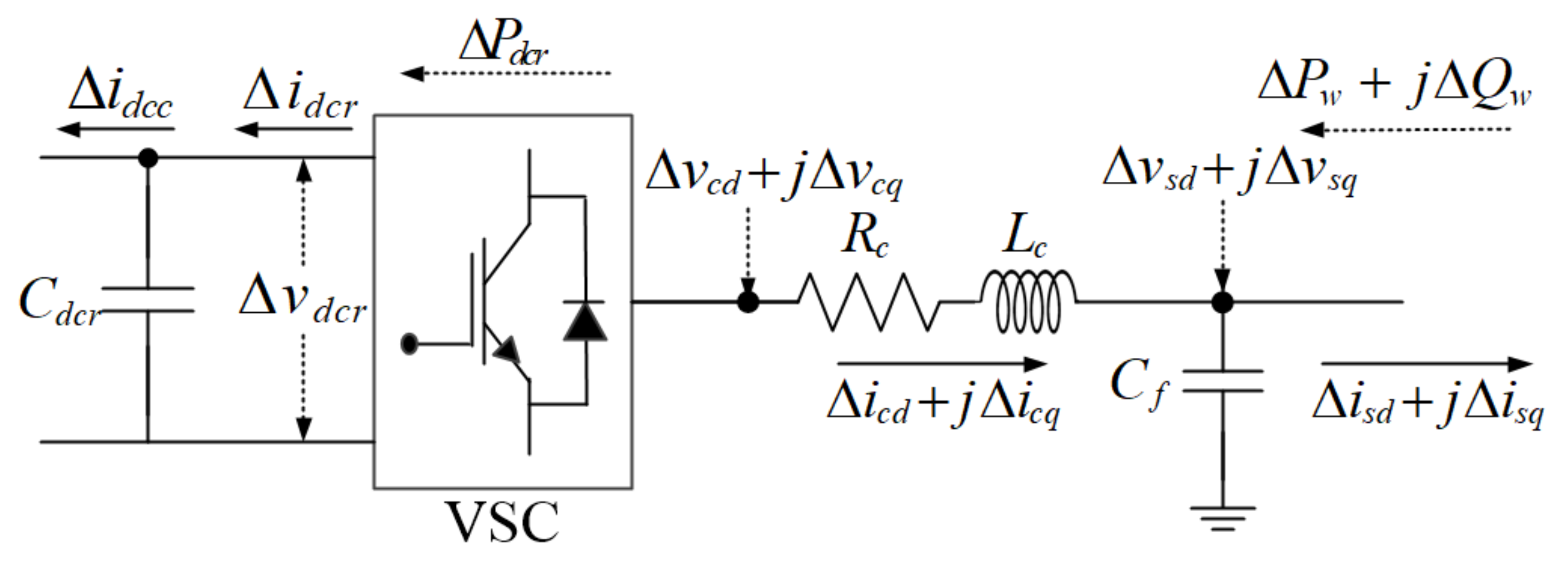
2.1. Wind Farm Side VSC Model

Figure 1 shows an ac circuit diagram of the wind farm side. All variables pertaining to voltage and current are represented in the dq-axis. The voltage and current at point of common-coupling (PCC) are represented by $\Delta v_{sd}+j\Delta v_{sq}$ and $\Delta i_{sd}+j\Delta i_{sq}$, respectively. Similarly, the voltage and current at converter side are represented by $\Delta v_{cd}+j\Delta v_{cq}$ and $\Delta i_{cd}+j\Delta i_{cq}$, respectively. The resistance and inductance between the rectifier bus and the VSC are represented by $R_c$ and $L_c$. The filter is modeled by a single capacitor of $C_f$. The dc voltage and current are represented as $\Delta v_{dcr}$ and $\Delta i_{dcr}$. From Figure 1, input variables, $\Delta P_w$ and $\Delta Q_w$, can be described in terms of voltage and current at PCC as follows:

$$\Delta P_w=-1.5(\Delta i_{sd}+i_{sd}^{*}\Delta v_{sd}),\Delta Q_w=1.5(i_{sd}^{*}\Delta v_{sq}-\Delta i_{sq}).$$

(1)

where $i_{sd}^{*}$ is the steady-state value of d-axis current at PCC. For the derivation, two assumptions are used: PCC voltages ($v_{sd}^{*}$ and $v_{sq}^{*}$) maintained their corresponding references, and q-axis current at PCC is regulated at zero.

From Figure 1, dynamic equations of converter side current, $\Delta i_{cx}$, can be described by analyzing the circuit diagram as follows:

$$s\Delta i_{cx}=-{\displaystyle \frac{R_c}{L_c}}\Delta i_{cx}+{\lambda }_x\omega \Delta i_{cy}+{\displaystyle \frac{1}{L_c}}\Delta v_{cx}-{\displaystyle \frac{1}{L_c}}\Delta v_{sx},$$

(2)

where $x\in \{d,q\}$; y is the opposite axis with x (i.e., $y=d$ when $x=q$); $\omega$ is system frequency; ${\lambda }_x$ = 1 for x = d and ${\lambda }_x$ = $-1$ for x = q. Similarly, dynamic equations of output voltages ($\Delta v_{sd}$ and $\Delta v_{sq}$) can be derived as:

$$s\Delta v_{sx}={\lambda }_x\omega \Delta v_{sy}+{\displaystyle \frac{1}{C_f}}\Delta i_{sx}-{\displaystyle \frac{1}{C_f}}\Delta i_{cx}.$$

(3)

In addition, active power transferred to dc system, $\Delta P_{dcr}$, can be represented as follows:

$$\begin{array}{cc}\hfill \Delta P_{dcr}& =-1.5(v_{cd}^{*}\Delta i_{cd}+i_{cd}^{*}\Delta v_{cd}+v_{cq}^{*}\Delta i_{cq}+i_{cq}^{*}\Delta v_{cq})\hfill \\ \hfill & =v_{dcr}^{*}\Delta i_{dcr}+i_{dcr}^{*}\Delta v_{dcr}.\hfill \end{array}$$

(4)

where $v_{cd}^{*}$, $v_{cq}^{*}$, $i_{cd}^{*}$, and $i_{cq}^{*}$ are steady-state values of corresponding variables; $v_{dcr}^{*}$ and $i_{dcr}^{*}$ are steady-state values of dc voltage and current at the VSC side. In addition, the dynamic equation of dc voltage can be represented as:

$$s\Delta v_{dcr}={\displaystyle \frac{1}{C_{dcr}}}\Delta i_{dcr}-{\displaystyle \frac{1}{C_{dcr}}}\Delta i_{dcc}.$$

(5)

Figure 2 shows the controller of wind farm side VSC. The control objective is to maintain output voltage as a constant (i.e., $\Delta v_{sd}=\Delta v_{sq}=0$). In Figure 2, to represent the hybrid MTDC system as an SS model, additional states ($\Delta u_d$ and $\Delta u_q$) are introduced, and their dynamic equations can be described as follows:

$$s\Delta u_x=-K_{ir}\Delta v_{sx},$$

(6)

where $K_{ir}$ is the integral gain of the outer-loop controller. Additionally, from the control structure in Figure 2, the reference of converter side currents ($\Delta i_{cd}^{*}$ and $\Delta i_{cq}^{*}$) can be represented as follows:

$$\Delta i_{cx}^{*}=\Delta i_{sx}+\Delta u_x-K_{pr}\Delta v_{sx}-{\lambda }_x\omega C_f\Delta v_{sy},$$

(7)

where $K_{pr}$ is the proportional gain of the outer-loop controller. By defining the inner-loop control gains as the method in [12] using the intended time constant, ${\tau }_i$, i.e., $K_{pc}=L_c/{\tau }_i$ and $K_{ic}=R_c/{\tau }_i$, dynamic equations of $\Delta i_{cd}$ and $\Delta i_{cq}$ in (3) can be rewritten as follows:

$$s\Delta i_{cx}={\displaystyle \frac{1}{{\tau }_i}}\Delta i_{cx}^{*}-{\displaystyle \frac{1}{{\tau }_i}}\Delta i_{cx}.$$

(8)

2.2. Four Terminal Dc Network Model

Figure 3 describes the 4-terminal dc network utilized in the hybrid MTDC system. The dc voltages and currents of the VSC side are represented as $\Delta v_{dcr,1}$, $\Delta i_{dcc,1}$, $\Delta v_{dcr,2}$, and $\Delta i_{dcc,2}$. Dc line is presented by $RL$-model and the parameters of dc lines are represented by $R_{dc,i}$, $L_{dc,i}$ ($i=1,2,3$). At the LCC side, smoothing reactors exploited for proper commutation are represented as $L_{s,1}$ and $L_{s,2}$. From Figure 3, dynamic equations of inverter side currents ($\Delta i_{dci,1}$ and $\Delta i_{dci,2}$) are represented as:

$$s\Delta i_{dci,k}={\displaystyle \frac{1}{L_{inv,k}}}(\Delta v_{dcr,k}-\Delta v_{dci,k}-R_{dc,k}\Delta i_{dci,k}),$$

(9)

where $k\in \{1,2\}$; $L_{inv,k}$ is the sum of $L_{dc,k}$ and $L_{s,k}$; $\Delta v_{dci,k}$ is dc voltage at the kth LCC side. Similarly, dynamic equation of dc current between two VSCs ($\Delta i_{dcn}$) can be represented as:

$$s\Delta i_{dcn}={\displaystyle \frac{1}{L_{dc,3}}}(\Delta v_{dcr,1}-\Delta v_{dcr,2}-R_{dc,3}\Delta i_{dcn}).$$

(10)

Finally, by Kirchhoff’s current law, dc currents in Figure 3 satisfy the following constraints:

$$\Delta i_{dcc,1}=\Delta i_{dci,1}+\Delta i_{dcn},\Delta i_{dcc,2}=\Delta i_{dci,2}-\Delta i_{dcn}.$$

(11)

2.3. Grid Side LCC Model

For modeling of LCC, linearized equations derived from characteristics of thyristor-based switching waveform in [13,14] are utilized, which are represented as:

$$\left[\begin{array}{c}\Delta i_{out}^R\\ \Delta i_{out}^I\\ \Delta v_{dci}\end{array}\right]=\left[\begin{array}{cccc}{D}_1& D_2& D_3& D_4\\ D_5& D_6& D_7& D_8\\ D_9& D_{10}& D_{11}& D_{12}\end{array}\right]\left[\begin{array}{c}\Delta v_{inv}^R\\ \Delta v_{inv}^I\\ \Delta i_{dci}\\ \Delta {\alpha }_i\end{array}\right]$$

(12)

where the coefficients in (14) are represented in Appendix A; real and imaginary axis values of ac voltage and current are represented by $\Delta v_{inv}^R$, $\Delta v_{inv}^I$, $\Delta i_{out}^R$, and $\Delta i_{out}^I$; firing angle of LCC is represented by $\Delta {\alpha }_i$, which can be determined by the various control methods.

2.3.1. Master–Slave Control Mode

Figure 4a describes controllers of LCC when a single LCC is operated in constant dc voltage control mode (LCC 1) and the other is operated in constant dc current control mode (LCC 2). For the LCC regulating dc voltage, an additional state ($\Delta x_i$) is introduced and the dynamic equation of it is represented as:

$$s\Delta x_i=-K_{ii}\Delta v_{dci,1},$$

(13)

where $K_{ii}$ is the integral gain of the LCC controller. In addition, $\Delta {\alpha }_{i,1}$ can be represented as:

$$\Delta {\alpha }_{i,1}=\Delta x_i-K_{pi}\Delta v_{dci},$$

(14)

where $K_{pi}$ is the proportional gain of the LCC controller. On the other hand, an additional state ($\Delta y_i$) is introduced for dc current controller and the dynamic equation of it is represented as:

$$s\Delta y_i=K_{ii}{i}_{dci,2},$$

(15)

Additionally, $\Delta {\alpha }_{i,2}$ is represented as:

$$\Delta {\alpha }_{i,2}=\Delta y_i+K_{pi}\Delta i_{dci,2}.$$

(16)

2.3.2. Voltage Droop Control Mode

Figure 4b describes controllers of LCC when multiple LCCs regulate dc voltage. For voltage droop control mode, dc reference voltage changes according to dc current. An additional state ($\Delta z_{i,p}$) is introduced and the dynamic equation of it is presented as:

$$s\Delta z_{i,p}=-K_{ii}\Delta v_{dci,p}+K_{ii}{R}_{d,p}\Delta i_{dci,p},$$

(17)

where $p\in \{1,2\}$; $R_{d,p}$ is droop coefficient of the pth LCC. In addition, $\Delta {\alpha }_{i,p}$ can be described as:

$$\Delta {\alpha }_{i,p}=\Delta z_{i,p}-K_{pi}\Delta v_{dci,p}+K_{pi}{R}_{d,p}\Delta i_{dci,p}.$$

(18)

For the modeling method of LCCs, $\Delta v_{dci,p}$ and $\Delta {\alpha }_{i,p}$ can be substituted by other state variables using (14), (16), (18), and (20). Therefore, they are not regarded as state variables in the proposed SS model.

2.4. Overall State Space Model

An overall SS model of hybrid MTDC system has 8 input variables ($\Delta P_{w,1}$, $\Delta Q_{w,1}$, $\Delta P_{w,2}$, $\Delta Q_{w,2}$, $\Delta v_{inv,1}^R$, $\Delta v_{inv,1}^I$, $\Delta v_{inv,2}^R$, and $\Delta v_{inv,2}^I$) and 19 state variables ($\Delta u_{d,1}$, $\Delta u_{q,1}$, $\Delta v_{sd,1}$, $\Delta v_{sq,1}$, $\Delta i_{cd,1}$, $\Delta i_{cq,1}$, $\Delta u_{d,2}$, $\Delta u_{q,2}$, $\Delta v_{sd,2}$, $\Delta v_{sq,2}$, $\Delta i_{cd,2}$, $\Delta i_{cq,2}$, $\Delta v_{dcr,1}$, $\Delta v_{dcr,2}$, $\Delta i_{dci,1}$, $\Delta i_{dci,2}$, $\Delta i_{dcn}$, $\Delta x_i$, and $\Delta y_i$) for master–slave control mode. For voltage droop control mode, the number of variables is equivalent with that of master–slave control, only two state variables, $\Delta x_i$ and $\Delta y_i$, are replaced by $\Delta z_{i,1}$ and $\Delta z_{i,2}$ for voltage droop control mode. Thus, overall SS model can be represented by matrix form as follows:

$$s\Delta {\mathbf{X}}_{\left[19\times 1\right]}={\mathbf{A}}_{\left[19\times 19\right]}\Delta {\mathbf{X}}_{\left[19\times 1\right]}+{\mathbf{B}}_{\left[19\times 8\right]}\Delta {\mathbf{U}}_{\left[8\times 1\right]},$$

(19)

where $\Delta \mathbf{X}$ is a state vector and $\Delta \mathbf{U}$ is an input vector. The coefficients in A and B can be derived from the equations in previous sections.

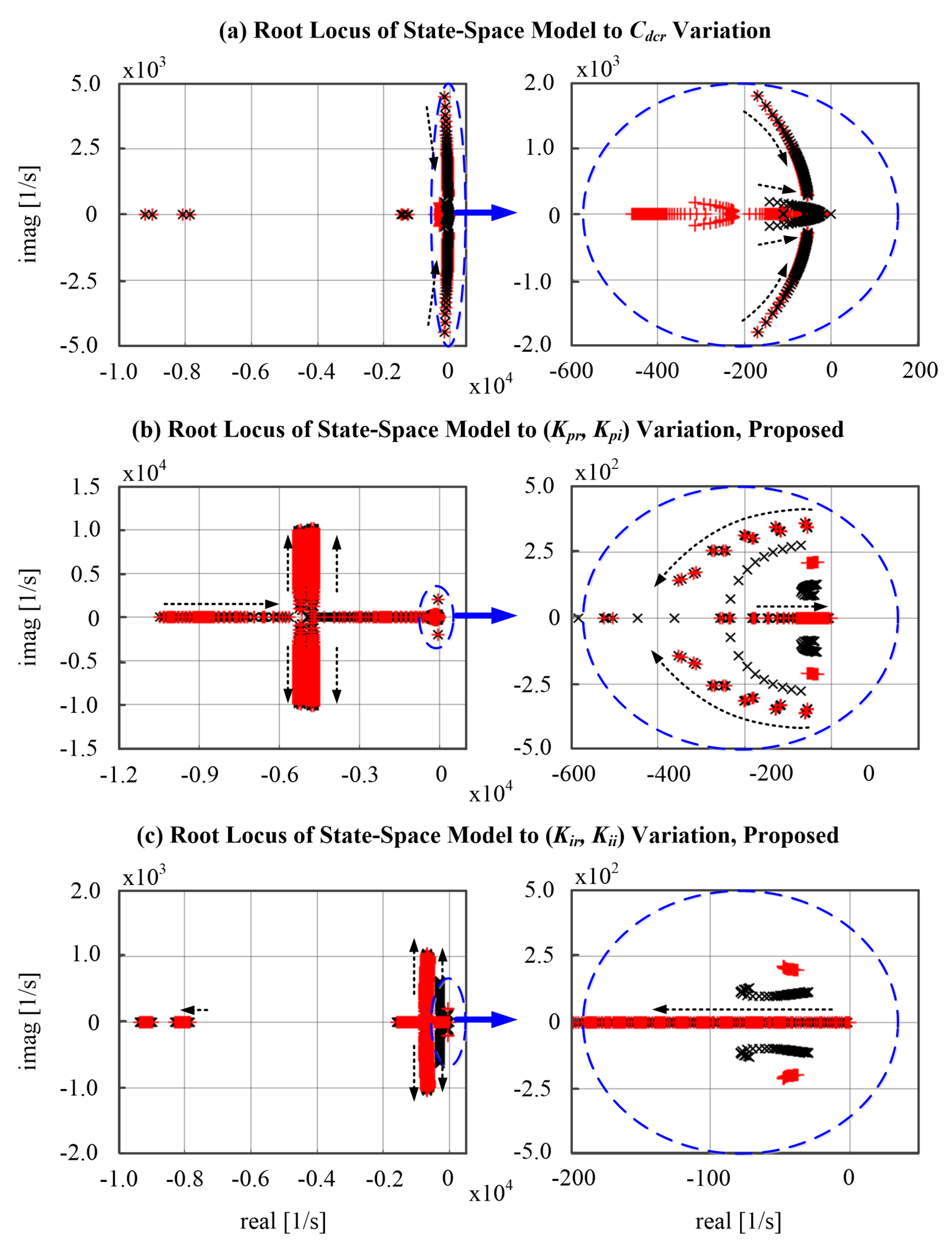
2.5. Root Locus Analysis

Figure 5 shows pole placements of SS model for two control methods: master–slave control and voltage droop control. For the stability analysis, the parameters of the hybrid MTDC system are listed in

Table 1. Parameters of the test system.

Symbol	Values	Symbol	Values
$R_{c,1}$, $R_{c,2}$	1.89 $\times {10}^{-5}$	$R_{dc,1}$, $R_{dc.2}$	0.02
$L_{c,1}$, $L_{c,2}$	4.726 $\times {10}^{-5}$	$L_{dc,1}$, $L_{dc.2}$	2 $\times {10}^{-4}$
$C_{f,1}$, $C_{f,2}$	7.935 $\times {10}^{-5}$	$R_{dc,3}$	0.004
$K_{pr}$	1	$L_{dc,3}$	4 $\times {10}^{-5}$
$K_{ir}$	100	$K_{pi}$	0.63
${\tau }_i$	1 $\times {10}^{-4}$	$K_{ii}$	41.3386
$P_{w,1}$	0.5	$P_{w,2}$	0.7
$C_{dcr,1}$, $C_{dcr,2}$	0.0125	$L_{s,1}$, $L_{s,2}$	0.002
$R_{d.1}$	0.1	$R_{d,2}$	0.1

[15,16]. In Figure 5, all poles for both methods are located in the left half-plane; the hybrid MTDC system can be operated in stable range regardless of control methods at given parameters. Specifically, single pole in real axis is located closer to vertical axes when master–slave control method is utilized as shown in the enlarged part of Figure 5. Therefore, for identical operating point, stability margin increases with adopting voltage droop control for the hybrid MTDC system.

Additionally, root-locus analysis is provided with variations in $C_{dcr}$, ($K_{pr}$, $K_{pi}$), and ($K_{ir}$, $K_{ii}$). Specifically, in Figure 6, $C_{dcr}$, ($K_{pr}$, $K_{pi}$), and ($K_{ir}$, $K_{ii}$) are increased from 0.0025 to 0.1, (0.1, 0.063) to (10, 6.3), and (10, 4.13) to (1000, 413), respectively. These maximum and minimum boundaries were determined based on [14,15]. As shown in Figure 6, the trajectory of the poles is always in the left-hand half plane with variations in parameters. In other words, a stable operation of the hybrid MTDC system in guaranteed over a wide range of parameter values using the proposed SS model.

3. Grid Monitoring and Fault Localization Method

3.1. Cable System Modeling

Before applying the fault localization method to the MTDC system, we design the equivalent RLCG circuit model based on the experimental results [11]. Through the comparison analysis between the reflected signal from the 7 m length of the actual HTS cable and from the equivalent circuit model using simulation, we model the equivalent circuit of the HTS cable [11]. As shown in Figure 7, we apply the step pulse to the 7 m length of HTS cable and acquire the reflected signal from the cable termination. Parameter values of equivalent circuit were tuned to match the simulation results with the results obtained in the experiment. Figure 7a illustrates the experimental setup and the comparison analysis between the simulation and experimental results are shown in Figure 7b. Since the acquired signals from the simulation and from the experiment are matched as shown in Figure 7b, it can be determined that the equivalent circuit modeling has been successfully performed. Based on the modeling of the HTS cable, we design the basic structure of MTDC system as seen in Figure 8. The configuration of 4-terminal dc network model, as seen in Figure 3, can be modeled as specified length and parameter value as shown in Figure 8.

The proposed MTDC system consists of 5 cable sections as shown in Figure 8. Figure 9 and Figure 10 show the equivalent circuit modeling of MTDC system of failure conditions.

As shown in Figure 8, cable sections are numbered in order. The lengths of cable sections are set as follows: $\#1$ cable: 20 km, $\#2$ cable: 40 km, $\#3$ cable: 20 km, $\#4$ cable: 20 km, #5 cable: 20 km. This paper simulates a variety of scenarios of failure situations as follows: scenario 1: normal condition, scenario 2: failure condition (fault position at 5 km in cable Section 2), and scenario 3: failure condition (fault position at 5 km in cable Section 3). The distance from the start point of cable Section 1 to fault location in scenario 2 and in scenario 3 is equal to 25 km. Since the proposed system has branch points, it is difficult to detect the fault position using conventional reflectometry method.

3.2. Fault Localization Based on Reflectometry Method

3.2.1. Time Frequency Domain Reflectometry Method

In this paper, we use the time–frequency domain reflectometry (TFDR) to detect the fault position. TFDR is a kind of reflectometry method using a time–frequency analysis. The basic theory of reflectometry can be described using Figure 11. We apply the incident signal to target cable, and the reflected signal is generated from the impedance mismatch point, such as fault and termination. Figure 11 shows the signal path through a 100 km long cable containing the fault. The reflection coefficient, $\Gamma$ can be written as follows:

$$\begin{array}{c}\hfill \Gamma =\frac{Z_L-Z_C}{Z_L+Z_C}=\frac{V_r}{V_i}\end{array}$$

(20)

where $Z_L$ is the fault impedance, $Z_C$ is the characteristic impedance, $V_r$ and $V_i$ are the voltages of incident and reflected signals, respectively. Based on the reflection coefficients, the reflected signals, which are generated at fault location and termination, can be acquired at the signal injection point. The round trip time of reflected signal can be converted into the distance from the signal injection point to impedance mismatch location as shown in Figure 11.

In TFDR, we use the Gaussian linear chirp signal as the incident signal, and the incident signal is represented as follows [10]:

$$s\left(t\right)=\left\{\begin{array}{cc}{\left(\frac{\alpha }{\pi }\right)}^{1/4}·e^{-\alpha {(t-t_0)}^2/2+j(\beta {(t-t_0)}^2/2+{\omega }_0(t-t_0))},\hfill & \mathrm{t}=0\le \mathrm{t}\le T\hfill \\ 0,\hfill & \mathrm{otherwise}.\hfill \end{array}\right.$$

where T is the duration of the incident signal, A is the amplitude, $\alpha ,\beta ,t_0$, and ${\omega }_0$ determine the time duration, frequency sweep rate, time center, and frequency center. In TFDR, the reference signal can be designed to fit the frequency characteristics of the target cable and the detection range, and there are three parameters that can be designed as follows: center frequency, frequency bandwidth, and time duration [11]. The reflected signal is expressed as follows:

$$\begin{array}{c}\hfill r(t-d)=\eta ·{\left(\frac{\alpha }{\pi }\right)}^{1/4}·e^{-\alpha {(t-t_d)}^2/2+j(\beta {(t-t_d)}^2+{\omega }_0(t-t_d)+\varphi )}\end{array}$$

(21)

where $\eta$ is the magnitude of the attenuation coefficient at the traveling distance, and $t_d$ is the time delay of the reflected signal. Since we acquire a signal in which the applied signal and the reflected signal are mixed, TFCC is used to detect the reflected signal among the mixed signals. Wigner–Ville transform is a transformation tool for analyzing the characteristics of signal in the time and frequency domain. TFCC is calculated by using the Wigner–Ville distribution and Wigner–Ville is expressed as follows [10]:

$$\begin{array}{c}\hfill W(t,w)=\frac{1}{2\pi }\int s(t+\tau /2)s^{*}(t-\tau /2)e^{-jw\tau }d\tau \end{array}$$

(22)

Then, the Wigner distribution of the reference signal $W_s(t,w)$ is derived as follows:

$$\begin{array}{c}\hfill W_s(t,w)=\frac{1}{\pi }{e}^{-\alpha {(t-t_0)}^2-{(w-\beta (t-t_0)-w_0)}^2/\alpha }\end{array}$$

(23)

Based on the Wigner–Ville distribution, we detect the reflected signal from the incident signal using the similarities between incident and reflected signal, because the Wigner–Ville distribution is a kind of energy distribution. The normalized TFCC can be written as follows:

$$\begin{array}{c}\hfill C_{sr}\left(t\right)=\frac{2\pi }{E_s{E}_r}\int \int W_r(t^{\prime },w)W_s(t^{\prime }-t,w)dwd{t}^{\prime }\end{array}$$

(24)

where $E_r$ and $E_s$ are energy of reflected and incident signal, respectively. Using the normalized TFCC, we can obtain the fault distance between defect and signal injection point.

3.2.2. Fault Localization Method on Branch Cable System

Based on the proposed reflectometry method, we can derive the distance between the signal injection point and fault location. However, information from that distance cannot specify in which section the defect is located. As a result of this point, the conventional reflectometry is difficult to apply to a branch cable system. Using that distance derived from each signal injection point, we can specify the faulty section and localize the defect in the following Algorithm 1.

Algorithm 1: Fault Localization Algorithm.

if $d_i>L_i$   find $L_i+L_j-d_i=d_j$    the fault is located $d_j$ km from     the j th section starting point.   else    the fault is located $d_i$ km from    the i th section starting point.  end

where $d_i$ and $L_i$ are the distance from the ith section termination and impedance discontinuity point and the ith section length, respectively. The distance obtained by using the reflected signal acquired from a section other than the corresponding section will be greater than the length of each section. For example, if the defect is located in the Section 2, the distance derived from the Section 1 and Section 3 will be greater than the length of Section 1 and Section 3. From the point of view of Section 1, it can be determined that the fault occurred in Section 2 or Section 3, because the measured distance of failure is longer than the length of the corresponding section. The same is true of Section 3’s point of view. If the obtained fault distance in a section is longer than the length of the section, then find a section where the result of the sum of the fault distances measured in the other section and that section is equal to the sum of the lengths of both sections. The case of multiple faults is not covered in this paper, and multiple reflection signals generated from multiple faults will be studied in the future. The branch cable system can be monitored using the proposed algorithm above, and the performance was verified through simulation in the next section.

4. Discussion

4.1. Operation Control Results

Figure 12 compares the step responses of wind power ($P_{w,1}$ and $P_{w,2}$), dc current at inverter side ($i_{dci,1}$ and $i_{dci,2}$), and dc voltage at inverter side ($v_{dci,1}$ and $v_{dci,2}$) between the proposed SS model using the master–slave control versus the voltage droop control.

At $t=1s$, active power of wind farm 1, $P_{w,1}$, decreases from 0.5 to 0.4 p.u. as shown in Figure 12a. In Figure 12b,c, for master–slave control method, dc voltage of VSC 1, $v_{dci,1}$, and dc current of VSC 2, $i_{dci,2}$, are maintained as a constant regardless of active power deviation. Meanwhile, only current at VSC 1 changes according to active power variation. On the other hand, dc voltage and currents for voltage droop control method change together with active power deviation as shown in Figure 12b,c. In addition, power sharing ratio between two VSCs is almost unity as two droop coefficients are identical as described in Table 1. In other words, the characteristics of voltage droop control method can be reflected in the proposed SS model for the hybrid MTDC system.

4.2. Fault Localization Results

Fault localization results according to each scenario are shown in Figure 13, Figure 14 and Figure 15. Each figure consists of two parts: acquired signal and TFCC results. The reflected signals, which are current signal, can be acquired through the current sensor. Figure 13b illustrates the current 0, current 1, current 2, current 3, and current 4 which are the signals acquired from the start point of Section 1, from the end point of Section 1, from the start point of Section 2, from the end point of Section 4, and from the start point of Section 5 as shown in Figure 8. The scenario 1, called a normal condition, is depicted in Figure 8. To explain the TFCC results in order, we can confirm that the TFCC of current has peak values at 0 km, 20 km, and 40 km. Peak position of the TFCC graph indicates the impedance discontinuity point, such as fault, termination, and joint. In this case, the reflected signal generated from the end point of Section 1 and the mixed signal with the reflected signal from the end point and second reflected signal at the end point of Section 1 are plotted at 20 km and 40 km in sequence. TFCC graph colored in black, which is acquired through the current sensor 1, detects the impedance discontinuity points located at 10 km and 30 km. The location of impedance discontinuities point means the distance to the acquisition point after the traveling signal is reflected from the impedance discontinuities point, and the origin point is the signal injection point, respectively. However, the peak located at 10 km of current 1 graph indicates a transmitted distance of applied signal between the origin point and current sensor 1. The distance of reflected signal can be calculated as follows: $Distance=\frac{V.O.P\times T.O.A}{2}$, where $V.O.P$ and $T.O.A$ refer the velocity of propagation and time of arrival. In comparison with it, the transmitted distance of signal can be derived as: $Distance=V.O.P\times T.O.A$. As the purpose of this paper was to find the impedance discontinuities position, the distance on the x-axis of TFCC graph is calculated based on the distance of the reflected signal. The peak located at 30 km of TFCC graph in current 1 refers to the distance from the point at which the transmitted signal was acquired by the current sensor 1, 10 km, and the return path of the reflected signal from the branch point of Section 4 and Section 5. In this manner, we can analyze the rest of the TFCC graphs in scenario 1. Both Figure 7 and Figure 14 illustrate the modeling of the MTDC system and TFCC results in Figure 14. The common thing of TFCC results of Figure 14 and Figure 15 is a fault distance between the origin point and the fault location, and this makes it difficult to detect the fault location of the cable including the branch point. In this case, we first make a list of faulty cable sections based on the derived distance from the origin point. Then, we analyze the TFCC results acquired from adjacent instruments at the branch point of suspected faulty cable section. The difference between TFCC results of Figure 14 and Figure 15 can be found through the TFCC results acquired from current sensors 2 and 3. The difference between TFCC results can tell you which cable section the fault position is located in for a branch situation.

Figure 16 shows the TDR results in scenario 1 to comparatively analyze the results of the proposed method. The reflected signal in TDR has different phase depending on whether it is open or short at the impedance mismatch point. According to reflection coefficients, the sign of reflected signal has a positive value at open fault, like cable termination. In the case of short fault, the sign of it has a negative value. The $V.O.P$ of step pulse can be calculated using the transmitted distance between voltage source and current sensor 1, 10 km. The waveform obtained by current sensor 1 suddenly increased at 10 km and decreased sharply at 30 km and 50 km. The distance from the voltage source to the current sensor 1 is 20 km, but the distance in the Figure 16 is 10 km because it is the result of dividing by 2 like calculating the round trip distance. In addition, a sudden change is observed at 30 km and 50 km by adding the 20 km and 40 km long cable in Section 2 and Section 3. The reason that the waveform observed by the current sensor 3 is reversed is because the current sensor 3 is connected opposite the direction of the current. As shown in Figure 16, the signal is distorted along the distance with dispersion. The dispersion of the signal widens the point of change of the signal to the range rather than an exact location. It can be seen that after about 30 km in the graph, the range of change expands to a range of 10 km, which means that the estimated distance error of fault location using TDR can reach 10 km. In contrast, the proposed method can accurately calculate the fault location, and it is easy to make it as an automated algorithm because the fault location can be calculated through the peak point without complex waveform analysis.

5. Conclusions

We propose an MTDC operation solution that integrates an operation control scheme and a fault localization algorithm in case of failure. (1) Modeling methods of hybrid MTDC system featuring two control methods, master–slave control and voltage droop control, are proposed in this paper. We first show the procedure to derive SS models of the hybrid MTDC model with two control schemes. In addition, we investigated the stability of hybrid MTDC systems and compared two control methods by using root-locus analysis. Finally, the time-domain simulations were provided using two SS models and the results suggested that the proposed modeling methods represent well the hybrid MTDC system with two control methods. By using the proposed SS model and comparing pole trajectories of two methods, guidelines to determine the control scheme on the hybrid MTDC system can be suggested. (2) We model the equivalent circuit of the hybrid MTDC system based on the comparison analysis between the simulation results and experimental results of 7 m HTS cable. We propose a TFDR system for applying the target MTDC system, which has multiple branch points, and verify the performance of the fault localization method through simulation results.

References

1. Wu, Y.; Su, P.; Su, Y.; We, T.; Tan, W. Economics- and reliability-based design for an offshore wind farm. IEEE Trans. Ind. Appl. 2017, 53, 5139–5149. [Google Scholar] [CrossRef]
2. Hou, P.; Hu, W.; Soltani, M.; Chen, C.; Zhang, B.; Chen, Z. Offshore wind farm layout design considering optimized power dispatch strategy. IEEE Trans. Sustain. Energy 2017, 8, 638–647. [Google Scholar] [CrossRef]
3. Wang, L.; Wang, K.; Lee, W.; Chen, Z. Power-flow control and stability enhancement of four parallel-operated wind farms using a line-commutated HVDC link. IEEE Trans. Power Deliv. 2010, 25, 1190–1202. [Google Scholar] [CrossRef]
4. Karaagac, U.; Mahseredjian, J.; Cai, L.; Saad, H. Offshore wind farm modeling accuracy and efficiency in MMC-based multiterminal HVDC connection. IEEE Trans. Power Deliv. 2017, 32, 617–627. [Google Scholar] [CrossRef]
5. Bianchi, F.D.; Garciá, J.L.D. Coordinated frequency control usint MT-HVDC grids with wind power plants. IEEE Trans. Sustain. Energy 2016, 7, 213–220. [Google Scholar] [CrossRef]
6. Preece, R.; Milanović, J.V. Tuning of a damping controller for multiterminal VSC-HVDC grids using the probabilistic collocation method. IEEE Trans. Power Deliv. 2014, 29, 318–326. [Google Scholar] [CrossRef]
7. Li, C.; Zhan, P.; Wen, J.; Yao, M.; Li, N.; Lee, W. Offshore wind farm integration and frequency support control utilizing hybrid multiterminal HVDC transmission. IEEE Trans. Ind. Appl. 2014, 50, 2788–2797. [Google Scholar] [CrossRef]
8. Han, M.; Xu, D.; Wan, L. Hierarchical optimal power flow control for loss minimization in hybrid multi-terminal HVDC transmission system. CSEE J. Power Energy Syst. 2016, 2, 40–46. [Google Scholar] [CrossRef]
9. Li, Z.; Zhan, R.; Li, Y.; He, Y.; Hou, J.; Zhao, X.; Zhang, X. Recent developments in HVDC transmission systems to support renewable energy integration. Glob. Energy Interconnect. 2018, 1, 595–601. [Google Scholar]
10. Chang, S.J.; Park, J.B. Wire mismatch detection using a convolutional neural network and fault localization based on time–frequency-domain reflectometry. IEEE Trans. Ind. Electron. 2019, 66, 2102–2110. [Google Scholar] [CrossRef]
11. Chang, S.J. Advanced signal sensing method With adaptive threshold curve based on time frequency domain reflectometry compensating the signal attenuation. IEEE OJ. Trans. Ind. Electron. 2020, 1, 22–27. [Google Scholar] [CrossRef]
12. Guo, Y.; Gao, H.; Wu, Q.; Zhao, H.; Østergaard, J.; Shahidehpour, M. Enhanced voltage control of VSC-HVDC-connected offshore wind farms based on model predictive control. IEEE Trans. Sustain. Energy 2018, 9, 474–487. [Google Scholar] [CrossRef] [Green Version]
13. Karawita, C.; Annakkage, U. Multi-infeed HVDC interaction studies using small-signal stability assessment. IEEE Trans. Power Deliv. 2009, 24, 910–918. [Google Scholar] [CrossRef]
14. Wang, L.; Thi, M. Comparisons of damping controllers for stability enhancement of an offshore wind farm fed to an OMIB system through an LCC-HVDC link. IEEE Trans. Power Syst. 2013, 28, 1870–1878. [Google Scholar] [CrossRef]
15. Trinh, N.; Zeller, M.; Wuerflinger, K.; Erlich, I. Generic model of MMC-VSC-HVDC for interaction study with ac power system. IEEE Trans. Power Syst. 2016, 31, 27–34. [Google Scholar] [CrossRef]
16. Faruque, M.; Zhang, Y.; Dinavahi, V. Detailed modeling of CIGRE HVDC benchmark system using PSCAD/EMTDC and PSB/SIMULINK. IEEE Trans. Power Deliv. 2005, 21, 378–387. [Google Scholar] [CrossRef]
Figure 1. Configuration of the wind side ac circuit.
Energies 14 01292 g001
Figure 2. Controller of wind farm side voltage-source converter (VSC).
Energies 14 01292 g002
Figure 3. A configuration of a 4-terminal dc network model.
Energies 14 01292 g003
Figure 4. A control scheme of grid side LCCs in (a) master–slave control mode and (b) voltage droop control mode.
Energies 14 01292 g004
Figure 5. Pole placement of the proposed state-space (SS) model.
Energies 14 01292 g005
Figure 6. Eigenvalue locations for the proposed method with (a) C d c r increasing from 0.0025 to 0.1; (b) ( K p r , K p i ) increasing from (0.1, 0.063) to (10, 6.3); and (c) ( K i r , K i i ) increasing from (10, 4.13) to (1000, 413).
Energies 14 01292 g006
Figure 7. High temperature superconducting (HTS) cable modeling. (a) Experimental setup (b) Experimental resulets of modeling HTS cable.
Energies 14 01292 g007
Figure 8. Equivalent circuit modeling of multi-terminal high-voltage direct-current (MTDC) system: scenario 1.
Energies 14 01292 g008
Figure 9. Equivalent circuit modeling of MTDC system: scenario 2.
Energies 14 01292 g009
Figure 10. Equivalent circuit modeling of MTDC system: scenario 3.
Energies 14 01292 g010
Figure 11. The basic conceptual diagram of reflectometry.
Energies 14 01292 g011
Figure 12. The responses of the hybrid MTDC systems for the stepped wind power change using the two control methods: master–slave control and voltage droop control. (a) Wind power at VSC sides, P w ; (b) dc current at inverter side, i d c i ; and (c) dc voltage at inverter sides, v d c i .
Energies 14 01292 g012
Figure 13. Fault localization results: scenario 1.
Energies 14 01292 g013
Figure 14. Fault localization results: scenario 2.
Energies 14 01292 g014
Figure 15. Fault localization results: scenario 3.
Energies 14 01292 g015
Figure 16. Fault localization results using TDR: scenario 1.
Energies 14 01292 g016