A Methodology for the Enhancement of the Energy Flexibility and Contingency Response of a Building through Predictive Control of Passive and Active Storage

Abstract

Optimal management of thermal energy storage in a building is essential to provide predictable energy flexibility to a smart grid. Active technologies such as Electric Thermal Storage (ETS) can assist in building heating load management and can complement the building’s passive thermal storage capacity. The presented paper outlines a methodology that utilizes the concept of Building Energy Flexibility Index (BEFI) and shows that implementing Model Predictive Control (MPC) with dedicated thermal storage can provide predictable energy flexibility to the grid during critical times. When the utility notifies the customer 12 h before a Demand Response (DR) event, a BEFI up to 65 kW (100% reduction) can be achieved. A dynamic rate structure as the objective function is shown to be successful in reducing the peak demand, while a greater reduction in energy consumption in a 24-hour period is seen with a rate structure with a demand charge. Contingency reserve participation was also studied and strategies included reducing the zone temperature setpoint by 2${}^{\circ }$C for 3 h or using the stored thermal energy by discharging the device for 3 h. Favourable results were found for both options, where a BEFI of up to 47 kW (96%) is achieved. The proposed methodology for modeling and evaluation of control strategies is suitable for other similar convectively conditioned buildings equipped with active and passive storage.

1. Introduction

As the global focus to decrease Greenhouse Gas (GHG) emissions continues, the demand for cleaner electricity is increasing; however, this promising development puts a strain on electric grids. Recently, utility grids have been incorporating clean renewable energy generating resources such as photovoltaics (PV) or wind turbines. However, this increase in intermittent production results in a supply side that has a variable output, creating new challenges for utilities and electricity customers.

One major challenge linked to integrating distributed renewable energy sources into utility grids is that times of high consumption from buildings rarely correspond with the power generation from these intermittent renewable sources. Periods of peak consumption from buildings (morning and evening for residential and afternoon for commercial) do not match the time of greatest solar generation, which occurs midday, as depicted by the well-known illustration of the “duck curve” [1]. Similar supply–demand mismatch issues are observed elsewhere, although for different reasons (for instance in heating dominated regions).

Demand side management and Demand Response (DR) programs are popular approaches to incentivize electricity customers—often building owner/operators—to alter their electricity demand during critical times for the grid.

The concept of energy flexibility has received significant attention in recent years. It is useful to estimate the amount of energy flexibility that a building can provide to the grid, since activation of this flexibility can help alleviate the grid’s strain when the demand approaches exceed what the grid can safely supply. The International Energy Agency Energy in Buildings and Communities Programme’s (IEA EBC) Annex 67 introduced the notion of “Energy Flexible Building”, defined by the Annex as “a building able to manage its demand and generation in accordance with local climate conditions, user needs, and grid requirements” [2].

Building control can take advantage of thermal mass to shift power consumption from one critical period to another. Different end-uses can be rescheduled before or after a specific period without adverse impact, such as a reduction of thermal comfort. We can think also of specific systems within Heating, Ventilation, and Air Conditioning (HVAC) (active thermal storage or batteries) or embedded in the building—such as heavy radiant floors—that can be used to shift energy consumption without affecting occupant comfort. When coordinating these different systems, future or expected needs, availabilities, and constraints that may depend on occupant activity schedule, weather, grid state, day in week, etc. must be considered. Model predictive control is an optimal tool to achieve this.

The most relevant application of energy flexibility is demand response during peak periods of the grid. A Building Energy Flexibility Index (BEFI) could be used to quantify potential participation of a customer for such a demand response event. A preliminary introduction and description of the concept of a BEFI with case studies can be found in two previous conference papers on the topic [3,4].

Over 99.8% (37.3 GW) of the electric power is generated by hydroelectric plants in Québec, Canada [5], and commercial buildings in this region often use electricity as their main or only energy source. An abundance of stable generation has resulted in low electricity rates and elevated fuel prices with limited gas distribution in certain areas. During very cold winter days, a heavy demand on the grid is observed and is partially due to space heating peak loads. About 9% of the province’s winter peak load is associated with heating in commercial and institutional (C & I) buildings [6]; thus, C & I buildings represent a considerable amount of the electric load in the province. Due to these mentioned issues related to peak demand, there is increasing activity in quantifying the energy flexibility of buildings and increasing participation demand response programs.

It is possible (and worthwhile) to consider optimization of the entire electric energy system, not only the grid. This electric system spans from the generation units to the final customer end-uses. Buildings are part of this system as end-uses and can contribute to the energy flexibility of the electric system. Building science and advanced controls must be applied to help make this energy flexibility available to the grid. This study incorporates the concept of an energy flexible building and the use of Model Predictive Control (MPC) for buildings in cold climate regions with thermal storage as a dispatchable storage medium.

A notable feature of some Québec commercial customer rates is that each monthly bill throughout the year can be affected by the building’s highest winter demand. The minimum monthly electric billing demand is set at 65% of the peak power reported during the winter months. Thus, appropriate consideration should be given to the demand management strategies of a building during winter since it can affect the bills over the year.

Other fields such as electrical engineering and chemical processing have a well-established MPC domain for control techniques [7], while MPC has been shown to be a promising strategy for improved operation in buildings [8,9,10]. It has yet to be adopted for widespread implementation in real buildings, though it has received rising attention in buildings research.

MPC is a multi-variable control method that incorporates several additional aspects with the controller: a dynamic model of the system to be controlled, forecasts of future disturbances such as weather, a cost function that is minimized over a prediction horizon, and sometimes a history of past control sequences. The basis of MPC in buildings is that better control of the building energy systems and planning of resources is possible due to insights into forecast weather, expected occupancy, and the thermal response of the building. For example, better management could be achieved through MPC of thermal storage capabilities through better planning of when to store or use the stored thermal energy.

Optimization of building control sequences can become complicated due to the number of variables and constraints that considered. The construction of a suitable building control model is a central step for successful MPC. As each thermal model is often designed for a specific building, the level of effort needed to create a model can be significant and difficult to determine in advance. Expert engineering judgment and heat transfer knowledge are paramount for the development of adequate building thermal models for MPC, such as an understanding of what physical details are important to include or omit in the model.

Several modeling software are appropriate for studying MPC in buildings. Some advantages and disadvantages have been discussed by [11], where they compare Modelica and MATLAB. However, one missing piece in the area of MPC and building controls is a practical way to visualize and quantify the effects that advanced controls have on building operation and energy use, which hampers efficient transfer of research developments to a wider audience.

This study aims to evaluate the energy flexibility potential of a zone equipped with a dedicated thermal storage device. One aim is to match stored thermal energy in a dedicated storage device to the zone heating energy demand for the following day. To achieve this, an estimate of the heat requirements of the conditioned zone for the following day are needed and optimal controls through model predictive control (MPC) are evaluated. Prediction uncertainties due to model parameter identification and weather forecasts are also considered.

2. Literature Review—Enhanced Flexibility Through Optimal Control

Building load flexibility can be described as a building’s capability to modify its energy demand at a specific time by postponing or shifting consumption when compared to a reference scenario (business as usual). Incorporating the principles of building energy flexibility together with on-site energy storage devices and advanced or optimized control strategies is essential for optimizing energy consumption and matching demand with the availability of energy from the grid at critical times [12,13]. In recent years, various international studies on the quantification and utilization of building energy flexibility have been conducted, and there is now a breadth of published work in this relatively newly defined area [2].

The adjustability or flexibility of a building’s heating and/or cooling system has been the topic of many studies, some of which will be described in the following paragraphs. In general, these studies studied the impact of Demand Side Management (DSM) strategies at the building level or at the energy infrastructure level.

Several studies have looked at the energy flexibility potential of a single building. Le Dréau and Heiselberg [14] assessed the potential of residential buildings to regulate heating power and to identify strategies to capitalize on flexibility potential. Hurtado et al. [15] proposed a method to quantify the demand flexibility potential of individual buildings. They assessed the effects on demand flexibility from weather fluctuations, construction variations, and comfort consideration. Other researchers have concluded that specific technologies and parametric optimizations are needed to maximize energy flexibility in residential buildings, such as Wei et al. [16], who found that, for buildings in Austria built after 1980, 50% of peak loads from space heating can be shifted to off-peak times.

Other studies have considered a group of buildings together and the potential aggregated energy flexibility. Vigna et al. [17] expanded the study of energy flexibility on a single building to a cluster of buildings. This approach capitalizes on the disparities in energy consumption patterns between different building types and management of load shifting. Foteinaki et al. [18] investigated the potential for flexibility of low-energy buildings and analyzed the thermal storage capacity present in the structural mass. The study showed that low-energy buildings can remain autonomous for several hours and that, when many buildings are aggregated together—rather than a standalone building—the flexibility becomes considerable.

Effective advanced control strategies harness the thermal inertia inherently present in the structural components of a building and coordinate the operation of different systems such as thermal storage, electrical storage, on-site renewables, and heat pumps [19,20,21]. The fluctuations in weather and occupancy directly affect the operation of a building, which can result in significant load variations between daytime and nighttime and thus large demand variations. To manage these fluctuations, proper energy management and solid knowledge of the dynamic behaviour of buildings is of the utmost importance.

2.1. Improving Energy Flexibility in Buildings

Energy flexible buildings, through smart DSM, smart DR, and the incorporation of efficient energy storage, are one of the most encouraging prospects to roll-out storage and renewable technologies on a large scale in existing electricity networks.

From field study data, Aduda et al. [22] demonstrated that office buildings can adequately provide power flexibility for the grid. However, estimation of the demand-side flexibility potential may be difficult due to variations in indoor air quality and thermal comfort in different zones within a building.

In a study by Sánchez Ramos et al. [23], demand management measures were analyzed by using the buildings’ thermal mass as thermal storage. Cost savings of 3.2% for heating and 8.5% for cooling were observed after the implementation of new control strategies for demand management. Twice the amount of savings were seen when a building was previously refurbished. They concluded that low installation costs make these measures viable if regional electric pricing and user behaviour allow for adequate flexibility.

Perez et al. [24] investigated the ability of individual residential customers to lower peak demand at the community level. Their proposed integrated control and scheduling was found to minimize the peak demand for the neighborhood by taking advantage of individual preferences and physical differences between houses (i.e., insulation values, window type, how many floors, orientation, etc). A reduction of one-quarter of the daily peak load was achieved for a group of houses when compared with the reference case of individually controlled thermostats and appliances.

Sharma et al. [25] presented a model for optimal energy management of a residential building. They proposed centralized energy management system (CEMS), where optimized decisions were determined by considering realistic model parameter settings and customer preferences. The proposed CEMS reduced both the energy cost and energy consumption of the customers over a day.

Patteeuw et al. [26] investigated how the participation of residential heat pumps in load shifting could help reduce operational costs and CO₂ emissions and how homeowners with heat pumps could be motivated to achieve benefits from flexibility measures. Operation during dynamic time-of-use (TOU) pricing performed better; however, dynamic TOU showed poorer outcomes at high levels of residential heat pump penetration.

2.2. Predictive Building Load Management and Model Predictive Control (MPC)

Model predictive control and its potential to improve the operation of buildings has been abundantly illustrated over the last couple decades [27,28,29,30,31,32]. Often, MPC studies have concentrated on the operation of dedicated energy storage, mostly focusing on cooling applications and typically subjected to TOU rates [33]. Moroşan et al. [34] looked at a multi-zone building and studied the efficacy of joining decentralized and centralized control operations. Information was exchanged at each time step, and good control performance and low computational times were achieved. Another demonstration of distributed rather than centralized MPC was found in Hou et al. [35], where it was implemented in a real building.

Huang et al. [36] investigated robust MPC, which integrates uncertainty to improve the stability of MPC but found that the additional computational burden impeded performance and practicality. Jorissen and Helsen [37] recognized the challenges of developing the required model of each building for an MPC controller and that significant expert knowledge is often required for proper building thermal model development. Jorissen and Helsen [37] suggested a “Linear Automated Toolchain for MPC” (LAT-MPC) that permits a high degree of automation for controller model development and running MPC.

Sturzenegger et al. [8] showed a successful case of implementing MPC for 3 months in a real office building located in Switzerland. Data showed that adequate comfort levels for occupants were maintained, and this suggested that the MPC performance was greater compared to the original strategy.

3. Methodology

Data-driven reduced-order thermal models (ROMs) for different archetype zones and system configurations are useful tools to identify strategies for developing and quantifying energy flexibility in the building–grid interaction. These models, which account for thermal mass and the inherent thermal delay, are typically first- to third-order Resistance–Capacitance (RC) thermal networks and can be calibrated with smart meter and weather data or more detailed data from building automation systems (BAS) and smart thermostats.

An MPC-based simulation was carried out to estimate the heat requirements of the conditioned zone for the following day and to identify optimal controls for the thermal storage device at a zone temperature setpoint schedule. Several simulation studies were carried out to further evaluate the versatility of the identified schedules, while different weather conditions, control horizons, and cost functions were evaluated.

This study was carried out in the following steps, as shown in Figure 1:

• Real building measurement data were collected from the BAS. Data included variables such as building power kW, zone air temperature, weather data, and specific data related to the ETS in question. Data were collected at 15-minute intervals.
• Numerical thermal building or device control-oriented models were developed. These models are physics-based ROM grey-box RC thermal networks. These models were then calibrated using the collected data from the first step. Critical parameters were identified using the gradient descent-based optimization function fmincon in MATLAB. A detailed explanation of the model development process for the ETS device is found in [4,38,39].
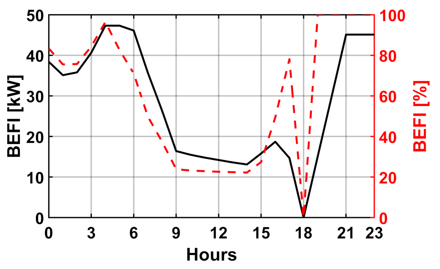
• Predictive control strategies for very cold days were identified for optimized peak load management and building energy flexibility by quantifying the BEFI depending on when a signal from the utility is given to the building owner. A heuristic approach was compared to optimized control MPC using fmincon in MATLAB. See Appendix A for further details on the developed BEFI.
• Shoulder season MPC studies were also performed with the goal of improving the operation of the ETS to reduce energy consumption by storing the appropriate amount of energy needed for a warmer shoulder season day. With current control methods, it is common for the device to become overcharged on warmer shoulder season days.
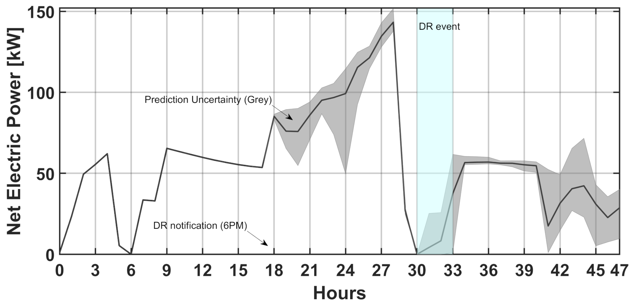
• Accounting for model prediction uncertainty due to weather forecast and identified model parameters was done by evaluating various uncertainty scenarios and by plotting the uncertainty bounds for the duration of the identified operation schedule.
• Contingency strategies were evaluated to quantify the energy flexibility available from the building to the grid at specific times. Two strategies were evaluated: (1) reducing the zone temperature setpoint for 3 h and (2) discharging the stored thermal energy in the ETS for 3 h.

3.1. Description of the Case Study Building and Electric Thermal Storage Device (ETS)

This study focuses on the energy flexibility potential of a building with an ETS storage system and using MPC as the control method. The controller’s objective is to minimize a cost function that may incorporate energy and/or power while maintaining the zone within reasonable comfort limits. This paper takes a step forward from Date et al. [39] to investigate MPC, the effects of uncertainties and predictions, and contingency reserve strategies.

This paper further evaluates more complex control strategies, namely MPC with different objective functions, and the potential for this building to help resolve contingency reserve issues of the electric grid. The objectives in this paper include minimization of cost under different scenarios on very cold days, improvements in operation during warmer shoulder season days, accounting for prediction uncertainties due to weather forecasts and model parameters, and participation in contingency events.

3.1.1. Description of the Case Study Building Zone

The investigated building zone is the warehouse portion of a two-storey office building located in Sherbrooke, Canada. The building was built in 1989 and has a floor area of 9000 m${}^2$, and the warehouse has a floor area of 1650 m${}^2$. The HVAC system servicing the warehouse section is equipped with an air-based ETS device with a rated maximum charging input of 106 kW. Data collection was ongoing since 2014 at 15-minute intervals for several measurements points. The peak load of the building was measured in February 2015 at 600 kW, with a monthly consumption of 166 MWh. The on-site 106 kW ETS supplies hot air to a warehouse zone in the building.

Figure 2 depicts how heat is delivered to the warehouse zone by the HVAC system [39]. Sensors measuring air temperatures are located throughout the HVAC system, and four thermocouples are embedded in the ETS, which measure brick temperatures. During operation of the ETS, a portion of supply air is directed to the thermal storage device to provide the zone with increased heat from stored heat energy. The zone is modeled using a 1R1C explicit finite difference modeling approach (Figure 3), with a heating coil model with proportional-integral control. The zone model was originally developed for a previous study [39] and was calibrated using several days of measured data from the real building. Statistical indices were found for a Root-Mean-Square Error (RMSE) of 0.75 ${}^{\circ }$C and a Mean Absolute Error (MAE) of 0.66 ${}^{\circ }$C. This simple model was used for demonstration of the overall methodology presented in this study and was sufficient for shorter control horizons, such as the ones evaluated here (1 or 2 days). C is the equivalent thermal capacitance of the zone, $T_{air}$ is the effective operative temperature of the zone, R is the equivalent resistance of the zone, and $q_{aux}$ is all heating sources to the zone air node. Solar gains had little influence on the behaviour of the warehouse zone, especially during the winter season. It is acknowledged that the building model is extremely simple; however, this does not make the proposed methodology less meaningful.

The system control variables are shown in Figure 4. The control variables are as follows:

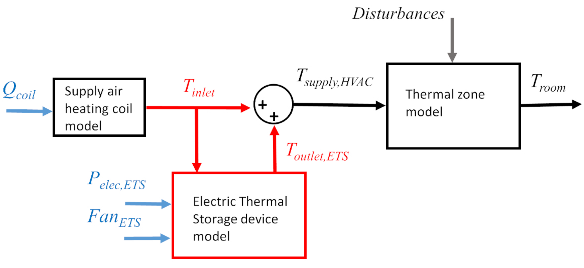
• ${\mathit{P}}_{\mathit{elec},\mathit{ETS}}$: the electric power to the ETS providing heat to the brick storage medium,
• ${\mathit{Fan}}_{\mathit{ETS}}$: the fan operation (ON/OFF), which notifies when air is passed through the brick storage medium,
• ${\mathit{Q}}_{\mathit{aux}}$: the additional auxiliary heating supplied to the supply air.

$T_{inlet}$ is the air temperature entering and bypassing the ETS; $T_{outlet,ETS}$ is the ETS outlet air temperature; and $T_{supply,HVAC}$ is the zone supply air temperature. $T_{room}$ is the air temperature of the warehouse zone.

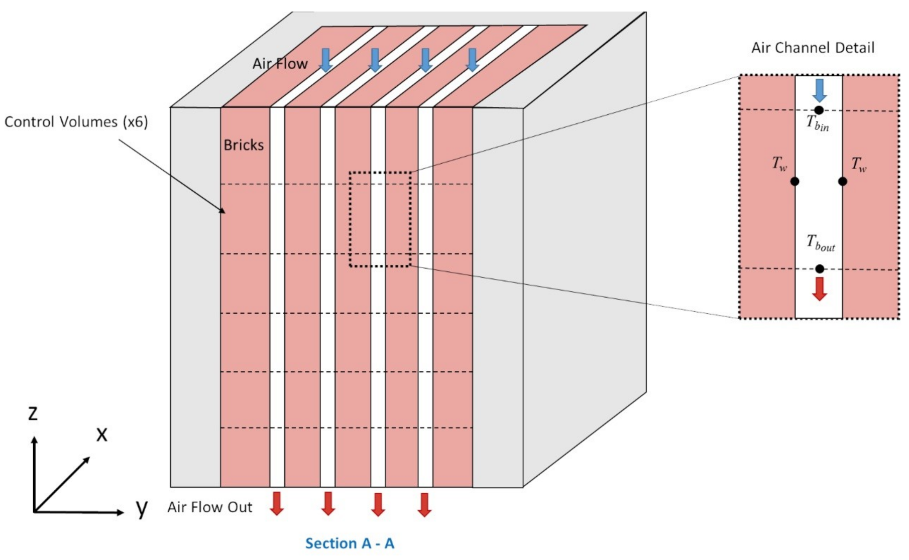
3.1.2. Description of Thermal Energy Storage Device

During times of reduced electricity prices or when demand is low on the grid, ETS systems store heat converted from electrical power. They provide heat from stored energy to the building during times of higher demand or high electric pricing [40]. They can deliver a noteworthy reduction in electricity bills when there is dynamic TOU tariffs or when the utility pricing structure has a demand charge [41,42]. They use specially designed bricks as a storage medium, and they release heat to circulating air or water and deliver it to the building zone. The device considered here contains 3121 kg of magnesite bricks in an insulated heat storage tank. Heating elements made from electric wires are located between the rows of bricks. The bricks are rated for a maximum temperature of 871 ${}^{\circ }$C. The total storage capacity is 640 kWh (2184 kBTU). A fan is used to send air to the device to recover heat. Specifications for the ETS are shown in

Table 1. Electric Thermal Storage (ETS) device specifications [39].

Parameter	Value
Electric Charging Input	106 kW
Thermal Storage Capacity	640 kWh
Storage Material	High-density ceramic bricks
Number of Heating Elements	24
Maximum Brick Temperature	871 ${}^{\circ }$C
Weight of Bricks	3121 kg
Number of Bricks	384

, and the schematics are shown in Figure 5 and Figure 6 [39].

Control of the device is based on several factors: (1) determining when to charge the storage medium, (2) control of the maximum temperature during the charging, and (3) control of total amount of stored heat. During the discharge cycle, a consistent outlet air temperature is internally controlled by the device.

The maximum brick temperature setting is based on a function related to the outdoor ambient temperature (depicted in Figure 7) and available power of the building. Once per day, a reading of the outdoor air temperature is used to set the maximum brick temperature.

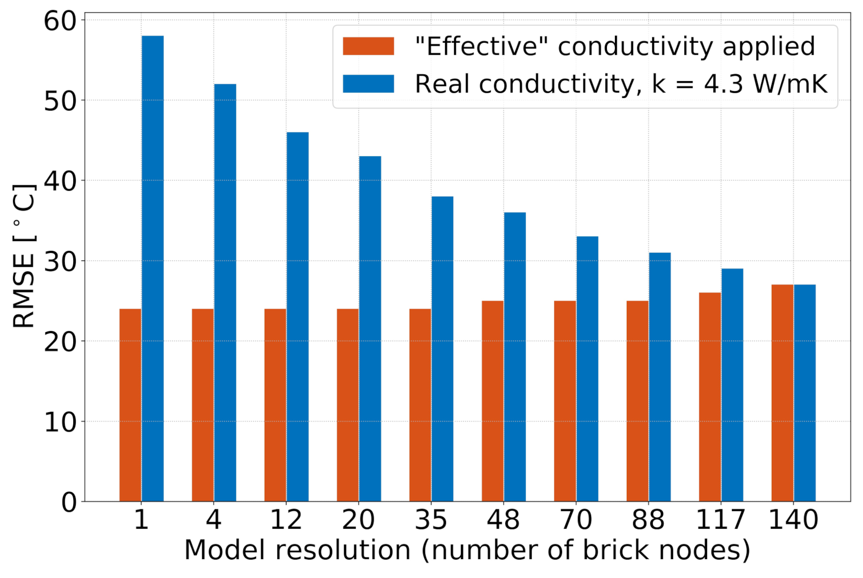
3.2. Control-Oriented Thermal Model

The control-oriented models are described below (first introduced in a precursor study [39]). The models were derived from energy conservation and heat conduction equations in the two-dimensional lumped parameter formulation. A grey-box modeling approach was employed, where physically meaningful parameters can be calibrated and/or identified using information of the building construction and measurement data.

The simulation code of the models were developed using MATLAB and can be conveniently modified to adjust the model order. The model order was automatically adjusted from very simple (1 node) to more detailed by defining the two-dimensional grid of rows and columns of brick nodes. The number of rows multiplied by the number of columns was thus the total number of brick capacitance nodes for that given model order. Easy and quick modifications of the model are thus possible without rewriting the simulation code.

Figure 5 depicts the 1-capacitance model as an example, and further details on the modeling methodology can be found in [39]. The network was comprised of one row along the x-axis, one column along the y-axis, and the convective conductance term connected with the zone air node.

The bricks were heated up by the electric wires, and thermal energy was transferred to the bricks. The lumped parameter finite difference method used in this study was based on the material discretized into control volumes, where a node is located at the centroid of the control volume (Equation (1)).

$$T_i^{p+1}=T_i^p+\frac{\Delta t}{C_i}\left[Q_i^p+\sum _{j=1}^n\frac{T_j^p-T_i^p}{R_{i,j}}\right]$$

(1)

where the node temperature is T, $R_{i,j}$ is the thermal resistance between nodes, $Q_i$ is the heat generated/received at a node, and C is the thermal capacitance ($C=\rho c_{p}Adx$). n is the number of nodes connected to i. Figure 5 shows the first-order model, and the brick temperature is calculated in Equation (2). The 1R1C zone model in Figure 3 was also solved using an equation similar to (1).

$$\begin{array}{c}\hfill T_{bricks}^{p+1}=T_{bricks}^p+\frac{\Delta t}{C_{bricks}}\left[Q_{source}^p-Q_{conv}^p+4·\frac{1}{R_{bricks}}\left(T_{ins}^p-T_{bricks}^p\right)+\frac{1}{R_{inf}}\left(T_{room}^p-T_{bricks}^p\right)\right]\end{array}$$

(2)

where $T_{bricks}$ is the temperature of all the bricks, $C_{bricks}$ is the thermal capacitance for all bricks, $Q_{source}$ is the heating power input, $Q_{conv}$ is the heat transferred from the bricks to the air in the air channel, $R_{bricks}$ represents $1/4$ of total brick resistance, $T_{ins}$ is the insulation layer surface temperature, $R_{inf}$ is the infiltration to the mechanical room, and $T_{room}$ is the mechanical room air temperature. In a previous paper investigating model complexity, it was found that adequate predictions were achieved using a slightly modified simple model. The reader is referred to Appendix B and the study by Date et al. [39] for further details on the ETS model.

3.3. Quebec Commercial Customer Electricity Rates

In the province of Quebec, Canada, there are utility rates that depend on the energy consumption and peak power demand of a building (or group of buildings) owned by the customer. Rate M, which is for the large commercial building sector, has a demand charge and two energy prices [43], as outlined in

Table 2. Pricing structure of utility rate M and rate flex M.

Rate M Large Commercial Building Sector
Demand Charge	$14.58/kW
First 210,000 kWh energy consumed	5.03¢/kW
Remaining energy consumbed	3.73¢/kW
Rate Flex M Large Commercial Building Sector
Winter 1 Dec.–31 Mar.
Demand Charge	$14.58/kW
Price of energy consumed outside peak events	3.17¢/kW
Price of energy consumed during peak events	50.00¢/kW
Summer 1 Apr.–30 Nov.
Demand Charge	$14.58/kW
First 210,000 kWh energy consumed	5.03¢/kW
Remaining energy consumbed	3.73¢/kW

. A unique feature of this rate is that, at any given month, the minimum demand charge applied is set to 65% of the peak winter load. This means that appropriate attention should be given to the operation strategies over the winter period where peak demand is highest due to large space heating loads.

3.4. Predictive Load Management Scenarios

Currently, control of the maximum power charging input to the ETS is determined based on a linear scale function relating outdoor temperature to the power input, as shown in

Table 3. Control of ETS power input: scale function.

${\mathit{T}}_{\mathit{ext}}$	${\mathit{P}}_{\mathit{ETS}}$	Brick Temperature
0 ${}^{\circ }$C	0%	93 ${}^{\circ }$C
−18 ${}^{\circ }$C	100%	871 ${}^{\circ }$C

and Figure 7.

By incorporating predictions of occupancy schedules and weather over the next day or two into the control sequence, optimal values of the maximum ETS charging input at each hour are identified that minimize electricity costs while maintaining the desired space conditioning of the warehouse zone. Simultaneously, the zone temperature profile is identified, which minimizes the following cost functions.

Three cost functions incorporating the two aforementioned utility rate structures and $BEFI$ were implemented, and their results were compared to the typical manual control currently in operation.

1.

Cost function using rate M: formulation of the first optimization problem is shown in Equation (3). The utility rate M in Table 2 is used as the cost function.

$$\begin{array}{cc}\hfill \underset{T_{SP},P_{ETS,maxSP}}{min}& J_{PH}=\left(\sum _{i=1}^N{P}_i\Delta t\right)·\left({\mathrm{Cos}\mathrm{t}}_{\mathrm{Energy}}\right)+\max \left(\mathit{P}\right)·\left({\mathrm{Cos}\mathrm{t}}_{\mathrm{Demand}}\right)\hfill \\ \hfill \mathrm{subject}\mathrm{to}& T_{SP,min}\le T_{SP}\le T_{SP,max}\hfill \\ \hfill & 0\le P\le P_{max}\hfill \\ \hfill & 0\le P_{ETS,maxSP}\le P_{ETS,max}\hfill \end{array}$$

(3)

2.

Cost function using rate flex M: the second optimization problem in consideration is shown in Equation (4), where the objective is the minimization of the variable electricity cost shown in Figure 8. Equation (4) is a special case of Equation (3) but has an added variable energy cost over the day, indicated by subindex i, with higher cost during peak hours (Table 2).

$$\begin{array}{cc}\hfill \underset{T_{SP},P_{ETS,maxSP}}{min}& J_{PH}=\left(\sum _{i=1}^N{P}_i\Delta t\right)·\left({\mathrm{Cos}\mathrm{t}}_{\mathrm{Energy},i}\right)+\max \left(\mathit{P}\right)·\left({\mathrm{Cos}\mathrm{t}}_{\mathrm{Demand}}\right)\hfill \\ \hfill \mathrm{subject}\mathrm{to}& T_{SP,min}\le T_{SP}\le T_{SP,max}\hfill \\ \hfill & 0\le P\le P_{max}\hfill \\ \hfill & 0\le P_{ETS,maxSP}\le P_{ETS,max}\hfill \end{array}$$

(4)

where N is the number of time steps over the prediction horizon $PH$ (24, 36, 48 h, etc.), $P_i$ is the power demand at time i, and $\Delta t$ is the time step. The objective is to identify two variables that minimize the cost associated with the utility rate charge: (1) an optimized setpoint schedule for the room temperature $T_{SP}$ and (2) the maximum charging power input to the ETS, $P_{ETS,maxSP}$. The setpoint is constrained by a lower ($T_{SP,min}$) and upper ($T_{SP,max}$) bound to maintain a level of thermal comfort for the zone occupants. The demand due to space heating P is constrained by the size of the heating equipment $P_{max}$. Similarly, the maximum charging power input to the ETS is constrained by the specifications of the device, $P_{ETS,max}$. Prediction control simulations are run at 5-minute intervals for higher time granularity and optimized values are identified at 1-hour intervals to speed up schedule identification.

3.

Cost function using BEFI maximization during peak demand: the last optimization problem considered is using BEFI as the cost function. A BEFI is maximized during a specified period of the peak demand event.

$$\begin{array}{cc}\hfill \underset{T_{SP},P_{ETS,maxSP}}{max}& J_{PH}=\mathrm{avg}{[P_{ref}-P_{flex}]}_{,\mathit{during}\mathit{DR}\mathit{event}}\hfill \\ \hfill \mathrm{subject}\mathrm{to}& T_{SP,min}\le T_{SP}\le T_{SP,max}\hfill \\ \hfill & 0\le P\le P_{max}\hfill \\ \hfill & 0\le P_{ETS,maxSP}\le P_{ETS,max}\hfill \end{array}$$

(5)

Equation (6) shows a more formal representation of the BEFI [3].

$$\begin{array}{ccc}\hfill & BEFI\left(t,\Delta t,t_{notice}\right)=\hfill & \hfill \frac{{\int }_t^{t+\Delta t}{P}_{ref}dt-{\int }_t^{t+\Delta t}{P}_{flex}dt}{\Delta t}\end{array}$$

(6)

where $BEFI$ is the Building Energy Flexibility Index, t is the start time of event, $\Delta t$ is the duration of event, $t_{notice}$ is time of notification for the event, $P_{ref}$ (kW) is the power demand from the reference scenario during an event, and $P_{flex}$ (kW) is the power demand from a flexibility case during an event. The $BEFI$ is the average difference between the power demand of the reference case, $P_{ref}$ (kW), and the power demand of the alternative “flexibility scenario”, $P_{flex}$ (kW), for the given event duration $\Delta t$, shown in equation 6. $BEFI$ could also be represented as a percentage by dividing it by the value of $P_{ref}$.

3.5. Real-Time Optimizing Algorithm

The MATLAB function fmincon uses a sequential quadratic programming algorithm and a line search method to find the minimum of a constrained nonlinear multi-variable function. The optimization algorithm in this paper identifies an hourly zone temperature setpoint schedule and maximum power input to the ETS.

3.6. Prediction and Control Horizons

Typically, in MPC, the optimal control problem is solved at each defined control step by looking ahead at forecast weather and occupancy schedules over the prediction horizon, $PH$. The prediction horizon is a time period where we have reasonably reliable information, ranging from a few hours to a couple of days. Using data available from the prediction horizon period, an optimization routine is solved and an optimal sequence of control moves is identified through the implementation of MPC. The identified schedules and control moves are applied to the building over a “control horizon”, which can be the same length or be shorter than the prediction horizon. Once the current control horizon has ended, the optimization exercise is performed again for the following prediction horizon. This process is repeated until the end of the simulation time (e.g., one day or one year). For the sake of simplicity, in this particular case, the prediction and control horizon are the same length of time and MPC was only initiated with a notification signal: either 30 h for a 12-hour ahead notification at 6 p.m. or 22 h for a 4-hour ahead notification at 2 a.m. (for a DR event at 6 a.m.). Further studies could be carried out on performance related to the control horizon length; however, Date et al. [44] found that longer control horizons (12 h or more) were favourable for a similar building in a similar climate.

4. Results and Discussion

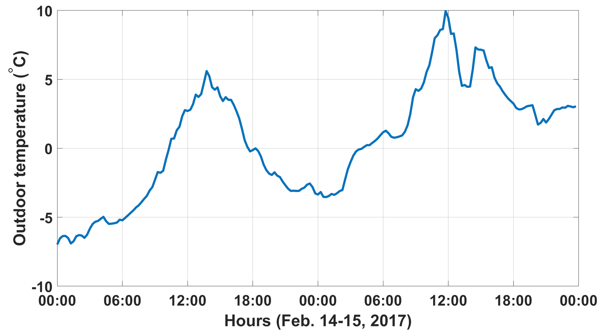
4.1. Weather Conditions—Cold Winter Day

MPC simulations were carried out over 10 days, with a focus on the last 48-hour period, with outdoor temperature conditions ranging from −20 ${}^{\circ }$C to 3 ${}^{\circ }$C (Figure 9). A business as usual (BAU) indoor temperature setpoint profile, with a nighttime setpoint of 18 ${}^{\circ }$C and a daytime setpoint of 22 ${}^{\circ }$C, was created as a benchmark, which is shown in the top graph of Figure 10 as a dashed black line. For the MPC studies, the zone temperature setpoint was constrained by a lower bound $T_{SP,min}$ (17 ${}^{\circ }$C at night and 19 ${}^{\circ }$C during the day) and an upper bound $T_{SP,max}$ (24 ${}^{\circ }$C at all times) in order to maintain a level of thermal comfort for the zone occupants. To demonstrate the methodology, typical known occupancy schedules for the warehouse (7 a.m.–6 p.m.) and weather data were used for this MPC study; however, an existing weather forecast tool such as CanMETEO [45] could be incorporated into eventual implementation within the building automation system in a real building.

4.2. Demand Response with 12- and 4-Hour Notifications

A scenario with a notification of demand response event given 12 h prior was investigated. The notification is given to the building owner at 6 p.m., indicating a DR event the following day at 6 a.m. and ending at 9 a.m. (3 h duration). The notification triggers an MPC algorithm that determines (a) an optimized zone temperature setpoint profile and (b) an optimized maximum allowable power input for charging the ETS device at each timestep. A second approach is conducted with a notification of 4 h ahead of the DR event at 2 a.m.

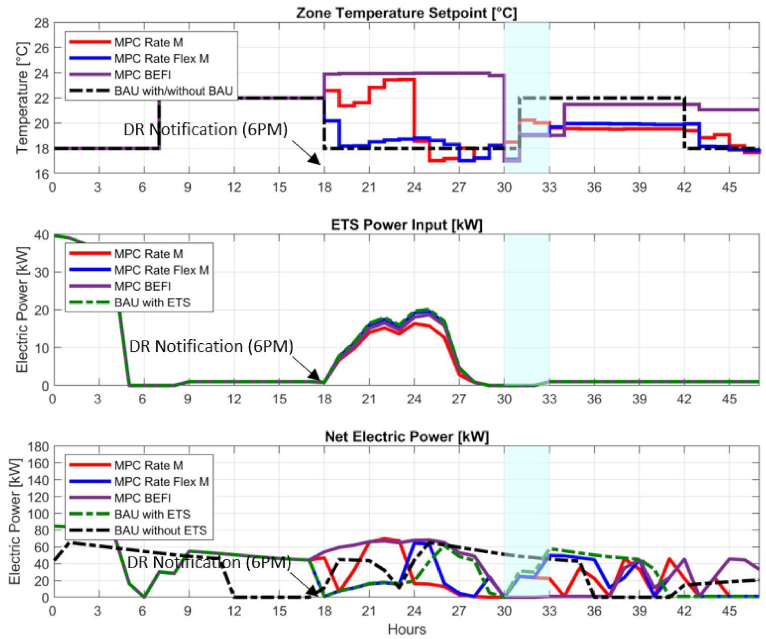
4.3. Predictive Load Management Simulation

Table 4. Model Predictive Control (MPC) simulation results for improved operation of ETS and zone temperature setpoint on a very cold day.

	BAU without Thermal Storage	BAU with Thermal Storage	MPC: Rate M	MPC: Rate Flex M	MPC: BEFI
12 h ahead notification of DR event (18:00)
Event Peak (kW) (6 a.m.–9 a.m.)	73	33	31	0	0
Wh/m${}^2$ in $PH$	763	1170	905	1034	1321
BEFI (kW) (6 a.m.–9 a.m.)	–	36	36	65	65
BEFI (%) (6 a.m.–9 a.m.)	–	55	56	100	100
4 h ahead notification of DR event (2:00)
Event Peak (kW) (6 a.m.–9 a.m.)	73	33	28	25	0
Wh/m${}^2$ in $PH$	659	844	641	633	945
BEFI (kW) (6 a.m.–9 a.m.)	–	36	38	48	65
BEFI (%) (6 a.m.–9 a.m.)	–	55	59	74	100

show the simulation results for the different scenarios. The scenarios (1) BAU with ETS, (2) MPC rate M, (3) MPC rate flex M, and (4) MPC BEFI are compared to the “Business as Usual (BAU)” case without ETS.

Figure 10 shows the MPC results for the case when a notification is given 12 h before a DR event, while Figure 11 shows the results for the case with 4 h notification time. Implementing MPC with active thermal storage can increase the value of BEFI and give energy flexibility to the grid during critical peak events; operation is also improved compared to BAU with ETS. As shown in Table 4, with a notification from the utility to the customer given at 6 p.m. (12 h ahead of an event at 6 a.m.) a BEFI of 55% to 100% is achieved. In other words, the peak demand during the critical event hours can be reduced by an average of 36 kW (63%) up to 65 kW (8%) for 3 h, depending on the utility rate structure. There were two identified scenarios where zero power demand for heating was required during the critical morning hours of 6 a.m. to 9 a.m., giving a BEFI of 100%.

It was found that rate flex M is the most successful in reducing the peak demand, while a greater reduction in energy consumption on a 24-hour period is seen with rate M. A longer notification time also results in a higher BEFI during the critical times, as there is more time for the MPC to identify improved operation strategies or implement preheating. When the equation for BEFI is used as the objective function, favourable results for peak reduction are found and are comparable with the scenario of the rate flex M; however, one disadvantage is that there is no incentive to reduce energy, and this results in this scenario with a high energy consumption (13% more compared to BAU with thermal storage at 1321 Wh/m${}^2$).

Similarly, with a relatively short notification time of 4 h (given at 2 a.m.), MPC can help reduce the peak demand during the critical hours and can achieve a BEFI of up to 48 kW (74%) for 3 h with rate flex M (Table 4). The results show that implementing MPC with active thermal storage and a properly chosen objective function can increase BEFI and give energy flexibility to the grid during critical peak events.

4.4. Shoulder Season Performance: Cold Day Followed by a Warm Day

Building energy performance during the shoulder seasons is also critical as it is easy to consume unnecessary energy on warmer days with an improper control strategy. The current practice for control strategies of the thermal storage device often use unnecessary energy by charging the bricks and by storing too much thermal energy when a warmer day is on the horizon. Typically, the ETS will look at the weather one time at 6 p.m. to determine the charging needed during the night for use of the stored energy the next day. Sometimes, when a cold day is followed by a warm day, this determined charging amount would be unnecessary and excess electricity would be used to store thermal energy when the needed thermal energy the next day is actually much less. Incorporating weather forecasts into the decision-making process for determining the charging input amount could improve energy use. An example of a cold day followed by a warm day is shown in Figure 12, where at 6 p.m., the outdoor temperature is below 0 ${}^{\circ }$C, but the next day is warmer, going as high as 10 ${}^{\circ }$C.

The results shown in Figure 13 and

Table 5. MPC simulation results for improved operation of ETS and zone temperature setpoint on a warmer shoulder season day.

	BAU without Thermal Storage	BAU with Thermal Storage	MPC: Rate M	MPC: Rate Flex M	MPC: BEFI
12 h ahead notification of DR event (18:00)
Event Peak (kW) (6 a.m.–9 a.m.)	65	31	25	25	0
Wh/m${}^2$ in $PH$	490	454	389	386	614
BEFI (kW) (6 a.m.–9 a.m.)	–	25	41	41	57
BEFI (%) (6 a.m.–9 a.m.)	–	55	68	75	100
4 h ahead notification of DR event (2:00)
Event Peak (kW) (6 a.m.–9 a.m.)	65	31	26	24	0
Wh/m${}^2$ in $PH$	456	443	259	328	395
BEFI (kW) (6 a.m.–9 a.m.)	–	25	41	41	57
BEFI (%) (6 a.m.–9 a.m)	–	55	71	72	100

correspond to shoulder season MPC simulation studies evaluating the performance using the three previously studied objective functions (rate M, rate flex M, and BEFI) with notifications at 12-hour and 4-hour ahead of an event. Even a warm shoulder season day can benefit from advanced MPC strategies, where energy consumption is lowered by up to 43% and a BEFI of up to 100% can be obtained. It is seen that both rate M and rate flex M give favourable results on a warm shoulder season day; however, an objective function of BEFI increases energy consumption and is not suitable for this type of day, where the more prevalent objective is to better manage (or reduce) energy use.

4.5. Accounting for Prediction Uncertainty

Presenting a range of reasonable operating predictions that take into account uncertainties related to weather forecasting and identified model parameter values can aid decision makers in assessing the risk in operation options available to them. Uncertainty in weather forecasts can be as high as 30%, and modeling uncertainty can be in that range as well.

Six scenarios of combinations incorporating $\pm 10\%$ deviation from the identified brick conductivity and ±3 ${}^{\circ }$C deviation from the weather forecast [39] were evaluated and are presented in this section. These six scenarios were carried out for the three different cost functions (rate M, rate flex M, and BEFI) at the two notification times (12 h and 4 h), for a total of 36 cases.

From the Figure 14, Figure 15 and Figure 16, one can make an informed decision about whether enabling a more advanced control strategy (in this case MPC) can be beneficial and whether the associated risk is appropriate. Figure 16 illustrates an example of how the net electric power prediction could vary depending on accuracy of the weather forecast and identified model parameter $k_{brick}$ when an identified operating schedule is obtained using an objective function of rate flex M. In other words, the grey area is a set of possible trajectories of the net power curve. Incorporating this type of evaluation and visualization in the decision-making process of building operators/owners and the utility grid would allow for a better understanding of the anticipated variations due to uncertainties in the problem. Future work could include incorporating an existing weather forecasting tool into the methodology, such as CanMETEO [45], to further evaluate the effects of weather uncertainty in MPC performance.

4.6. Contingency Event Evaluation

The contingency reserve is an amount of power that the utility may call when needed to face a loss of a generation unit or other unexpected load unbalances. To address this need, real-time thermal load flexibility must be predicted ahead of time or calculated continuously and available at short notice (e.g., 10 min) over a time duration of about an hour or a few hours.

This energy flexibility can be enabled by actions in response to a signal from the grid. This section calculates such a BEFI (kW and %) in order to quantify real-time thermal load flexibility of the building. A preliminary contingency study on a school building was introduced in [3]. Two strategies were analyzed: (1) reducing the zone temperature setpoint for a duration of 3 h and (2) discharging the thermal storage device for a duration of 3 h. An example of strategy (1) is depicted in Figure 17.

The available energy flexibility may be quantified using the developed model to determine the power demand difference between the reference case (BAU, no ETS) with the two contingency strategies outlined in the previous paragraph.

In strategy 1, shown in Figure 18 where the zone temperature setpoint is reduced by 2 ${}^{\circ }$C for 3 h, the BEFI varies from 0 up to 47 kW (or 0 up to 100%). The BEFI in this scenario is dependent on the time of day due to the reference case nighttime setback zone temperature schedule.

For the second strategy of discharging heat from the thermal storage device for durations of 3 h, the results are shown in Figure 19. A BEFI of 0 to 41 kW (or 0 to 100%) is achievable with this contingency strategy. Favourable results were found for both of these options, where a BEFI of up to 47 kW (97%) is achieved for a duration of 3 h. The highest BEFI values are seen towards the start of the day as that is the time of biggest potential to reduce peaks due to the existing abrupt setpoint change from night setback to day time comfort levels. In the evening, a zero value for BEFI is seen due to the setpoint change back to the lowered night time value. There is zero heating demand and thus cannot be lowered any further, and the zone air temperature is free floating until the lower night time value is reached.

5. Conclusions

This paper presented a methodology for the implementation of MPC strategies to a building equipped with a dedicated active thermal storage device in order to predict and maximize the building energy flexibility that the building could provide to the electric grid by evaluating the BEFI related to the different strategies. Three MPC cost functions were studied: (1) minimization of the electricity cost subject to a utility rate with peak demand charge (rate M), (2) minimization of the electricity cost subject to a utility rate with dynamic pricing (rate flex M), and (3) maximization of BEFI during a critical DR event.

Given a notification 4 or 12 h ahead of a DR event with a given duration, MPC was implemented at an hourly time step to identify an optimized zone temperature setpoint profile and an optimized dynamic maximum allowable power input for charging the thermal storage device. The results show that implementing MPC with thermal storage can increase BEFI, can provide energy flexibility to the grid during critical peak events, and is better than manual control. It is seen not only that optimizingthe zone profile is important but also that optimizing (limiting) the maximum allowable power to the thermal storage device aids in reducing both peak demand and energy consumption of the building.

It should be acknowledged that thermal comfort conditions for the different scenarios are different from that of the BAU case, which should be considered when choosing a strategy. Since the zone in this study is a warehouse, more flexibility in the comfort limits could be assumed when compared to an office or residential building.

Future work could include using this methodology to design optimal utility pricing structures rather than the design optimal control strategies. Though the scope of this study was limited by data availability, the developed methodology could be transposed to other similar convectively conditioned buildings and clusters of buildings for participation in community-scale energy aggregator events. A greater focus on occupancy modeling could eventually be incorporated into this methodology. There is still work to be done in terms of implementation of the methodology into real building building energy management systems.

References

1. Denholm, P.; O’Connell, M.; Brinkman, G.; Jorgenson, J. Overgeneration from Solar Energy in California. Field Guide Duck Chart 2015. [Google Scholar] [CrossRef] [Green Version]
2. IEA. IEA EBC Annex 67. 2020. Available online: http://www.annex67.org/ (accessed on 1 February 2021).
3. Athienitis, A.K.; Dumont, E.; Candanedo, J.A.; Morovat, N.; Lavigne, K.; Date, J. Development of a dynamic energy flexibility index for buildings and their interaction with smart grids. In Proceedings of the Aceee Summer Study 2020 Conference, Pacific Grove, CA, USA, 17–21 August 2020. [Google Scholar]
4. Date, J.A.; Candanedo, J.A.; Athienitis, A.K.; Lavigne, K. Energy flexible building: Predictive load management of passive and active energy storage under a Demand Response Program. In Proceedings of the eSIM 2020 Conference, Vancouver, BC, Canada (Postponed), 15–16 June 2020. [Google Scholar]
5. Hydro-Quebec. Annual Report. 2018. Available online: https://www.hydroquebec.com/about/financial-results/annual-report.html (accessed on 1 February 2021).
6. Hydro-Québec Distribution. État D’Avancement 2012 du Plan D’Approvisionnement 2011–2020. 2012. Available online: http://www.regie-energie.qc.ca/audiences/TermElecDistrPlansAppro_Suivis.html (accessed on 1 February 2021).
7. Qin, S.; Badgwell, T.A. A survey of industrial model predictive control technology. Control. Eng. Pract. 2003, 11, 733–764. [Google Scholar] [CrossRef]
8. Sturzenegger, D.; Gyalistras, D.; Morari, M.; Smith, R.S. Model Predictive Climate Control of a Swiss Office Building. Proc. Clima Rheva World Congr. 2016, 24, 1–12. [Google Scholar] [CrossRef]
9. De Coninck, R.; Helsen, L. Practical implementation and evaluation of model predictive control for an office building in Brussels. Energy Build. 2016, 111, 290–298. [Google Scholar] [CrossRef]
10. Prívara, S.; Široký, J.; Ferkl, L.; Cigler, J. Model predictive control of a building heating system: The first experience. Energy Build. 2011, 43, 564–572. [Google Scholar] [CrossRef]
11. Perera, D.W.U.; Winkler, D.; Skeie, N.O. Multi-floor building heating models in MATLAB and Modelica environments. Appl. Energy 2016, 171, 46–57. [Google Scholar] [CrossRef]
12. Jensen, S.Ø; Marszal-Pomianowska, A.; Lollini, R.; Pasut, W.; Knotzer, A.; Engelmann, P.; Stafford, A.; Reynders, G. IEA EBC Annex 67 Energy Flexible Buildings. Energy Build. 2017, 155, 25–34. [Google Scholar] [CrossRef] [Green Version]
13. Reynders, G.; Amaral Lopes, R.; Marszal-Pomianowska, A.; Aelenei, D.; Martins, J.; Saelens, D. Energy flexible buildings: An evaluation of definitions and quantification methodologies applied to thermal storage. Energy Build. 2018, 166, 372–390. [Google Scholar] [CrossRef]
14. Le Dréau, J.; Heiselberg, P. Energy flexibility of residential buildings using short term heat storage in the thermal mass. Energy 2016, 111, 991–1002. [Google Scholar] [CrossRef]
15. Hurtado, L.; Rhodes, J.; Nguyen, P.; Kamphuis, I.; Webber, M. Quantifying demand flexibility based on structural thermal storage and comfort management of non-residential buildings: A comparison between hot and cold climate zones. Appl. Energy 2017, 195, 1047–1054. [Google Scholar] [CrossRef]
16. Weiß, T.; Fulterer, A.M.; Knotzer, A. Energy flexibility of domestic thermal loads–a building typology approach of the residential building stock in Austria. Adv. Build. Energy Res. 2019, 13, 122–137. [Google Scholar] [CrossRef]
17. Vigna, I.; Pernetti, R.; Pasut, W.; Lollini, R. New domain for promoting energy efficiency: Energy Flexible Building Cluster. Sustain. Cities Soc. 2018, 38, 526–533. [Google Scholar] [CrossRef]
18. Foteinaki, K.; Li, R.; Heller, A.; Rode, C. Heating system energy flexibility of low-energy residential buildings. Energy Build. 2018, 180, 95–108. [Google Scholar] [CrossRef]
19. Junker, R.G.; Lindberg, K.B.; Reynders, G.; Lopes, R.A.; Relan, R.; Azar, A.G.; Madsen, H. Characterizing the energy flexibility of buildings and districts. Appl. Energy 2018, 225, 175–182. [Google Scholar] [CrossRef]
20. Liu, M.; Heiselberg, P. Energy flexibility of a nearly zero-energy building with weather predictive control on a convective building energy system and evaluated with different metrics. Appl. Energy 2019, 233–234, 764–775. [Google Scholar] [CrossRef]
21. Reynders, G.; Diriken, J.; Saelens, D. Generic characterization method for energy flexibility: Applied to structural thermal storage in residential buildings. Appl. Energy 2017, 198, 192–202. [Google Scholar] [CrossRef] [Green Version]
22. Aduda, K.O.; Labeodan, T.; Zeiler, W.; Boxem, G.; Zhao, Y. Demand side flexibility: Potentials and building performance implications. Sustain. Cities Soc. 2016, 22, 146–163. [Google Scholar] [CrossRef]
23. Sánchez Ramos, J.; Pavón Moreno, M.; Guerrero Delgado, M.; Álvarez Domínguez, S.F.; Cabeza, L. Potential of energy flexible buildings: Evaluation of DSM strategies using building thermal mass. Energy Build. 2019, 203, 109442. [Google Scholar] [CrossRef]
24. Perez, K.X.; Baldea, M.; Edgar, T.F. ntegrated HVAC management and optimal scheduling of smart appliances for community peak load reduction. Energy Build. 2016, 123, 34–40. [Google Scholar] [CrossRef] [Green Version]
25. Sharma, I.; Dong, J.; Malikopoulos, A.A.; Street, M.; Ostrowski, J.; Kuruganti, T.; Jackson, R. A modeling framework for optimal energy management of a residential building. Energy Build. 2016, 130, 55–63. [Google Scholar] [CrossRef]
26. Patteeuw, D.; Henze, G.P.; Helsen, L. Comparison of load shifting incentives for low-energy buildings with heat pumps to attain grid flexibility benefits. Appl. Energy 2016, 167, 80–92. [Google Scholar] [CrossRef]
27. Cigler, J.; Tomáško, P.; Široký, J. BuildingLAB: A tool to analyze performance of model predictive controllers for buildings. Energy Build. 2013, 57, 34–41. [Google Scholar] [CrossRef]
28. Donghun, K.; Braun, J.E. Reduced-order building modeling for application to model-based predictive control. In Proceedings of the Fifth National Conference of IBPSA-USA, Madison, WI, USA, 1–3 August 2012. [Google Scholar]
29. Kummert, M.; André, P.; Nicolas, J. Optimal heating control in a passive solar commercial building. Sol. Energy 2001, 69, 103–116. [Google Scholar] [CrossRef]
30. Oldewurtel, F.; Parisio, A.; Jones, C.N.; Gyalistras, D.; Gwerder, M.; Stauch, V.; Lehmann, B.; Morari, M. Use of model predictive control and weather forecasts for energy efficient building climate control. Energy Build. 2012, 45, 15–27. [Google Scholar] [CrossRef] [Green Version]
31. Drgona, J.; Arroyo, J.; Cupeiro, I.; Blum, D.; Arendt, K.; Kim, D.; Oll, E.P.; Oravec, J.; Wetter, M.; Vrabie, D.L.; et al. All you need to know about model predictive control for buildings. Annu. Rev. Control. 2020. [Google Scholar] [CrossRef]
32. Prívara, S.; Vána, Z.; Záceková, E.; Cigler, J. Building modeling: Selection of the most appropriate model for predictive control. Energy Build. 2012, 55, 341–350. [Google Scholar] [CrossRef]
33. Touretzky, C.R.; Baldea, M. Nonlinear model reduction and model predictive control of residential buildings with energy recovery. J. Process. Control 2014, 24, 723–739. [Google Scholar] [CrossRef]
34. Moroşan, P.D.; Bourdais, R.; Dumur, D.; Buisson, J. Building temperature regulation using a distributed model predictive control. Energy Build. 2010, 42, 1445–1452. [Google Scholar] [CrossRef]
35. Hou, X.; Xiao, Y.; Cai, J.; Braun, J.E. A Distributed Model Predictive Control Approach for Optimal Coordination of Multiple Thermal Zones in a Large Open Space. In Proceedings of the Fourth International High Performance Building Conference at Purdue, West Lafayette, IN, USA, 11–14 July 2016. [Google Scholar]
36. Huang, H.; Chen, L.; Hu, E. Reducing energy consumption for buildings under system uncertainty through robust MPC with adaptive bound estimator. Proceedings of Fourth International High Performance Building Conference at Purdue, West Lafayette, IN, USA, 11–14 July 2016. [Google Scholar]
37. Jorissen, F.; Helsen, L. Towards an Automated ToolChain for MPC in Multi-zone Buildings. In Proceedings of the Fourth International High Performance Building Conference at Purdue, West Lafayette, IN, USA, 11–14 July 2016. [Google Scholar]
38. Date, J.A.; Candanedo, J.A.; Athienitis, A.K.; Lavigne, K. Control-Oriented Modeling of an Air-Based Electric Thermal Energy Storage Device. Proceedings of ASHRAE Winter Conference 2018, Chicago, IL, USA, 20–24 January 2018. [Google Scholar]
39. Date, J.A.; Candanedo, J.A.; Athienitis, A.K.; Lavigne, K. Development of reduced order thermal dynamic models for building load flexibility of an electrically-heated high temperature thermal storage device. Sci. Technol. Built Environ. 2020, 26, 956–974. [Google Scholar] [CrossRef]
40. Moffet, M.A.; Sirois, F.; Joos, G.; Moreau, A. Central electric thermal storage (ETS) heating systems: Impact on customer and distribution system. In Proceedings of the IEEE Power Engineering Society Transmission and Distribution Conference, Orlando, FL, USA, 7–10 May 2012. [Google Scholar] [CrossRef]
41. Bedouani, B.Y.; Labrecque, B.; Parent, M.; Legault, A. Central electric thermal storage (ETS) feasibility for residential applications: Part 2. Techno-economic study. Int. J. Energy Res. 2001, 25, 73–83. [Google Scholar] [CrossRef]
42. Syed, A.M. Electric Thermal Storage Option for Nova Scotia Power Customers: A Case Study of a Typical Electrically Heated Nova Scotia House. Energy Eng. 2011, 108, 69–79. [Google Scholar] [CrossRef]
43. Hydro-Québec. Hydro-Québec—Rates for Business Customers. 2020. Available online: http://www.hydroquebec.com/business/customer-space/rates/ (accessed on 1 February 2021).
44. Date, J.; Candanedo, J.; Athienitis, A.K. Predictive Setpoint Optimization of a Commercial Building Subject to a Winter Demand Penalty Affecting 12 Months of Utility Bills. In Proceedings of the Building Simulation 2017 Conference, San Francisco, CA, USA, 7–9 August 2017. [Google Scholar]
45. Natural Resources Canada. CanMETEO. 2019. Available online: https://www.nrcan.gc.ca/energy/canmeteo/19908 (accessed on 1 February 2021).
46. American Society of Heating Refrigerating and Air-Conditioning Engineers. Ashrae Handbook: Fundamentals; Ashrae: Atlanta, GA, USA, 2009. [Google Scholar]
Figure 1. Outline of the methodology.
Energies 14 01387 g001
Figure 2. Heating, Ventilation, and Air Conditioning (HVAC) system with Electric Thermal Storage (ETS) and temperature sensor locations [39].
Energies 14 01387 g002
Figure 3. Simple 1R1C thermal model of warehouse zone.
Energies 14 01387 g003
Figure 4. System schematic [39].
Energies 14 01387 g004
Figure 5. Top view of the ETS 1-capacitance thermal model [39].
Energies 14 01387 g005
Figure 6. Side view schematic of the brick discharging model [39].
Energies 14 01387 g006
Figure 7. Thermal storage power input depending on outdoor temperature.
Energies 14 01387 g007
Figure 8. Utility rate flex M over 24 h.
Energies 14 01387 g008
Figure 9. Outdoor air temperature on 12–13 February 2017: control study on cold days.
Energies 14 01387 g009
Figure 10. MPC utility rate study: identified zone setpoint profiles and electric power use with notification 12 h ahead for a cold winter day.
Energies 14 01387 g010
Figure 11. MPC utility rate study: identified zone setpoint profiles and electric power use with notification 4 h ahead for a cold winter day.
Energies 14 01387 g011
Figure 12. Control study on a cold day followed by a warm day: outdoor air temperature on 14 and 15 February 2017.
Energies 14 01387 g012
Figure 13. MPC utility rate study: identified zone setpoint profiles and electric power use with notification 12 h ahead for a warm shoulder season day.
Energies 14 01387 g013
Figure 14. Uncertainty of Building Energy Flexibility Index (BEFI) predictions: 12-hour ahead notification for a cold winter day.
Energies 14 01387 g014
Figure 15. Uncertainty of BEFI predictions: 4-hour ahead notification for a cold winter day.
Energies 14 01387 g015
Figure 16. Uncertainty of BEFI predictions: net electric power prediction for scenario with MPC rate flex M for a cold winter day.
Energies 14 01387 g016
Figure 17. Contingency strategy 1: reduce the zone temperature setpoint for a duration of 3 h at each hour—BEFI at hourly intervals
Energies 14 01387 g017
Figure 18. Contingency strategy 1: reduce the zone temperature setpoint for a duration of 3 h at each hour—BEFI at hourly intervals.
Energies 14 01387 g018
Figure 19. Contingency strategy 2: discharge the ETS for a duration of 3 h at each hour—BEFI at hourly intervals.
Energies 14 01387 g019